| Computers, Materials & Continua DOI:10.32604/cmc.2022.030392 | |
| Article |
Brain Tumor Detection and Classification Using PSO and Convolutional Neural Network
1Department of Computer Science, COMSATS University Islamabad, Wah Campus, Pakistan
2Departmnt of Computer Science, HITEC University Taxila, Pakistan
3Computer Sciences Department, College of Computer and Information Sciences, Princess Nourah Bint Abdulrahman University, Riyadh, 11671, Saudi Arabia
4College of Computer Engineering and Sciences, Prince Sattam bin Abdulaziz University, Al-Kharj, Saudi Arabia
5Department of EE, COMSATS University Islamabad, Wah Campus, Pakistan
6Department of Computer Science, Hanyang University, Seoul, 04763, Korea
7Center for Computational Social Science, Hanyang University, Seoul, 04763, Korea
*Corresponding Author: Byoungchol Chang. Email: bcchang@hanyang.ac.kr
Received: 25 March 2022; Accepted: 17 May 2022
Abstract: Tumor detection has been an active research topic in recent years due to the high mortality rate. Computer vision (CV) and image processing techniques have recently become popular for detecting tumors in MRI images. The automated detection process is simpler and takes less time than manual processing. In addition, the difference in the expanding shape of brain tumor tissues complicates and complicates tumor detection for clinicians. We proposed a new framework for tumor detection as well as tumor classification into relevant categories in this paper. For tumor segmentation, the proposed framework employs the Particle Swarm Optimization (PSO) algorithm, and for classification, the convolutional neural network (CNN) algorithm. Popular preprocessing techniques such as noise removal, image sharpening, and skull stripping are used at the start of the segmentation process. Then, PSO-based segmentation is applied. In the classification step, two pre-trained CNN models, alexnet and inception-V3, are used and trained using transfer learning. Using a serial approach, features are extracted from both trained models and fused features for final classification. For classification, a variety of machine learning classifiers are used. Average dice values on datasets BRATS-2018 and BRATS-2017 are 98.11 percent and 98.25 percent, respectively, whereas average jaccard values are 96.30 percent and 96.57% (Segmentation Results). The results were extended on the same datasets for classification and achieved 99.0% accuracy, sensitivity of 0.99, specificity of 0.99, and precision of 0.99. Finally, the proposed method is compared to state-of-the-art existing methods and outperforms them.
Keywords: Magnetic resonance imaging (MRI); tumor segmentation; deep learning; features extraction; classification
According to the American Cancer Society, approximately 12760 people died from brain tumors in 2005, out of a total of 18,500 cases reported. With the alarming death rate in mind, it is expected that by 2030, the number of cases will have increased to 26 million people, with 1.8 million people dying from brain cancer [1]. Magnetic resonance imaging (MRI) has so far played an important role in the medical field in segmenting brain tumors [2]. Segmentation is a process in which, images are subdivided into multiple parts or segments, and every single segment indicates some information like color, texture or intensity to detect image boundaries [3]. For tumor or infection segmentation, segmentation has played a critical role in the domain of medical image processing. The use of MRI-based brain tumor segmentation is an important step that includes tumor classification, functional imaging, and image registration. There are two types of brain tumors: primary tumors and secondary tumors [4]. The primary brain named as gliomas which start in the glial cell and begins within the brain cells. These are sometimes known as Oligodendroglia, meningiomas, schwannomas tumors. This type of tumor is classified as the non-malignant and it can spreads automatically [5]. In contrast, secondary tumor has the tendency to originate from the other part of the body and can spread towards the brain. During this travel it can create multiple numbers of brain tumor which is more lethal than its counterpart.
As far as the brain is concerned, it is the most significant organ of the human body and it has a very complex structure consisting of 50–100 billion neurons [6]. Brain tumor tissues are the cells that can affect the normal growth of the brain [7]. Since these tissues expands themselves within the brain to effect the brain cells. Generally, these are malignant in nature [8]. Recently, World Health Organization (WHO) categorized four different grades of glioma brain tumor. According to WHO first, two grades are low-grade gliomas (LGG), and the remaining two are high-grade gliomas (HGG) [9]. In HGG, after the tumor detection, the maximum survival time period is almost 14 months. The patient suffering with HGG Gliomas brain tumors can survive from 2 to 4 years. The survival percentage is 47.4% to 18.5% for 2 to 4 years respectively. Likewise the growth rate of LGG is slower the hence the survival rate is 57% up to 10 years [10].
Brain tumor is the growth of abnormal cells within the brain or near the brain, it can be classified as cancerous or non-cancerous [11]. Here it is pertinent to mention, that the brain is not just liable to suffer from diseases. Since it can also be damaged by the irregular growth of the cells that can change its natural shape and behavior [12]. Numerous types of cancers caused due to brain. These are kidney, lungs, breast cancer, and many more. Among all cancer types, the tumor is a common kind of cancer. Brain tumor is one of its types that is categorized into benign and malignant classes. The malignant type have cancerous cells, while the benign do not have cancerous cells [13]. In [14] the borders of the benign tumor are presented very clearly. The growth of benign tumor is very rapid but does not affect healthy cells. Therefore, it can remove easily using surgery or treatment because of Grade 1 and 2 natures. Common examples of benign tumor is Moles [15,16]. In contrast, the malignant tumors are dangerous with fast growth rate and effect other brain tissues as well. It can lead to cause death if it is not identified at the earliest stage. Almost approximately 80% Gliomas tumor cases are diagnosis as malignant [17].
There have been numerous methods introduced, including edge-based, thresholding, deformable models, and region-based segmentation methods. These methods are also extended to distinguish between benign and malignant tumors. These classification techniques are divided into two types: supervised and unsupervised methods. The supervised method reflects working of various classifiers including Support Vector Machine (SVM), Artificial Neural Network (ANN) and Bayes classifiers [18]. Similarly, but in an unsupervised classification/segmentation method are demonstrated using clustering algorithms including Fuzzy C Mean (FCM), thresholding based algorithm, edge based technique, K-Means, and atlas-based segmentation algorithm [19]. In [20], graph cut distribution is proposed and is used for 3D multimodal based brain glioma tumors segmentation. A simple tumor segmentation technique (SLIC) proposed in [21] consists of the clustering method. This technique employed mean and variance on BRATS 2015 dataset to resolve the image segmentation by taking maximum threshold value in order to improve and performance and accuracy. There are few brain tumor segmentation methods based on deep learning that incorporate MR images. The significant of MRI is that it presents various tumor characteristics in single image that include different sizes, shapes, and contrast. In [22], the proposed work used BRATS 2013 dataset is used to improve results using MRI. The proposed method has five steps. After image acquisition, the preprocessing method is applied to enhance the contrast of the images. Afterwards, Fuzzy C-mean method is applied to extract brain tumor followed by evaluation process. Finally, accuracy based results are demonstrated using ground truth images and different comparable methods.
The technique proposed in [23] is for automatic magnetic resonance (MR) brain tumor diagnostic system. The system contains of three basic stages to detect and segment a brain tumor. In the first stage, the preprocessing is adopted to remove noise from MRI images. Secondly, segmentation methods is proposed based on global thresholding approach. Finally, post-processing is adopted to reduce the false positives followed by morphological operation to determine the tumor part accurately in MR images. In [24], the proposed technique is based on a kernel fuzzy C-Means (KIFCM) brain tumor segmentation algorithm. In this work K-means clustering algorithm computes the tumor area efficiently. The algorithm reflects more precise segmentation results by introducing fuzzy C-Means (FCM) segmentation algorithm for MRI images. Since, the technique is suitable for removing noise from images. Therefore, they introduced method that used features to minimize the execution time and maximize segmentation results.
In [25], the proposed method is based on tumor region growth and separation. The important part of this technique, in which the increased tumor area is handled by image dilation. This approach helped to determine accurate ROI as an alternative of segmenting tumor area. Since tumor nearby tissues significantly presents various classes of brain tumor. Parallel to this, the augmented tumor area is gradually subdivided into finer ring-form subareas. Finally, the proposed system evaluates its competence on a large image dataset using various feature extraction methods such as intensity histogram, Gray Level Co-Occurrence Matrix (GLCM), and Bag-Of-Words (BoW) model. The experiment results show that the presented technique is effective for detecting brain tumors in T1-weighted contrast enhanced MRI. The method introduced in [26] for brain tumor segmentation is based on deep neural network (DNN). This method performs better for HGG and LGG grade MR images. This is all because of the reason that tumor has different size, color and shapes and can seem anywhere in the brain. The experiments are evaluated using BRATS 2013 dataset that is used for segmentation using novel deep neural network (DNN) model. Finally, the outcomes show that this methodology performs better among various competitive methods.
Detection and segmentation of the brain tumor is considered to be the challenging issue in the field of medical sciences [27]. There are many techniques developed for this purpose including k-means clustering, discrete cosine transform (DCT), Fuzzy C-Mean, and many more. Since, still there is a room available to improve the results in this regard. In this research work our main emphasis is early and accurate detection of the tumor found in distinct places. For this purpose, segmentation is applied in first step to segment the specific area of the brain where tumor found and after segmentation classification is done which correspond about which class the tumor belongs. Early detection methods are working without segmentation and their results are ambiguous that doesn’t conform to the efficient results.
In the proposed work, the Particle Swarm Optimization algorithm (PSO) is applied to segment brain tumor from MRI images. Afterwards, these segmented images are used for deep convolutional neural network (CNN) model using alexnet and inceptionV3. For doing this, we begin with the acquisition of MRI brain images. Firstly, the preprocessing of the MRI images is performed to obtain better results in latter stages. Secondly, the PSO algorithm is employed in order to segment tumor part, which is finally followed by post-processing to acquire accurate region of interest (ROI). The illustration of the proposed work is shown in Fig. 1. This figure depicts that three-steps have been employed in the preprocessing phase including image denoising, image sharpening, and skull stripping. These three-step ensures the enhancement MRI images for accurate segmentation and results. Likewise, in the segmentation phase, we are using the PSO algorithm for obtaining the best segmentation results to extract the tumor area of the brain MR Images. Finally, the post-processing step has been applied three-step have been followed which is image denoising, manually thresholding, and image binarization. This three-step make segmented images more enhance and give us maximum accuracy.

Figure 1: Proposed model of brain tumor segmentation and detection
Preprocessing is the most fundamental and difficult aspect of a computer-aided diagnostic system [28]. It is critical to preprocess the image for perfect tumor segmentation and feature extraction in the medical field so that the algorithm works properly. The tumor can be accurately segmented if the image is preprocessed according to its size and quality. Because of factors such as image acquisition, complex background, and low contrast, the preprocessing phase is very important in medical images. As a result, pre-processing is the major step on which the rest of the stages rely heavily. In the preprocessing phase, the three steps listed below were used. Image denoising, image sharpening, and skull stripping are examples of these. The process is adopted in the following manners:
Firstly, Gaussian Filter is used to remove noise from MRI Images. Fig. 2 reflect the results of this process that is denoising images using Gaussian filter. In the proposed work 2-D Gaussian smoothing filter is used to eliminate noise from the images, the purpose of this filter is to reduce the noise ratio. The general mathematical form of the 2-D Gaussian filter is given below:
In the above equation

Figure 2: BRATS-2018 and 2017 De-noisy images
Secondly, we have employed un-sharp masking for image enhancement. Finally, skull stripping technique is used to remove non-interested tissues, skull or boundaries present in the brain MR images.
2.2 Tumor Segmentation Using Particle Swarm Optimization
PSO algorithm is a population-based process motivated by the natural social behaviors, including birds flocking and fish schooling. PSO algorithm is very easy and energetic to achieve a conceivable solution. Due to this property the algorithm has applied to resolve an extensive variety of optimization problems. It was developed in 1995 by Kennedy and Eberhard [29]. This algorithm has now been applied in numerous types of optimization problems, such as robot control, Artificial Intelligence (AI) learning, image processing and many other fields of science. The particle swarm optimization algorithm is used to compute local best solution efficiently [30]. The benefit of the PSO algorithm has that it can improve accuracy and effectively used in many other fields [31]. Fig. 3 shows the results of the PSO segmentation algorithm. The input of the PSO algorithm for image segmentation are the following: Input: PSO(Cost-function, decision variables, L, U, and parameters) and Output: Segmented Image; Whereas the initial steps are as follows: Input image, Converted image into 3 channels, Set the number of clusters K = 4, Defined a cost function, Number of decision variables that are 12, Lower bound and upper bound, and Parameters such as maximum iterations that are 200. The detail algorithm description is given as follows:

Figure 3: Proposed PSO segmentation results
PSO Algorithm: Suppose O denotes the point of the particle and V denotes the velocity of the particle in the given search space. H denotes iteration where every particle x has its own position, the mathematical formulation of the velocity and particle is given below within the search space S.
For every next iteration, particle and velocity can be computed with the following formula.
In the PSO algorithm, the weight factor (
Post Processing: Following segmentation, post-processing is an important step. Several types of artifacts appear during the segmentation process. As a result, these artifacts can be removed in this step to obtain better results from segmented images. Three steps were taken during the post-processing phase: image denoising, manually thresholding, and image binarization. These three steps improve segmented images in order to achieve maximum accuracy during the classification phase. The procedure is as follows: i) After segmentation, a 2D-Median filter is used to remove noise and refine the images; ii) we used a manual thresholding method to detect ROI from the segmented images, which was then converted into binary form. The segmented image has only three grayscale levels, which can be arranged in descending order. In our work, we choose the top two and compute the mean of these two levels. As a result, this mean value serves as our threshold value, and iii) the Otsu binarization method is used to convert the grayscale image into binary form, from which we can extract the tumor area as needed.
In computer vision and machine learning deep CNN model are vigorously used for classification [33,34]. In deep CNN layers architecture, the image features can be targeted and process in following layer as shown in Fig. 4 [35]. Deep CNN models are commonly used nowadays due to their low computational cost. We used alexnet and the InceptionV3 model in the proposed work. To begin, we extract features from two pre-trained models, alexnet and inception-V3. These pre-trained models extract deep features from the data/images provided. After accomplishment features extraction process, then it is mandatory to resize the input images (240 × 240) into (256 × 256) for alexnet and inception-V3 and also convert RGB images Òmageimageinto grayscale using the following given formula.
where

Figure 4: Features extraction transferred learning model
In the above mathematical form Ò denote an images, q and w denote labels of training data of target and source domain. DCNN pre-trained model is used for training, and we get 1 × 4096 and 1 × 2048 features from alexNet and inception-v3 and using fully connected layer seven (FC7) and avg-pool layer respectively known as
Next step, after features extraction is to fuse features and get a final features vector. For this purpose, fully connected layers FC follow the same structure of feed forward network then it can be defined as:
where J represent input vector of
where
In this work, a novel method for brain tumor detection is proposed which is followed by classification using MRI images. The efficiency of the proposed method is tested on two datasets. Both of these datasets are publicly available that are named as BRATS-2017 and BRATS-2018 [36]. Both datasets contain a total of 285 MRI cases of the brain that are classified into HGG and LGG. HGG contains 210 MRI images of brain and LGG 75 brain images respectively and each class has 4 sequences of images including Flair (Fluid Attenuation Inversion Recovery), T1-weighted, T2-weighted, and T1ce. However, the tumor region is mostly highlighted in Flair and T2 images. The evaluation metrics including Dice, Jaccard Index, Jaccard distance, SSIM, F1 Score, precision, recall, error and time are computed while performing experiments. However, Jaccard Index basically compare two images in term of similarity as well as their differences If the percentage is higher than two images are seem to be identical Similarly Jaccard distance refers to how distinct two images are in term of their visibility and their shapes. Structural Similarity Index (SSIM) is basically the performance measures that determine how much quality of image degrade after the processing. The combination of precision and recall of classifier by taking their harmonic mean is considered as F1- Score Precision determines how much precisely the image conforms to the fact. Recall is the number of matched images by the sum of existing images. ERROR is something that wrongly predict/identifies the image. Classification results are also obtained from the proposed work. Figs. 5 and 6 illustrated the comparison of proposed segmentation work with ground truth images of both datasets respectively. Further, BRATS 2018 dataset is used to classify tumor images into HGG and LGG classes. For doing this, pre-trained alexnet and inception V3 model are used for classification with the help of Support Vector Machine (SVM). The pre-trained model of alexnet and inception V3 take image as input and perform different steps including convolution, polling, fully connected and finally SoftMax which produce classification results. In this classification process all SVM classification variants including Linear SVM, Quadratic SVM, Cubic SVM, Fine Gaussian SVM, Medium Gaussian SVM are utilized to check the efficacy of them on our proposed work. First all the data is trained with alexnet and inceptionv3 model then give it as input to classifiers. Several tests are performed, however few of them are mentioned in this section. Experimental results are taken using MATLAB 2019a on a core i7 system, having specifications 2.7 GHz Processor, 8.0 GB of RAM, and 64-bit Operating System (OS).

Figure 5: BRATS 2017 segmentation results of proposed work

Figure 6: BRATS 2018 segmentation results of proposed work
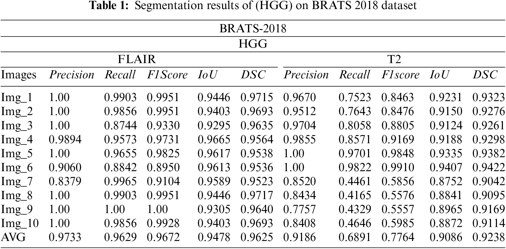
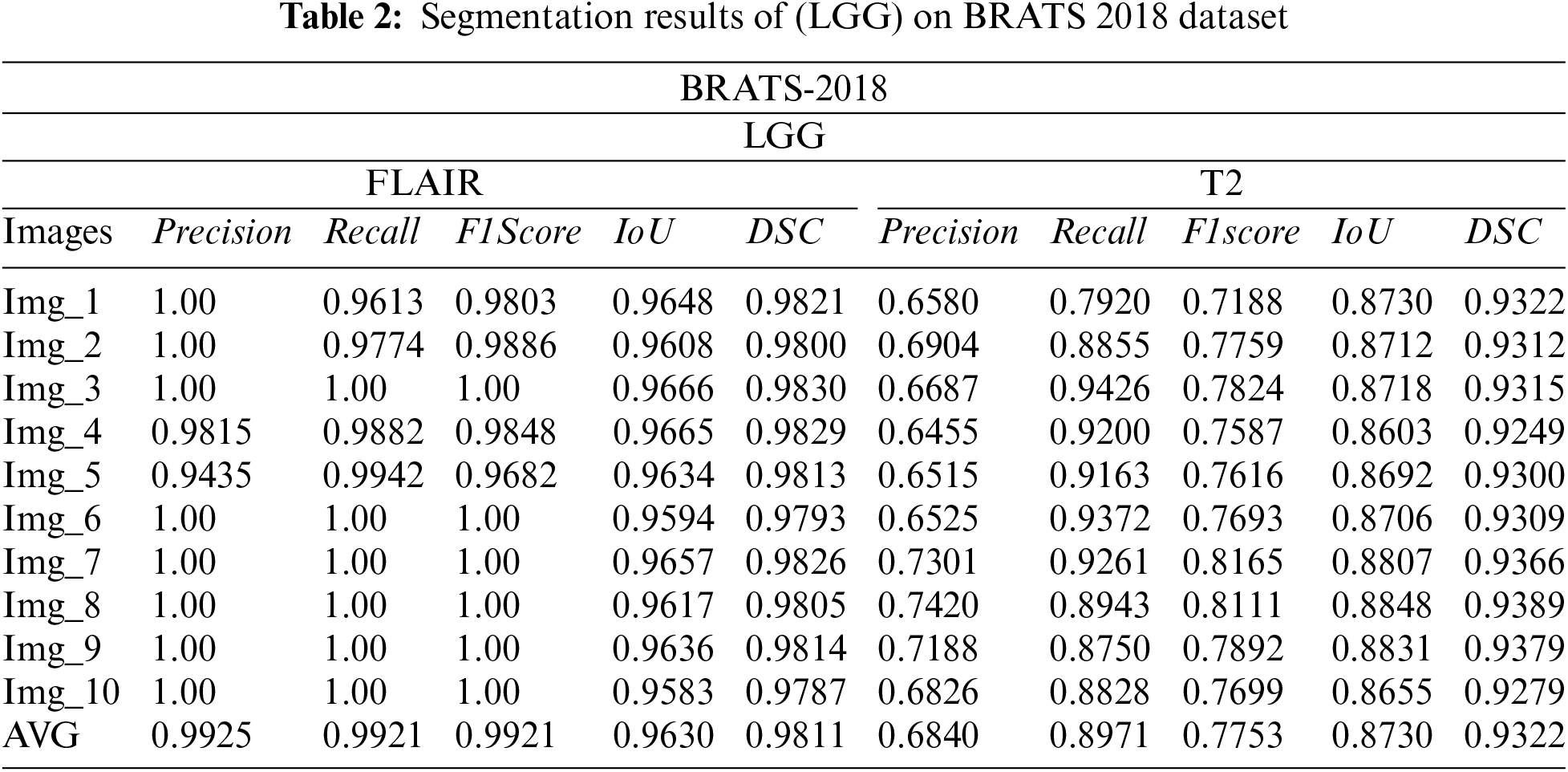
3.1 Segmentation Results on BraTs2018 Dataset
The subsequently, Tabs. 1 and 2 present the results of different performance measures for different sequences of BRATS 2018 dataset. In order to achieve this objective, the dataset is categorized into two classes HGG and LGG. Each class is further subdivided into two sequences that are Flair and T2. We have evaluated the proposed segmentation algorithm on 100 images of each modality. These images are selected randomly from the BRATS 2018 dataset. Afterwards, the top 10 segmentation results are selected that are mentioned in Tabs. 2 and 3. As per aforementioned results, it is concluded that the proposed segmentation algorithm has performed well on LGG-Flair. In this experiment, proposed method has achieved a maximum dice (DSC) of 0.9811. The obtained values of other performance measures Precision, Recall, F1score, and intersection over union (IoU) are 0.9925, 0.9921, 0.9921, and 0.9630 respectively.
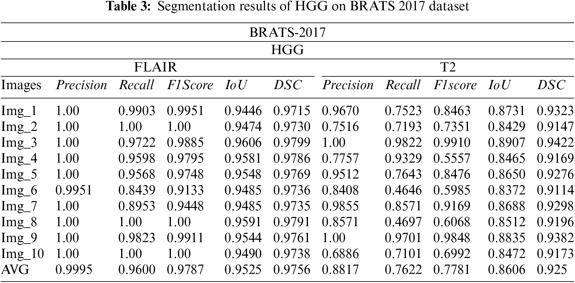
3.2 Segmentation Results on BraTs2017 Dataset
Tabs. 3 and 4 presents the results of different performance measures for different sequences of the BRATS 2018 dataset. From the results, it is concluded that the proposed segmentation algorithm has performed well on LGG-Flair. In this experiment, the proposed method has achieved a maximum DSC of 0.9811. The obtained values of other performance measures Precision, Recall, F1score, and IoU are: 0.9629, 0. 9921, 0. 9766, and 0.9657 respectively. Tab. 5 indicated the comparison of proposed work with existing techniques. It is noticed that the proposed work give us better segmentation results as compared to existing work on the basis of Dice and Jaccard index values.


3.3 Classification Results on BraTs2018 Dataset
The proposed work is evaluated on the basis of some considered performance measures and results are conducted in all SVM classifier named Linear SVM, Quadratic SVM, Cubic SVM, Fine Gaussian SVM, Medium Gaussian SVM and 5 different performance measures such as Accuracy, sensitivity, Spcificity, Precision and time. As far as the classification is concerned four different test are conducted and each test have different features. The data division approach of 60:40 is considered for training and testing for validation of the proposed technique. Also, the 10-fold cross-validation is adopted on all classifier for taking the effective result. Tab. 6 indicate different test cases having there different numbers of features. Afterwards, the top 5 classification results are selected which are given in Tabs. 7–10. In this experiment, the proposed method has achieved a maximum accuracy on cubic SVM 99%, 98.9%, 98.95%, 99% on Test-1, Test-2, Test-3 and Test-4 respectively. It is also noticed that the proposed perform better with regard to classification results when compared to existing work.


Test-1: In Test-1 we used alexnet and inception V3 model having total number of features 4096 and 2048 respectively. However, we only select best 250 feature from both feature set using entropy followed by feature fusion for classification. Among all classifiers, the cubic SVM achieved maximum classification accuracy, sensitivity, specificity and precision that is 99%, 1.0, 1.0, 1.0 respectively. The classification results of cubic SVM are shown in Tab. 7. Moreover, the classification accuracy is also computed on Fine-KNN, enhanced Fine KNN [42], and baggage tree [43]. The results on these classifiers are also better for this experiment.
Test-2: In Test-2 we only select best 500 feature from both feature set using entropy followed by feature fusion for classification. Among all classifiers, the cubic SVM again achieved maximum classification accuracy, sensitivity, specificity and Precision is 98.9%, 0.99, 0.99, 0.99, respectively. The classification results of cubic SVM are shown in Tab. 8.
Test-3: In Test- we only select best 750 feature from both feature set using entropy followed by feature fusion for classification. Among all classifiers, the cubic SVM maintains its supremacy and achieved maximum classification accuracy, sensitivity, specificity and Precision is 98.9%, 0.99, 1.0, 1.0 respectively. The classification results of cubic SVM are shown in Tab. 9.
Test-4: In Test-4 we only select best 1000 feature from both feature set using entropy followed by feature fusion for classification. The cubic SVM finally again performed better and achieved maximum classification accuracy, sensitivity, specificity and Precision is 99%, 0.99, 1.0, 1.0 respectively. The classification results of cubic SVM are shown in Tab. 10.
The proposed work employs the particle Swarm Optimization (PSO) algorithm for brain tumor segmentation to detect ROI from MRI, as well as the deep CNN model for tumor classification. On the BRATS 2018 and 2017 datasets, the proposed work shows the best average segmentation of results using the evaluation metrics DICE and Jaccard Index. The classification is performed on the BRATS 2018 dataset. When compared to existing state-of-the-art methods, the experimental results show that the proposed method outperforms them. The primary goal of the proposed work is to create a novel method for brain tumor segmentation that uses PSO and a deep CNN model for classification in order to reduce false positives while classifying the segmented images into benign and malignant classes. For this reason, MR Images are selected and is enhanced to remove noise and unwanted artifact. Afterwards, the segmentation of tumor is taken out using PSO algorithm. Finally, the post-processing is employed using median filter to extract accurate region of interest (ROI). The proposed technique obtained acceptable segmentation results that are 98.11% and 98.25% of DSC. Also, the proposed method reflects the classification results that are 98.9%, 0.99%, 0.99%, 0.99% correspond to accuracy, sensitivity, specificity and precision respectively. When compared to existing methods, the experimental results show that our proposed work outperforms them. Furthermore, for accurate brain tumour detection and volume calculation, a 3D layered segmentation model is required. The disadvantage of this work is that the threshold value in PSO-based segmentation must be chosen by hand. In the future, neural network techniques will be optimized to obtain higher accuracy while requiring less computational time [44,45].
Funding Statement: This work was supported by “Human Resources Program in Energy Technology” of the Korea Institute of Energy Technology Evaluation and Planning (KETEP), granted financial resources from the Ministry of Trade, Industry & Energy, Republic of Korea. (No. 20204010600090).
Conflicts of Interest: The authors declare that they have no conflicts of interest to report regarding the present study.
References
1. N. Abirami, S. Karthik and M. Kanimozhi, “Automated brain tumor detection and identification using medical imaging,” International Journal of Research in Computer Applications and Robotics, vol. 3, no. 7, pp. 85–91, 2015. [Google Scholar]
2. F. Ullah, S. U. Ansari, M. Hanif and M. A. Ayari, “Brain MR image enhancement for tumor segmentation using 3D U-net,” Sensors, vol. 21, no. 7, pp. 7528, 2021. [Google Scholar]
3. G. K. Seerha and R. Kaur, “Review on recent image segmentation techniques,” International Journal on Computer Science and Engineering, vol. 5, no. 5, pp. 109, 2013. [Google Scholar]
4. M. Nawaz, T. Nazir, M. Masood, A. Mehmood and R. Mahum, “Analysis of brain MRI images using improved cornernet approach,” Diagnostics, vol. 11, no. 2, pp. 1856, 2021. [Google Scholar]
5. M. Sharif, U. Tanvir, E. U. Munir and M. Yasmin, “Brain tumor segmentation and classification by improved binomial thresholding and multi-features selection,” Journal of Ambient Intelligence and Humanized Computing, vol. 4, no. 5, pp. 1–20, 2018. [Google Scholar]
6. D. C. Dhanwani and M. M. Bartere, “Survey on various techniques of brain tumor detection from MRI images,” International Journal of Computational Engineering Research, vol. 4, no. 3, pp. 24–26, 2014. [Google Scholar]
7. Q. Li, Z. Yu, Y. Wang and H. Zheng, “TumorGAN: A multi-modal data augmentation framework for brain tumor segmentation,” Sensors, vol. 20, no. 5, pp. 4203, 2020. [Google Scholar]
8. D. B. Kadam, “Neural network based brain tumor detection using MR images,” Journal of Ambient Intelligence and Humanized Computing, vol. 3, no. 1, pp. 1–18, 2012. [Google Scholar]
9. M. I. Sharif, M. Alhussein, K. Aurangzeb and M. Raza, “A decision support system for multimodal brain tumor classification using deep learning,” Complex & Intelligent Systems, vol. 4, no. 5, pp. 1–14, 2021. [Google Scholar]
10. W. Chen, B. Liu, S. Peng, J. Sun and X. Qiao, “Computer-aided grading of gliomas combining automatic segmentation and radiomics,” International Journal of Biomedical Imaging, vol. 18, no. 4, 2018. [Google Scholar]
11. A. Aziz, U. Tariq, Y. Nam and M. Nazir, “An ensemble of optimal deep learning features for brain tumor classification,” Computers, Materials & Continua, vol. 69, no. 3, pp. 1–15, 2021. [Google Scholar]
12. I. U. Lali, A. Rehman, M. Ishaq, M. Sharif and T. Saba, “Brain tumor detection and classification: A framework of marker-based watershed algorithm and multilevel priority features selection,” Microscopy Research and Technique, vol. 21, no. 2, pp. 1–18, 2019. [Google Scholar]
13. S. Iqbal, M. U. G. Khan, T. Saba and A. Rehman, “Computer-assisted brain tumor type discrimination using magnetic resonance imaging features,” Biomedical Engineering Letters, vol. 8, no. 5, pp. 5–28, 2018. [Google Scholar]
14. M. B. Kulkarni, D. Channappa Bhyri and K. Vanjerkhede, “Brain tumor detection using random walk solver based segmentation from MRI” Microscopy Research and Technique, vol. 20, no. 1, 2018. [Google Scholar]
15. A. Mustaqeem, A. Javed and T. Fatima, “An efficient brain tumor detection algorithm using watershed & thresholding based segmentation,” International Journal of Image, Graphics and Signal Processing, vol. 4, no. 7, pp. 34, 2012. [Google Scholar]
16. P. Kleihues, D. N. Louis, B. W. Scheithauer, L. B. Rorke and G. Reifenberger, “The WHO classification of tumors of the nervous system,” Journal of Neuropathology & Experimental Neurology, vol. 61, no. 21, pp. 215–225, 2002. [Google Scholar]
17. J. A. Schwartzbaum, J. L. Fisher, K. D. Aldape and M. Wrensch, “Epidemiology and molecular pathology of glioma,” Nature Reviews Neurology, vol. 2, no. 5, pp. 494, 2006. [Google Scholar]
18. C. C. Chang and C. J. Lin, “LIBSVM: A library for support vector machines,” LibSVM, vol. 1, no. 1, pp. 1, 2001. [Google Scholar]
19. S. Saritha and N. Amutha Prabha, “A comprehensive review: Segmentation of MRI images—Brain tumor,” International Journal of Imaging Systems and Technology, vol. 26, no. 4, pp. 295–304, 2016. [Google Scholar]
20. I. Njeh, L. Sallemi, I. B. Ayed, K. Chtourou and S. Lehericy, “3D multimodal MRI brain glioma tumor and edema segmentation: A graph cut distribution matching approach,” Computerized Medical Imaging and Graphics, vol. 40, no. 5, pp. 108–119, 2015. [Google Scholar]
21. P. E. Adjei, H. Nunoo-Mensah, R. J. A. Agbesi and J. R. Y. Ndjanzoue, “Brain tumor segmentation using SLIC superpixels and optimized thresholding algorithm,” International Journal of Computer Applications, vol. 975, no. 26, pp. 8887, 2020. [Google Scholar]
22. A. Sehgal, S. Goel, P. Mangipudi, A. Mehra and D. Tyagi, “Automatic brain tumor segmentation and extraction in MR images,” in 2016 Conf. on Advances in Signal Processing (CASP), NY, USA, pp. 104–107, 2017. [Google Scholar]
23. M. U. Akram and A. Usman, “Computer aided system for brain tumor detection and segmentation,” in Int. Conf. on Computer Networks and Information Technology, Toranto, Canada, pp. 299–302, 2011. [Google Scholar]
24. E. Abdel-Maksoud, M. Elmogy and R. Al-Awadi, “Brain tumor segmentation based on a hybrid clustering technique,” Egyptian Informatics Journal, vol. 16, no. 2, pp. 71–81, 2015. [Google Scholar]
25. J. Cheng, W. Huang, S. Cao, R. Yang and W. Yang, “Enhanced performance of brain tumor classification via tumor region augmentation and partition,” PloS one, vol. 10, no. 2, pp. 1–16, 2015. [Google Scholar]
26. M. Havaei, A. Davy, D. Warde-Farley, A. Biard and A. Courville, “Brain tumor segmentation with deep neural networks,” Medical Image Analysis, vol. 35, no. 1, pp. 18–31, 2017. [Google Scholar]
27. M. A. Azam, K. B. Khan, S. Salahuddin, E. Rehmana and S. A. Khan, “A review on multimodal medical image fusion: Compendious analysis of medical modalities, multimodal databases, fusion techniques and quality metrics,” Computers in Biology and Medicine, vol. 144, no. 20, pp. 105253, 2022. [Google Scholar]
28. K. Jabeen, M. Alhaisoni, U. Tariq and A. Hamza, “Breast cancer classification from ultrasound images using probability-based optimal deep learning feature fusion,” Sensors, vol. 22, no. 4, pp. 807, 2022. [Google Scholar]
29. J. Kennedy and R. Eberhart, “Particle swarm optimization (PSO),” in Proc. IEEE Int. Conf. on Neural Networks, Perth, Australia, pp. 1942–1948, 1995. [Google Scholar]
30. H. Y. Zeng, “Improved particle swarm optimization based on tabu search for VRP,” Journal of Applied Science and Engineering Innovation, vol. 6, no. 1, pp. 99–103, 2019. [Google Scholar]
31. T. Hongmei, W. Cuixia, H. Liying and W. Xia, “Image segmentation based on improved PSO,” in 2010 Int. Conf. on Computer and Communication Technologies in Agriculture Engineering, Beijing, China, pp. 191–194, 2010. [Google Scholar]
32. P. Sathya and R. Kayalvizhi, “PSO-based tsallis thresholding selection procedure for image segmentation,” International Journal of Computer Applications, vol. 5, no. 3, pp. 39–46, 2010. [Google Scholar]
33. A. Aqeel, A. Hassan, S. Rehman, U. Tariq and S. Kadry, “A long short-term memory biomarker-based prediction framework for Alzheimer’s disease,” Sensors, vol. 22, no. 7, pp. 1475, 2022. [Google Scholar]
34. F. Afza, M. Sharif, U. Tariq, H. S. Yong and J. Cha, “Multiclass skin lesion classification using hybrid deep features selection and extreme learning machine,” Sensors, vol. 22, no. 11, pp. 799, 2022. [Google Scholar]
35. M. Nawaz, T. Nazir, A. Javed, U. Tariq and H. S. Yong, “An efficient deep learning approach to automatic glaucoma detection using optic disc and optic cup localization,” Sensors, vol. 22, no. 11, pp. 434, 2022. [Google Scholar]
36. S. Bakas, M. Reyes, A. Jakab, S. Bauer and M. Rempfler, “Identifying the best machine learning algorithms for brain tumor segmentation, progression assessment, and overall survival prediction in the BRATS challenge,” Sensors, vol. 20, no. 10, pp. 199, 2020. [Google Scholar]
37. H. Ali, M. Elmogy, E. ALdaidamony and A. Atwan, “MRI brain image segmentation based on cascaded fractional-order darwinian particle swarm optimization and mean shift,” International Journal of Intelligent Computing and Information Sciences, vol. 15, no. 21, pp. 71–83, 2015. [Google Scholar]
38. H. Dong, G. Yang, F. Liu, Y. Mo and Y. Guo, “Automatic brain tumor detection and segmentation using U-net based fully convolutional networks,” in Annual Conf. on Medical Image Understanding and Analysis, New Delhi, India, pp. 506–517, 2017. [Google Scholar]
39. S. Naganandhini and P. Kalavathi, “White matter and gray matter segmentation in brain MRI images using PSO based clustering technique,” Sensors, vol. 21, no. 2, pp. 1–18, 2018. [Google Scholar]
40. J. Amin, M. Sharif, M. Yasmin and S. L. Fernandes, “Big data analysis for brain tumor detection: Deep convolutional neural networks,” Future Generation Computer Systems, vol. 87, no. 2, pp. 290–297, 2018. [Google Scholar]
41. T. W. Ho, H. Qi, F. Lai, F. R. Xiao and J. -M. Wu, “Brain tumor segmentation using U-net and edge contour enhancement,” in Proc. of the 2019 3rd Int. Conf. on Digital Signal Processing, NY, USA, pp. 75–79, 2019. [Google Scholar]
42. B. P. Nguyen, W. L. Tay and C. K. Chui, “Robust biometric recognition from palm depth images for gloved hands,” IEEE Transactions on Human-Machine Systems, vol. 45, no. 16, pp. 799–804, 2015. [Google Scholar]
43. L. Breiman, “Bagging predictors,” Machine Learning, vol. 24, no. 5, pp. 123–140, 1996. [Google Scholar]
44. W. Sun, G. Zhang, X. Zhang, X. Zhang and N. Ge, “Fine-grained vehicle type classification using lightweight convolutional neural network with feature optimization and joint learning strategy,” Multimedia Tools and Applications, vol. 80, no. 1, pp. 30803–30816, 2021. [Google Scholar]
45. W. Sun, X. Chen, X. Zhang, G. Dai and P. Chang, “A multi-feature learning model with enhanced local attention for vehicle re-identification,” Computers, Materials & Continua, vol. 69, no. 2, pp. 3549–3561, 2021. [Google Scholar]
 | This work is licensed under a Creative Commons Attribution 4.0 International License, which permits unrestricted use, distribution, and reproduction in any medium, provided the original work is properly cited. |