| Computers, Materials & Continua DOI:10.32604/cmc.2022.030414 | |
| Article |
Numerical Simulations of One-Directional Fractional Pharmacokinetics Model
1School of Distance Education, Universiti Sains Malaysia, USM Penang, Penang, 11800, Malaysia
2School of Computer Science, Universiti Sains Malaysia, USM Penang, Penang, 11800, Malaysia
*Corresponding Author: Siti Ainor Mohd Yatim. Email: ainor@usm.my
Received: 25 March 2022; Accepted: 09 May 2022
Abstract: In this paper, we present a three-compartment of pharmacokinetics model with irreversible rate constants. The compartment consists of arterial blood, tissues and venous blood. Fick’s principle and the law of mass action were used to develop the model based on the diffusion process. The model is modified into a fractional pharmacokinetics model with the sense of Caputo derivative. The existence and uniqueness of the model are investigated and the positivity of the model is established. The behaviour of the model is investigated by implementing numerical algorithms for the numerical solution of the system of fractional differential equations. MATLAB software is used to plot the graphs for illustrating the variation of drug concentration concerning time. Therefore, the numerical simulations of the model are presented for different values of α which verified the theoretical analysis. Besides, we also observed the pattern of the simulations at the three-compartment of the model by using different values of initial conditions.
Keywords: Pharmacokinetics model; Irreversible rate; Fractional order; Numerical simulations
Physical chemistry is the study of phenomena in a chemical system using the concept of physics. There are several branches related to this field namely thermochemistry, quantum chemistry, electrochemistry, spectroscopy, and chemical kinetics. Chemical kinetic is the understanding of chemical reaction rates widely used in research related to many aspects of cosmology, geology, biology, engineering, and even psychology. In this paper, we focus on the pharmacokinetics model one of the models in the biological field. Pharmacokinetics is a process involving the absorption, distribution, bioavailability, metabolism, and elimination of a drug through the body’s biological systems. Bioavailability is the fraction of a drug absorbed into the systemic circulation, the volume of distribution and refers to measures of the apparent space in the body available to contain the drug, while clearance indicates the body’s ability to eliminate the drug [1].
Various mathematical models have been developed to approximate the concentration of drugs in the body’s system as found in [2–5]. Bischoff et al. [2] studied the mathematics of a two-compartment model based on a well-perfused viscera region and a poorly perfused tissue region which can simulate many of the general features of drug distribution kinetics such as concentration peaks that may occur at short times. The two-compartment model has also been discussed by Feizabadi et al. [6] where the model interacts with dynamic anti-cancer agents. In [4], the model described the mechanisms of how the human body handles the ingestion of nicardipine-cyclodextrin complexes in the gastrointestinal tract (GI), distribution in plasma, and their metabolism in the liver. Hrydziuszko et al. [7] created a two-compartment mathematical model to study cholesterol transport in the circulatory system and its de novo synthesis in the liver. Three compartments of the pharmacokinetic model (drug infusion into, and drug elimination from the central compartment) were studied by [3] because of their complexity and usefulness. Results obtained show that the model required extra computational effort at each data point. Three mathematical models ranging from one-compartment to three-compartment models were established in [8] to understand the distribution of drug administration in the human body through oral and intravenous routes. The models were formulated based on the diffusion process present in Fick’s principle and the law of mass action. Based on the literature, we intend to study the diffusion of drugs in blood and tissue using a three-compartment model [8] which requires the irreversible rate constants as shown in Fig. 1.
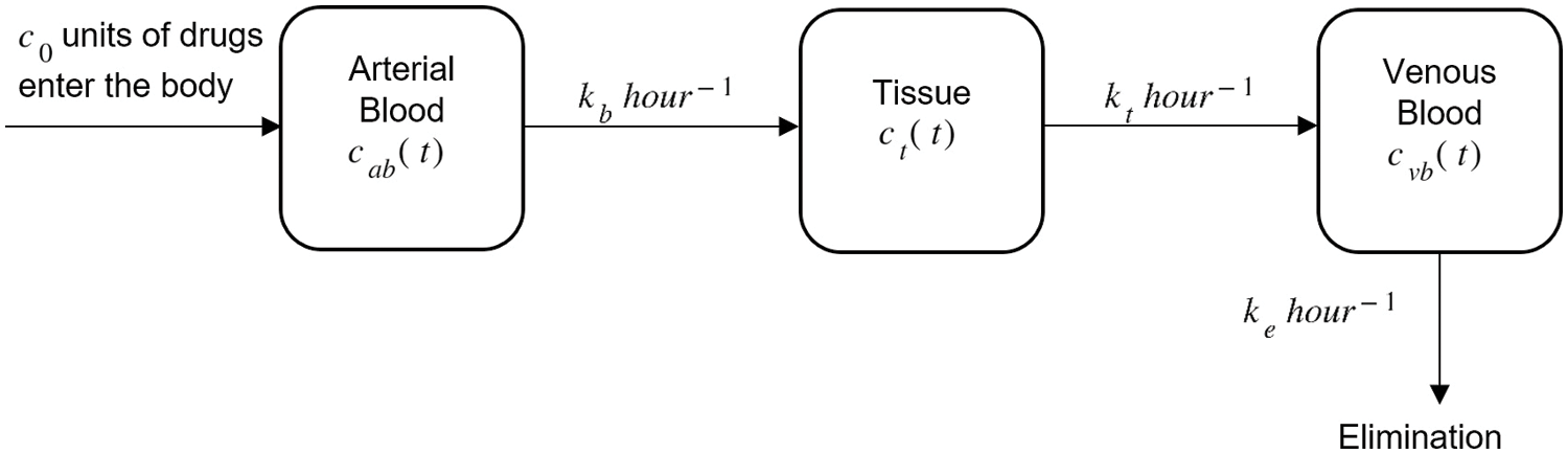
Figure 1: Drug administration through arterial blood, tissue, and venous blood with initial drug intake c0
A principle based on the law of mass conservation known as balance law is applied in the mathematical model (Fig. 1) where
where
where c0 is the initial dosage of drug inserted into the body. The consumption of drugs through arterial blood towards the tissue is assumed to flow at the rate of kb and from the tissue compartment to the venous blood at the rate of kt. Let ke be the drug clearance rate from the venous blood as the level of drug in the venous blood increases with time and ultimately reaches zero when the kidneys and liver excrete the drug from the body.
This paper will present the numerical simulations of the pharmacokinetics model (2) using the generalised fractional order derivatives. According to [9], fractional order calculus is found to be more appealing in modelling a real-world problem in comparison to a classical integer order, as it provides a tool for the description of memory effects and genetic properties of various materials in the recent years. Fractional order differential equations are a generalisation of classical integer order to non-integer order derivative equations, which are used as a basis of mathematical models in physical models, neural networks models, system control models, social networks models, biological models and chaotic systems to investigate the underlying dynamics of the systems [10]. The presence of fractional order derivative in the pharmacokinetics model is necessary as it generalises the results obtained in the case of the standard derivative. The memory effects obtained through fractional order derivatives can measure the concentration rate of drugs in the body. Furthermore, the fractional order system can be adjusted to fit real data by selecting a suitable value of non-integer order to better predict the reaction of the drugs. Thus, some researchers are interested to study the simulations of the fractional pharmacokinetics model [1,11–14]. Some studies concentrate on providing the solutions to the fractional pharmacokinetics model dealing with the Mittag–Leffler, Riemann–Liouville, and Caputo fractional derivatives [15–18]. Therefore, we extend our understanding by modifying the model (2) by incorporating the fractional order α, and the general formula of the fractional three-compartment pharmacokinetic model is formed as follows:
with the following initial conditions
For simplicity [19], Eq. (3) can be rewritten in the form of
The purpose of the study is to investigate the behaviour of the fractional three-compartment pharmacokinetic model (5) since the fractional pharmacokinetics model has only been studied up to a two-compartment model. The model was recently established to characterise the temporal history of pharmaceuticals in the human body that follow an abnormal diffusion mechanism. The three-compartmental fractional model has been proposed and studied to consider different fractional order transmission processes by adopting Caputo’s definition. Thus, this paper is organised as follows: Several definitions related to fractional derivatives will be presented in Section 2. The existence and uniqueness of the mathematical model will be discussed in Section 3. Section 4 will present the positivity of the model and the numerical simulations will be discussed in Section 5. Lastly, a conclusion about this research will be made in Section 6.
There are various definitions of derivative and integration in the literature. Since we are using the approach of Caputo derivative in this paper, the following definitions related to the study are given. The advantage of implementing the Caputo derivative is that the initial conditions for fractional order differential equations with the Caputo derivative are the same for integer differential equations, hence avoiding solvability difficulties and its advantages in applied problems [9]. Besides, many experts choose to utilise the Caputo definition because one may typically have a well-intelligible physical meaning that can be measured when using Caputo's idea [20].
Definition 1. The Riemann-Liouville differential operator of fractional order
where n is the integer defined by
Definition 2. The Caputo differential operator of order
where n is the first integer which is greater than
3 Existence and Uniqueness of the Pharmacokinetics Model
Some qualitative behaviours of the proposed fractional order model (5) are investigated in this section. By considering the following lemma,
Lemma 1. Consider the system
with the initial condition
we begin with the investigation of the existence and uniqueness of the solution (5) in the region
For any
where
4 Positivity of the Pharmacokinetics Model
In this section, the positivity of the solution for the fractional order model (5) is established by considering the following theorem.
Theorem 1. All the solutions of system (5) which start in
Referring to [21], the property of positivity is a fractional differential system (5) satisfying the positivity property for all initial conditions
Establishing the positivity of the solution is important following the fractional order model (5) we have
The integer order case of model (5) can be formed as
where
It follows that
Therefore, the solution of the integer order model with initial conditions
5 Simulations of the Pharmacokinetics Model
In this section, we demonstrate the numerical simulations of
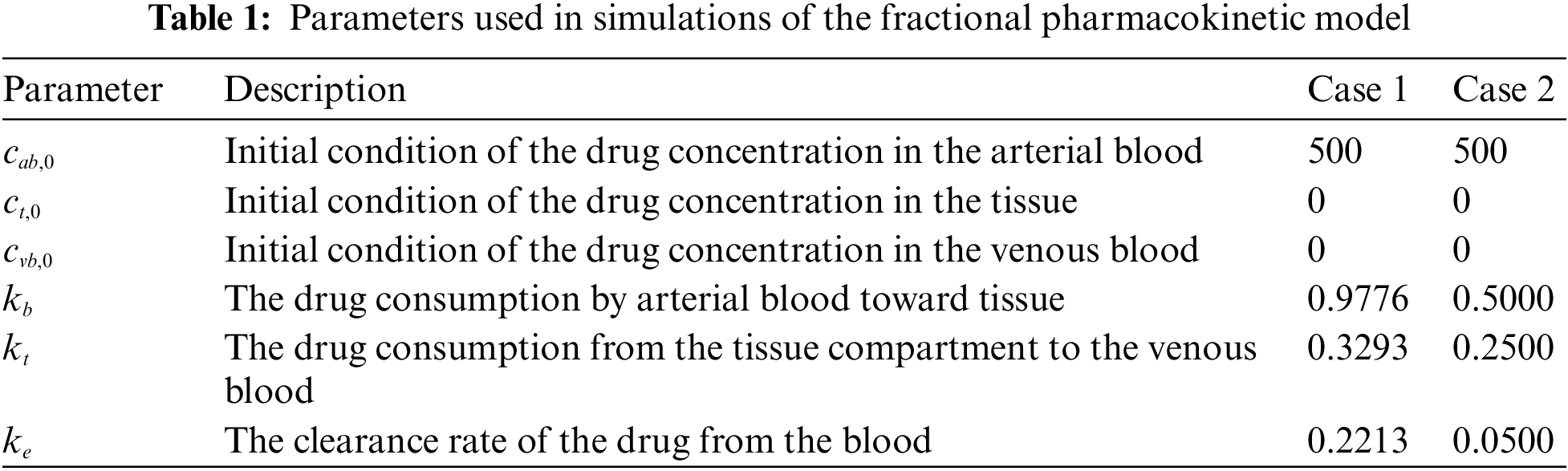
We set
By using MATLAB R2021b, we plot the fractional pharmacokinetics model (5) with a classical integer value of α and the information in Tab. 1 as shown in Fig. 2. Fig. 2a shows the concentration of drugs for Case 1 with the rate constant within
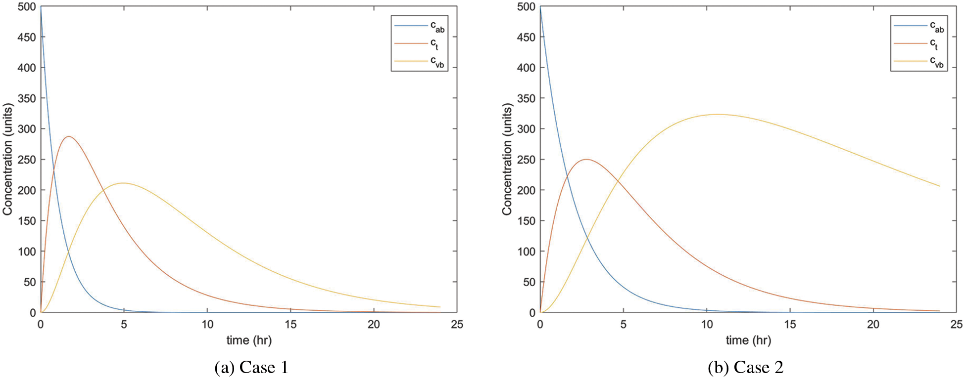
Figure 2: Concentration rate of drugs in three compartments of the body
As mentioned earlier, the different values of α will be considered in this research to illustrate the concentration rate of drugs in
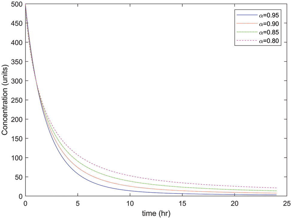
Figure 3: Concentration rate of drugs in arterial blood with different values of α

Figure 4: Concentration rate of drugs in tissue with different values of α

Figure 5: Concentration rate of drugs in venous blood with different values of α
Next, we observe the fractional order pharmacokinetics model (5) by approximating the solutions with α = 0.70 and α = 0.90 as presented in Fig. 6. These figures reveal the pattern of drug distribution in the three-compartment model of the body. We can conclude that the fractional model with α = 0.90 accelerates the absorption of drugs in the body and the full excretion by the kidneys compared to α = 0.70 within 24 h.

Figure 6: Concentration rate of drugs in three parts of the body with α = 0.70 and 0.90
We consider the initial condition of c0 = 200, 300, 400 and 500 to explore the behaviour of the system of the fractional order model (5). As presented in Figs. 7–9, as less drug concentration enters the body, the faster it will be absorbed by the body, thus avoiding an excess of the drug in the body.

Figure 7: Concentration rate of drugs in arterial blood with different values of the initial condition, c0

Figure 8: Concentration rate of drugs in tissue with different values of the initial condition, c0

Figure 9: Concentration rate of drugs in venous blood with different values of the initial condition, c0
In this paper, a fractional order of the three-compartment pharmacokinetic model (5) was proposed and studied. The existence and uniqueness of the solution of model (5) were examined under sufficient conditions. Non-negativity of the solution of the fractional order model (5) was conducted. Numerical simulations were presented to analyse the behaviour of the fractional order model (5). Then, we analysed the quantitative behaviour using different values of the rate constant and a few values of
Acknowledgement: The authors would like to thank the editor and reviewers for the constructive comments and useful suggestions, which improved the manuscript.
Funding Statement: This work was supported by Fundamental Research Grant Scheme Universiti Sains Malaysia, 203/PPSK/203.6712025.
Conflicts of Interest: The authors declare that they have no conflicts of interest to report regarding the present study.
References
1. A. Ahmadian, N. Senu, F. Larki, S. Salahshour, M. Suleiman et al., “Numerical solution of fuzzy fractional pharmacokinetics model arising from drug assimilation into the bloodstream,” Abstract and Applied Analysis, vol. 2013, no. 2, pp. 1–17, 2013. [Google Scholar]
2. K. B. Bischoff and R. L. Dedrick, “Generalized solution to linear, two-compartment, open model for drug distribution,” Journal of Theoretical Biology, vol. 29, no. 1, pp. 63–83, 1970. [Google Scholar]
3. J. R. Jacobs, “Analytical solution to the three-compartment pharmacokinetic model,” IEEE Transactions on Biomedical Engineering, vol. 35, no. 9, pp. 763–765, 1988. [Google Scholar]
4. S. Shityakov and C. Förster, “Pharmacokinetic delivery and metabolizing rate of nicardipine incorporated in hydrophilic and hydrophobic cyclodextrins using 2 compartment mathematical model,” The Scientific World Journal, vol. 2013, no. 7, pp. 1–9, 2013. [Google Scholar]
5. S. Chomcheon, Y. Lenbury and W. Sarika, “Stability, hopf bifurcation and effects of impulsive antibiotic treatments in a model of drug resistance with conversion delay,” Advances in Difference Equations, vol. 2019, no. 274, pp. 1–18, 2019. [Google Scholar]
6. M. S. Feizabadi, C. Volk and S. Hirschbeck, “A two-compartment model interacting with dynamic drugs,” Applied Mathematics Letters, vol. 22, no. 8, pp. 1205–1209, 2009. [Google Scholar]
7. O. Hrydziuszko, A. Wrona, J. Balbus and K. Kubica, “Mathematical two-compartment model of human cholesterol transport in application to high blood cholesterol diagnosis and treatment,” Electronic Notes in Theoretical Computer Science, vol. 306, no. 9493, pp. 19–30, 2014. [Google Scholar]
8. M. A. Khanday, A. Rafiq and K. Nazir, “Mathematical models for drug diffusion through the compartments of blood and tissue medium,” Alexandria Journal of Medicine, vol. 53, no. 3, pp. 245–249, 2017. [Google Scholar]
9. N. I. Hamdan and A. Kilicman, “A fractional order sir epidemic model for dengue transmission,” Chaos Solitons and Fractals, vol. 114, no. 2, pp. 55–62, 2018. [Google Scholar]
10. M. Moustafa, M. H. Mohd, A. I. Ismail and F. A. Abdullah, “Dynamical analysis of a fractional order eco-epidemiological model with nonlinear incidence rate and prey refuge,” Journal of Applied Mathematics and Computing, vol. 65, no. 1-2, pp. 623–650, 2021. [Google Scholar]
11. A. Dokoumetzidi and P. Macheras, “Fractional kinetics in drug absorption and disposition processes,” Journal of Pharmacokinetics and Pharmacodynamics, vol. 36, no. 2, pp. 165–178, 2009. [Google Scholar]
12. I. Petráš and R. L. Magin, “Simulation of drug uptake in a two compartmental fractional model for a biological system,” Communications in Nonlinear Science and Numerical Simulation, vol. 16, no. 12, pp. 4588–4595, 2011. [Google Scholar]
13. D. Copot, A. Chevalier, C. M. Ionescu and R. D. Keyser, “A Two-compartment fractional derivative model for propofol diffusion in anesthesia,” in IEEE Multi-Conference on Systems and Control, 28–30 August, Hyderabad, India, pp. 264–269, 2013. [Google Scholar]
14. Y. Qiao, H. Xu and H. Qi, “Numerical simulation of a two-compartmental fractional model in pharmacokinetics and parameters estimation,” Mathematical Methods in the Applied Sciences, vol. 2021, no. 14, pp. 1–11, 2021. [Google Scholar]
15. D. Verotta, “Fractional dynamics pharmacokinetics-pharmacodynamic models,” Pharmacokinet Pharmacodyn, vol. 37, no. 3, pp. 257–276, 2010. [Google Scholar]
16. J. K. Popovic, D. Dolicanin, M. R. Rapaic, S. L. Popovic, S. Pilipovic et al., “A nonlinear two compartmental fractional derivative model,” European Journal of Drug Metabolism and Pharmacokinetics, vol. 36, no. 4, pp. 189–196, 2011. [Google Scholar]
17. J. K. Popovic, D. T. Spasic, J. Tosic, J. L. Kolarovic, R. Malti et al., “Fractional model for pharmacokinetics of high dose methotrexate in children with acute lymphoblastic leukaemia,” Communications in Nonlinear Science and Numerical Simulation, vol. 22, no. 1–3, pp. 451–471, 2015. [Google Scholar]
18. P. Sopasakis, H. Sarimveis, P. Macheras and A. Dokoumetzidis, “Fractional calculus in pharmacokinetics,” Journal of Pharmacokinetics and Pharmacodynamics, vol. 45, no. 1, pp. 107–125, 2018. [Google Scholar]
19. J. Singh, D. Kumar and D. Baleanu, “On the analysis of chemical kinetics system pertaining to a fractional derivative with mittag-leffler type kernel,” American Institute of Physics, vol. 27, no. 10, pp. 103113, 2017. [Google Scholar]
20. N. A. Zabidi, Z. A. Majid, A. Kilicman and Z. B. Ibrahim, “Numerical solution of fractional differential equations with Caputo derivative by using numerical fractional predict-correct technique,” Advances in Continuous and Discrete Models, vol. 2022, no. 26, pp. 1–23, 2022. [Google Scholar]
21. J. Cresson and A. Szafrańska, “Discrete and continuous fractional persistence problems-the positivity property and applications,” Communications in Nonlinear Science and Numerical Simulation, vol. 44, no. 3, pp. 424–448, 2017. [Google Scholar]
22. K. Diethelm and A. D. Freed, “The fracPECE subroutine for the numerical solution of differential equations of fractional order,” Forschung und wissenschaftliches Rechnen, vol. 1999, pp. 57–71, 1998. [Google Scholar]
23. R. Garrappa, “Trapezoidal methods for fractional differential equations: Theoretical and computational aspects,” Mathematics and Computers in Simulation, vol. 11, no. 172, pp. 96–112, 2015. [Google Scholar]
24. S. Chakraverty, S. Tapaswini and D. Behera, “Fuzzy differential equations and applications for engineers and scientists. Boca Raton, Florida: CRC Press, 2016. [Online]. Available: https://www.taylorfrancis.com/books/mono/10.1201/9781315372853. [Google Scholar]
 | This work is licensed under a Creative Commons Attribution 4.0 International License, which permits unrestricted use, distribution, and reproduction in any medium, provided the original work is properly cited. |