| Computers, Materials & Continua DOI:10.32604/cmc.2022.030420 | |
| Article |
Residual Autoencoder Deep Neural Network for Electrical Capacitance Tomography
1Department of Computer Science in Jamoum, Umm Al-Qura University, Makkah, 25371, Saudi Arabia
2Computers and Systems Engineering Department, Mansoura University, Mansoura, 35516, Egypt
3Laboratoire D’Informatique et des Technologies de L’Information D’Oran (LITIO), University of Oran, 31000, Oran, Algeria
*Corresponding Author: Wael Deabes. Email: wadeabes@uqu.edu.sa
Received: 25 March 2022; Accepted: 15 June 2022
Abstract: Great achievements have been made during the last decades in the field of Electrical Capacitance Tomography (ECT) image reconstruction. However, there is still a need to make these image reconstruction results faster and of better quality. Recently, Deep Learning (DL) is flourishing and is adopted in many fields. The DL is very good at dealing with complex nonlinear functions and it is built using several series of Artificial Neural Networks (ANNs). An ECT image reconstruction model using DNN is proposed in this paper. The proposed model mainly uses Residual Autoencoder called (ECT_ResAE). A large-scale dataset of 320 k instances have been generated to train and test the proposed ECT_ResAE model. Each instance contains two vectors; a distinct permittivity distribution and its corresponding capacitance measurements. The capacitance vector has been modulated to generate a 66×66 image, and represented to the ECT_ResAE as an input. The scalability and practicability of the ECT_ResAE network are tested using noisy data, new samples, and experimental data. The experimental results show that the proposed ECT_ResAE image reconstruction model provides accurate reconstructed images. It achieved an average image Correlation Coefficient (CC) of more than 99% and an average Relative Image Error (IE) around 8.5%.
Keywords: ECT; image reconstruction; deep learning; residual; autoencoder; IE; CC
Electrical capacitance tomography (ECT) is a measurement technique that allows the multiphase flow process to be observed by the generation of its cross-sectional image [1]. Generally, the use of ECT is required to study multiphase dielectric flow processes, in various fields, such as pneumatic conveying systems as well as fluidized beds [2,3]. The ECT system is made up of three parts, which are a capacitance sensor, an electronic data acquisition, and a post-processing imaging computer. To simplify, the principle of the ECT is to measure the capacitance between the electrodes around the imaging area and then calculate the permittivity distribution based on the relationship between permittivity and capacitance. The process of generating a permittivity distribution from the measured capacitance is called ECT image reconstruction, since the permittivity distribution is presented in the form of a cross-sectional image. The problem of ECT image reconstruction is a challenging task because of the nonlinear relationship that exists between the capacitance and permittivity. Approaches based on a simplified linear model consist of non-iterative and iterative algorithms [4]. Non-iterative methods are fast and simple, and can therefore be applied for linear imaging, but the quality of the reconstructed images remains limited. Linear Back Projection (LBP) [5] is a common non-iterative method, but it contains drawbacks such as large artifacts in processing complex media distribution and missing edges. Iterative methods, such as Tikhonov regularization [6], Iterative Landweber Method (ILM) [7], and the Total Variation-based Regularization (TVR) [8], produce better image quality but generally require more computation time. Furthermore, image reconstruction algorithms, based on the nonlinear model [9], have a superior quality of image reconstruction which, however, requires intensive calculations and only meets the requirements of online imaging at a minimum for certain ECT applications. Therefore, they are generally only used for offline imaging and analysis.
As a result, there is a crucial need to find a new method to improve results of image reconstruction and speed up the reconstruction process. Recently, Machine Learning (ML) techniques are flourishing and used in many fields [10]. The most important interest of ML is that it gives the machine the ability to learn algorithms without strict orders from different programs or from limited instructions [11]. Most notably, interest has been focused on Deep Learning (DL) based on several sets of Artificial Neural Network (ANN) capable of mapping fairly complex nonlinear functions [12–14]. ANN provide robust models and are used in a number of different applications [15–17]. Classification and pattern recognition are achieved by DL from using many layers for nonlinear data processing of supervised or unsupervised feature extraction [18]. Emulation of the approach that allows the human brain to perform feature extraction directly from unsupervised data is the main goal of DL. Due to the unrecognized nature of image composition, standard ML techniques do not work well with images if run directly. DL techniques enable features automatic extraction from image reconstruction [19].
The use of intelligent methods has double advantages; it allows avoiding the computation of the sensitivity matrix in the forward problem of the ECT. It also allows to avoid the linearization of the inverse problem of ECT image reconstruction. In ECT image reconstruction, ANN offer the current state-of-the-art nonlinear approach, that generally offer efficiency and robustness. Researchers from the ECT area tried to use machine learning-based approaches to solve the problem of image reconstruction. Deabes et al. solved the forward problem using NN system, and they proposed a Multi-Fuzzy System (MFS) to generate images of conductive materials in a Lost Foam Casting (LFC) process [20,21].
Deep Neural Networks (DNN) have been widely used in many fields but they are more suited for initial data post-processing. DNN have, generally, a very powerful ability for learning arbitrary nonlinear complex functions because they use multiple hidden layers. One of the advantages of DNN is the possibility it gives computers to perform complex calculations based on simpler calculations in order to optimize the efficiency of the computer. Convolutional Neural Networks (CNN) are a particular category of DNN. The information on the planar structure is better preserved and the features are obtained by a filter. Therefore, they are more specifically suited to the imaging field. To solve several inverse problems in imaging process, training a CNN which enhances the informational content of the reconstructed image, has been widely used. Among these inverse problems, we refer the reader to Photoacoustic Tomography (PAT) [22,23], Electrical Impedance Tomography (EIT) [24], Computed Tomography (CT) [25,26], and Magnetic Resonance Imaging (MRI) [27].
Using DNN techniques allow to speed up the extraction of industrial process parameters and improve the ECT image reconstruction process [28]. The DNN algorithms used have been transferred and adapted such as in image reconstruction methods based on CNN [29], multi-scale CNNs [30], Dbar methods [31], and autoencoder [32]. The problem of ECT image reconstruction was also addressed by Li et al. using the BP and RBF neural networks [33]. Deabes et al. developed a highly reliable Long-Short Term Memory (ECT-LSTM-RNN) model to image the metal during the LFC industrial process [34]. Also, an LSTM-IR algorithm is implemented to map the capacitance measurements to accurate material distribution images [35].
From this perspective, we propose an ECT Residual Autoencoder (ECT_ResAE) neural network to explore a new methodology, based on DNN, which allows ECT image reconstruction. The autoencoder can better extract image edge information through its unique parameter extraction capability. This paper therefore applies the improved autoencoder to ECT image reconstruction on this basis. Applications such as image-to-image translation [36], Super-Resolution [37], image painting [38], and rain removal [39] have widely applied autoencoder architectures. To solve the problem of performance degradation as the number of layers increases, He et al. [40], from Microsoft Research Institute, proposed the concept of Residual Network (ResNet) within the framework of residual learning. Results obtained using ResNets outperformed those obtained using common CNNs in object recognition and image classification [41,42]. ResNets depth is deeper than traditional CNNs due to residual learning, which allows them to give better results and extract more critical features.
The proposed ECT_ResAE model has an encoder and decoder networks with four layers each, which can solve the inverse problem of the ECT. The learning step allows to extract the features of each layer, one after the other, then to match the features of the original spatial data to a new space. During the learning step, a nonlinear mapping relationship is established between the internal permittivity distribution and the boundary measured capacitance of the object. The ECT image reconstruction is then performed by direct estimation of the corresponding permittivity distribution. The results obtained from simulations and experiments show that the reconstructed images are of satisfying quality and the proposed ECT_ResAE model has good generalization ability.
The paper is organized as follows. In Section 2, The ECT model is explained. The residual autoencoder model for ECT problem is discussed in Section 3. The generated ECT dataset is presented in Section 4. Section 5 will be dedicated to the presentation of the experimental results of image reconstruction using the ECT_ResAE. Finally, Section 6 is devoted to the conclusion.
Practically, as shown in Fig. 1, the ECT sensor contains n = 12 electrodes evenly mounted around the field uniform [43]. The number of all independent measured mutual capacitance is M = n(n−1)/2, M = 66 area of interest. Insulating guards between electrodes decrease the external coupling, and keep the electric in this case.
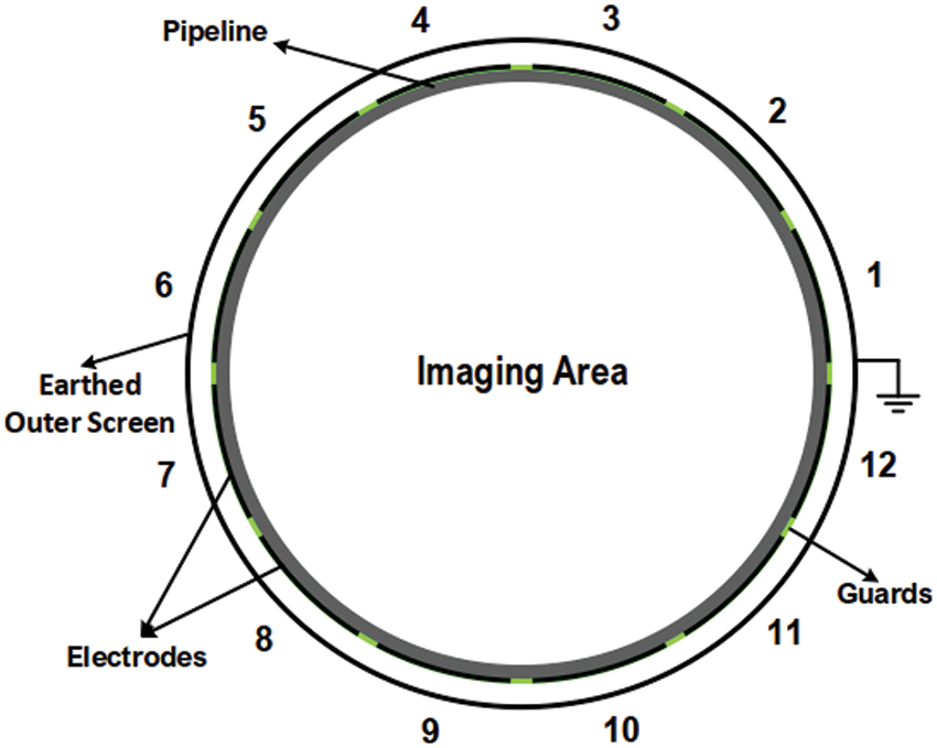
Figure 1: Cross-sectional view of ECT sensor
The ECT forward problem for calculating the capacitance measurements of certain material distribution is solved using Finite Element Method (FEM). The imaging area is divided into small triangle elements with N = 12932 nodes. Accordingly, the ECT forward problem is numerically solved to calculate the capacitance as Eq. (1):
where C is the capacitance vector, M is the number of measurements, S is the sensitivity matrix, N is the number of image’s pixels, and G is the permittivity distribution.
The ECT is classified as an ill-posed problem (N >> M), where the reconstructed image can intensely be affected by any small error in the capacitance measurements. The LBP method, Eq. (2), is simple, and non-iterative image reconstruction algorithm, but it generates poor quality images.
While applying iterative algorithms, such as ILM in Eq. (3), potentially enhances the image quality, but it requires vast computational resources.
where
3 ECT Residual Autoencoder (ECT_ResAE) Model
The structure of the proposed ECT_ResAE model for solving the ECT inverse problem is described here, as well as the basic theory of the autoencoder network with a residual block. Fig. 2 shows the architecture of the proposed ECT_ResAE model, where the model has two stages, pre-processing and deep learning phases, respectively.
In the pre-processing phase, the input capacitance vector
Modulator
There are M = 66 capacitance measurements produced as a raw vector from the ECT sensor shown in the ECT sensor electrodes CCW rotation. This rotation step is repeated
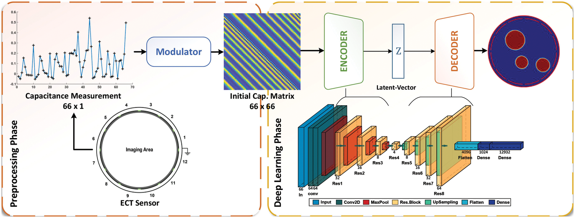
Figure 2: Architecture of ECT Residual Autoencoder (ECT_ResAE) model
The residual autoencoder (ResAE) model is implemented in this phase. The ResAE takes the modulated capacitance matrix and outputs the final ECT permittivity distribution image. The basic theory of the autoencoder network with a residual block is explained hereafter.
3.2.1 Conception of the Autoencoder
The main objective of an autoencoder is features detection. It is specifically used in order to reconstruct an advanced representation of the input data, this by learning their corresponding compressed representation. Generally, the autoencoder model consists of three parts: the encoder for extracting features from n-dimensional input (In our case
The model has one input layer, a network layer is denoted by each block, the abstraction of the connection from one layer to another one is represented by an arrow, and the depth of this layer is denoted by the number under each block. The input enters the encoder through convolutional layer, then Residual Blocks (RB) [44], and Max pooling layers, which are alternately arranged. The function of pooling layers is to down sampling feature maps. The pooling layers works by summarizing the presence of features in patches of the feature map, and the most activated presence of a feature, respectively. Max pooling layers rather than average pooling are adopted to gain better performance. The decoder part consists of a sequence of upsampling layers followed by residual blocks, then the output is flattened, and it goes through two fully connected layers with the last one of size
Compared to common DNN techniques, ResNets introduced residual learning into the DNN construction. The final results are very much influenced by the depth of the DNN, so deeper networks are usually constructed. However, the network depth increase can be the source of the gradient explosion phenomenon, and the network performance degradation. According to literature results [45], the simple fact of adding pooling and convolution layers to the network does not help in improving the network accuracy but rather conducts to a degradation of the network performance. In this paper, to solve the above problem, we use residual learning. Residual represents the residual difference between the local input (x) and output (g(x)), Eq. (4)
In residual learning, the learning objective is 0 unlike what is done in identity mapping. In Fig. 3, the residual block applied in the ECT_ResAE model is illustrated. Since the objective is the reduction of the difference between the input and the output, so that the original input is directly connected to one particular network layer, which allows the network to learn the residual. Residual learning is obtained through a fast connection between the input and the output of a block. It effectively trains the network parameters and ensures performance while the network can learn more in-depth features, besides avoiding adding supplementary parameters and calculations to the network.
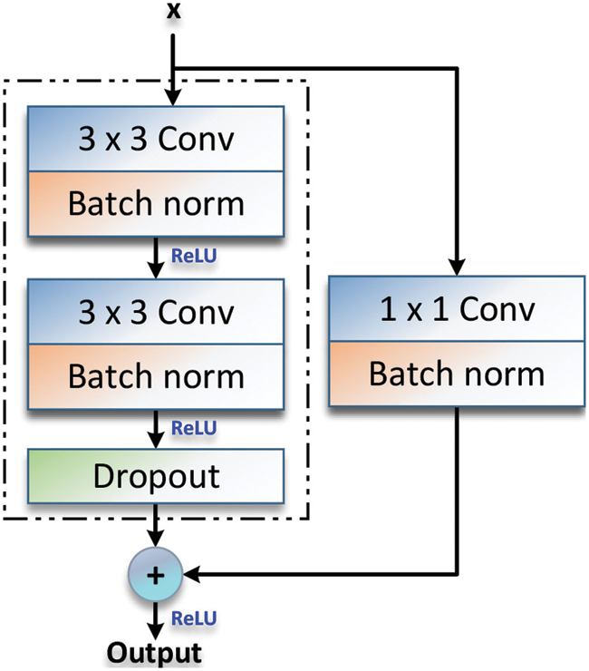
Figure 3: Structure of residual block
The traditional layer is fully connected, so it is different from the convolutional layer. In the convolutional layer, the input of each node is only a small component of the upper layer of the neural network called the nucleus or filter. The filter can transform a sub node matrix of neural network. The convolution is given by Eq. (5).
where the activation function is represented by f,
3.2.4 Batch Normalization (BN) Layers
During DNN learning, the distribution of the inputs of the next layer will change, depending on the change of the parameters of the previous layer, therefore the learning of deeper neural networks becomes more difficult. In the training process of the ECT_ResAE model, batch normalization, provides a solution to the difficulty of networks training. It allows the input of each layer to keep the same distribution, thus avoiding the overfitting and effectively improve the learning speed of networks. The input data are made up in batches, for example, we set the “batch_size” parameter to 250; thus 250 data items will be entered as a batch at the same time. In order for the data distribution to remain unchanged, the BN layers must normalize each batch. The BN layer, through the application of a transformation, keeps the output standard deviation close to 1 and the mean output close to 0.
Consider the batch of inputs
The batch normalization output is given by
where
3.2.5 Activation and Dropout Layers
In the proposed ECT_ResAE model, ReLU has been chosen as an activation function, as expressed in Eq. (9),
ReLU calculates the activation value based on a threshold rather than complicated operations. Moreover, since its derivative is always equal to 1, it is considered as not saturating. The scalability of the proposed model is improved by adding a dropout layer, which has been shown to be very efficient in training large dataset. The network can learn more robust features by randomly discarding half of neurons from the network during the training process.
To optimize the ECT_ResAE model’s parameters, the optimization algorithm must minimize the average reconstruction error Eq. (10),
where the loss function is represented by L. The Gradient Descent method allows updating the weight matrices and the bias vectors according to formulas (11), and (12).
where
For training and testing purposes, a large-scale ECT simulation dataset has been created by a developed Matlab software package. Different types of two phases flow patterns have been implemented, as well as their corresponding capacitance measurements can be accurately calculated. The ECT dataset has pairs of permittivity distribution vector, and its equivalent capacitance measurements vector. The sensor’s PVC pipe of the ECT sensor, shown in Fig. 1, has a relative permittivity 2. The pipe has a 126 mm diameter, and a thickness of 2.5 mm. The electrodes are evenly mounted around the pipe with a span angle of each electrode is 26◦, and separation gaps of 4◦. The developed ECT dataset has 320k instances of nine flow patterns, 10k ring patterns, annular with 20k patterns, 10k stratified patterns, 140k patterns divided between one, two, and three circular bars, and 140k patterns of 1 to 3 square bars, as shown in Fig. 4. This figure illustrates samples of different input modulated capacitance matrix and their corresponding ground truth flow patterns. The high permittivity phase is assigned to 4 (like glass rods), where the low permittivity phase assigned to 1 (like air).
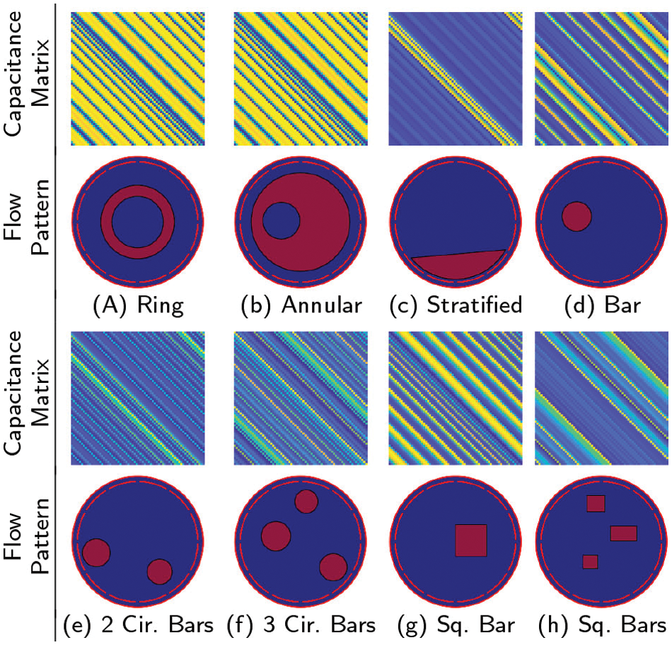
Figure 4: Samples of different input modulated capacitance matrix and ground truth flow patterns
Random variables are used in building the dataset to make it more inclusive. For sample, the ring’s width for annular flow is randomly changed between 10%–95% of the radius of the imaging area. The stratified flow’s height is assigned to a random variable in a range of 5%–95% of the diameter of the sensing field. The number of the circular and square bars varied from 1 to 3.
The process of developing the ECT_ResAE model starts by training the residual autoencoder DNN using the developed ECT dataset. The performance of the proposed model is tested based on reconstruction results of the testing dataset. A validation process is usually run during the training phase to avoid the over- fitting problem. A random 10% of training samples are chosen each epoch of the training process to validate the model. The overall model’s performance and its generalization ability are tested based on the equivalent performance on the original dataset, noisy testing data, new data not included in the training patterns, and real experimental data.
Typically, in the ECT problem two mutual measures, a relative Image Error (IE) and a Correlation Coefficient (CC), are applied to assess the image quality, and reconstruction algorithm’s performance [46]. The IE and CC measures the spatial differences between the true and reconstructed patterns. Eq. (13) shows the relative IE,
where
The similarity between the reconstructed and real images is evaluated by the CC in Eq. (14),
where
TensorFlow ML platform [47], and Keras DL API [48] are used to implement the training and testing phases of the ECT_ResAE model. During the testing phase, a modulated capacitance matrix of size
5.2 Qualitative Analysis on Testing Patterns
A testing dataset of ratio 30% of 320k patterns of the ECT simulation dataset is randomly chosen to assess reconstruction and generalization abilities of the proposed ECT_ResAE model. The model has not seen this testing set during the training phase. The loss curves, shown in Fig. 5, decay over 250 epochs for the training and validation sets.
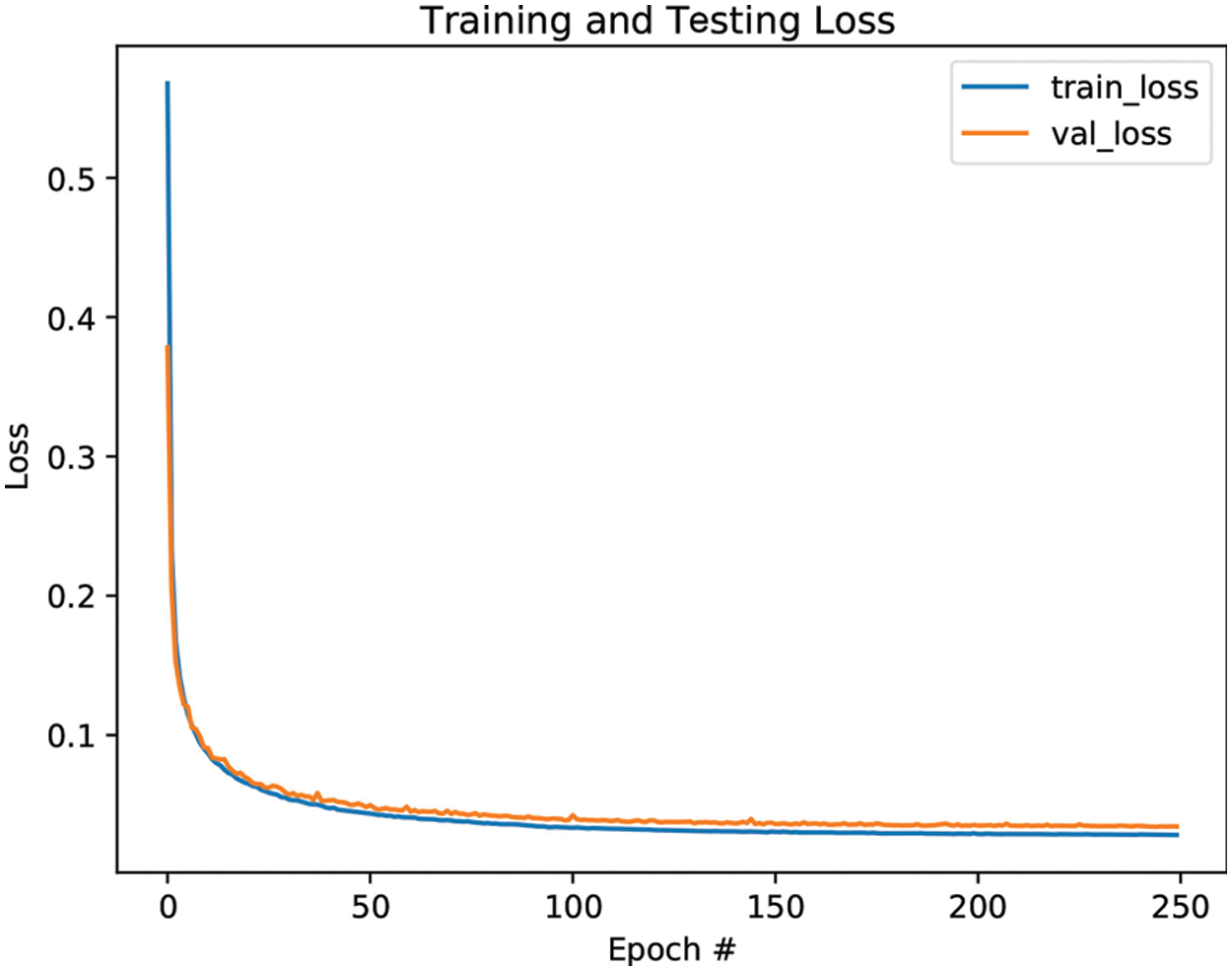
Figure 5: Training and validation loss curves
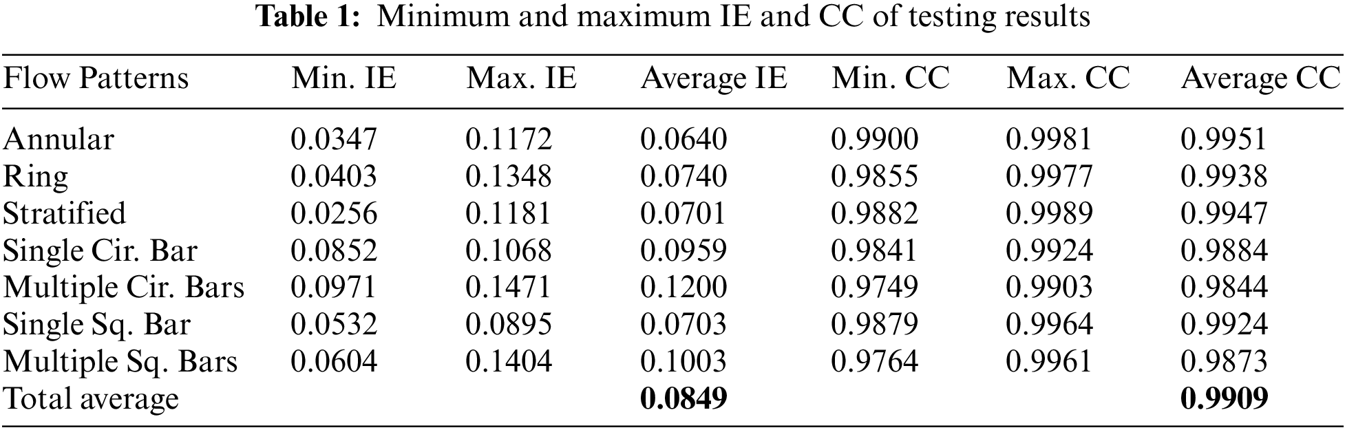
The minimum, maximum, and average values of the relative IE and CC are listed in the Tab. 1 for each two-phase flow type in the testing set. These results prove that the ECT_ResAE model can generate accurate images with high correlation to real permittivity patterns. The overall performance of the proposed ECT_ResAE model is excellent since the average values of the IE and CC are 0.0849 and 0.9909, respectively. The stated results show that the average CC values of most of the flow types exceed 99%, and the IE’s values are less than 10% except the multiple circular and square bars flow type. Also, the relative IE and CC values of the annular flow types are the best compared with the other.
The IE and CC box plots of all the testing patterns are drown in Figs. 6 and 7, respectively. The maximum and minimum values of each flow type listed in Tab. 1) are represented by the upper and lower limits, while the red line is the median. The IE and CC, shown in Figs. 6 and 7, are in reasonable intervals, which confirms the high performance of the ECT_ResAE model.

Figure 6: Box plots of relative image errors (IE)
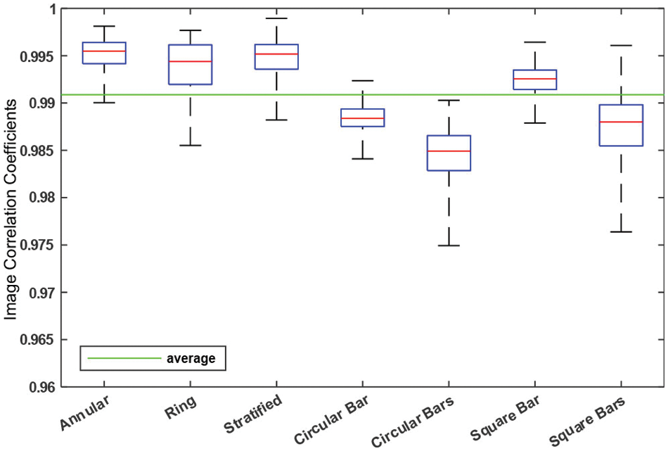
Figure 7: Box plots of Corr. Coeff. (CC)
Examples of reconstructed images with minimum and maximum CC values of each flow type listed in Tab. 1 are shown in Fig. 8. Visually, the reconstructed images that have minimum CC are very correlated to the real flow patterns, although the generated images that have maximum CC of course have a better visual effect. As well, images with high CC are classified as high phase ratio flows, however the reconstructed images with low CC have low phase ratio, but circular bars flow. Generally, ECT_ResAE model executes well on the testing patterns, and it powerfully can create images of all typical flow types with correctly predicting material’s permittivity values.

Figure 8: Examples of min. and max. CC image reconstruction results
An experiment using variety of flow patterns is designed to compare the performance of the proposed ECT_ResAE model with other traditional and DNN image reconstruction algorithms. The results are shown in Fig. 9, where the real phantom is in the first column, the second column contains the modulated capacitance matrix of each phantom, and the others show the results from the LBP, iterative Tikhonov, ILM, CNN [30], LSTM-IR [35], and ECT_ResAE algorithms, respectively. The hyperparameters of the Tikhonov regularity algorithm are selected by try and error procedure. The optimal regularization parameter is selected 0.01, while the iteration numbers of the Tikhonov and the ILM are 200 and 1000 iterations, respectively. The LBP algorithm generates the input images for the CNN algorithm. The ECT_ResAE model generates more accurate images compared with the other algorithms. Moreover, the objects in the ECT_ResAE re- constructed images have sharp edges without transition zone. Tab. 2 states the IE and CC values of all reconstruction algorithms. The ECT_ResAE model outperforms the other reconstruction algorithms. Bars Figs. 10a and 10b represent the IE and CC results in Tab. 2.
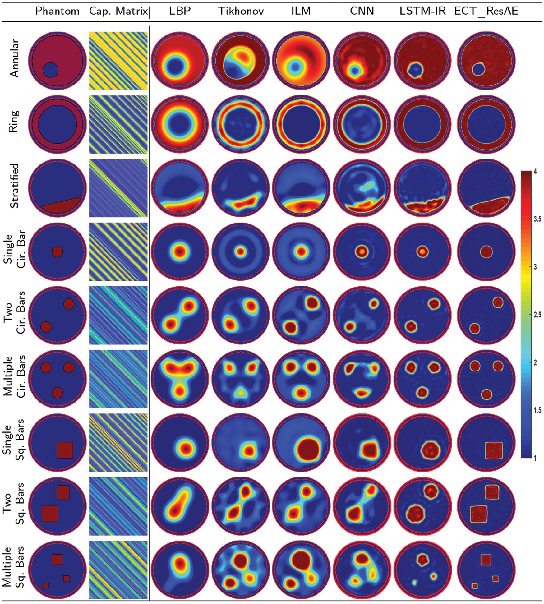
Figure 9: Reconstructed images of well-known image reconstruction algorithms
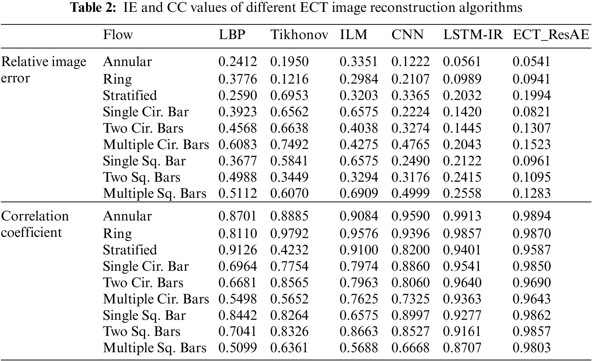
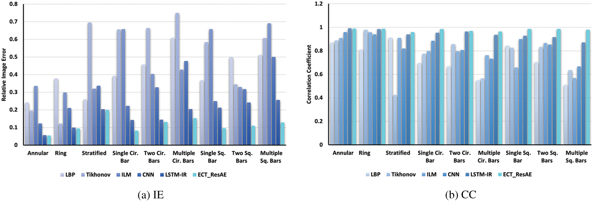
Figure 10: Comparison of IE and CC values of various ECT reconstruction algorithms
In the ECT system, noise is a combination of several different sources such as capacitance measurements circuit, communication between electrodes and host computer (analogue transmission line), external electrical fields and stray capacitance. To assess the robustness of the proposed ECT_ResAE model, a noisy data is applied during the training and testing processes. The capacitance input vectors of the ECT dataset are contaminated by a gaussian noise of Signal_to_Noise_Ratio (SNR = 30 dB) before the modulation step. The value of SNR = 30 dB is selected since this value is mutual for most testified ECT hardware systems. The ECT_ResAE model is distinctly trained and tested with original noise-free and contaminated training and testing dataset, respectively. Tab. 3 contains the minimum, maximum, and average of relative IE and CC values for type of the training and testing dataset. Also, the results of the IE and CC values for different flow types are stated in Tab. 4.
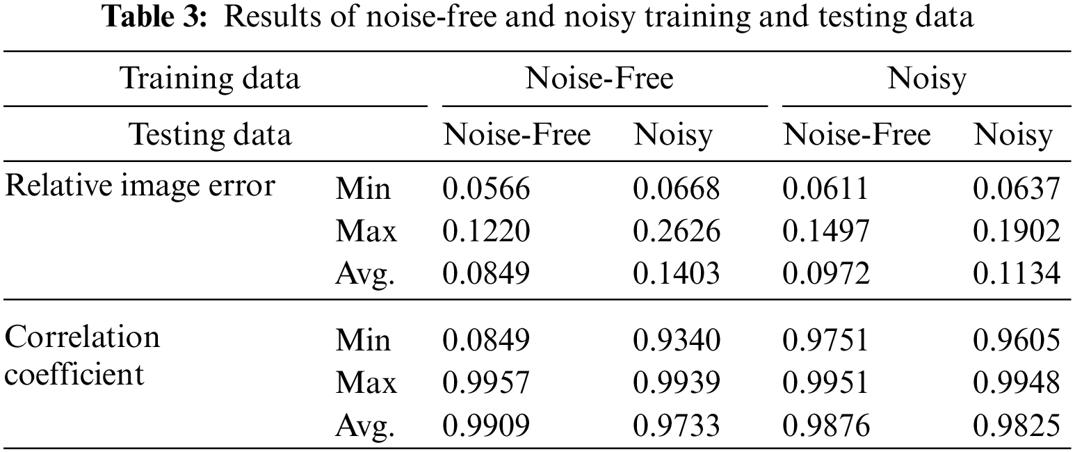
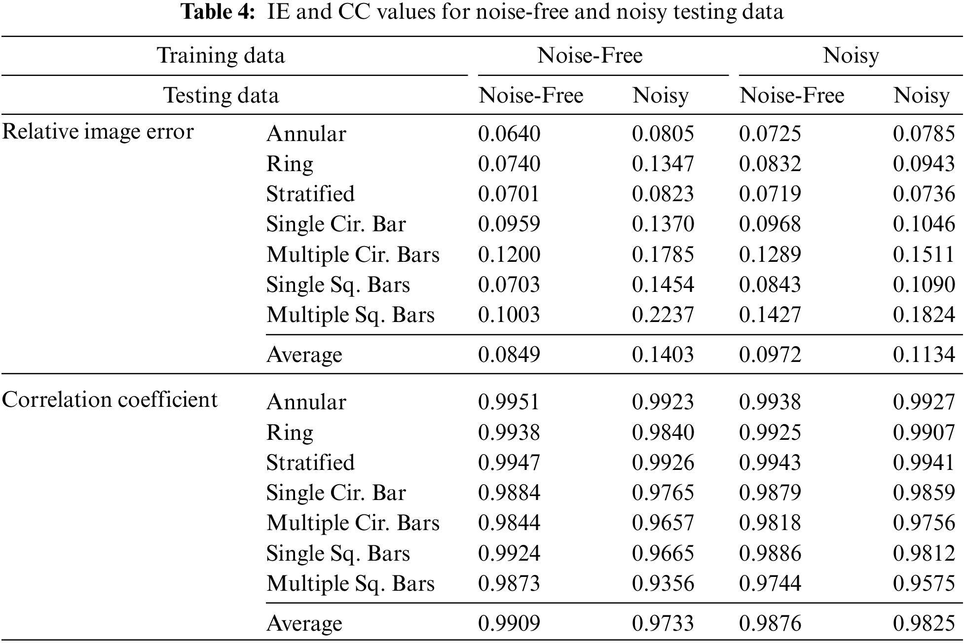
According to the values of the average relative IE and CC listed in Tab. 3 and Tab. 4, the trained ECT_ResAE model with noise-free data achieves better image reconstruction on the noise-free testing data compared with the other noisy data. Moreover, the trained model with the noisy data performs a little bit worse than those of free-noise training data but still substantial.
5.4 Testing with Phantoms not in the ECT Dataset
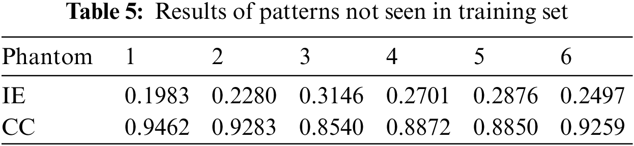
Capacitance measurements obtained from new two-phase flow models not seen in the training data set are applied to test the scalability capacity of the ECT_ResAE model. Six different materials distributions, named from 1 to 6, shown in first column of Fig. 11 are generated and inputted to the trained ECT_ResAE model without noise.
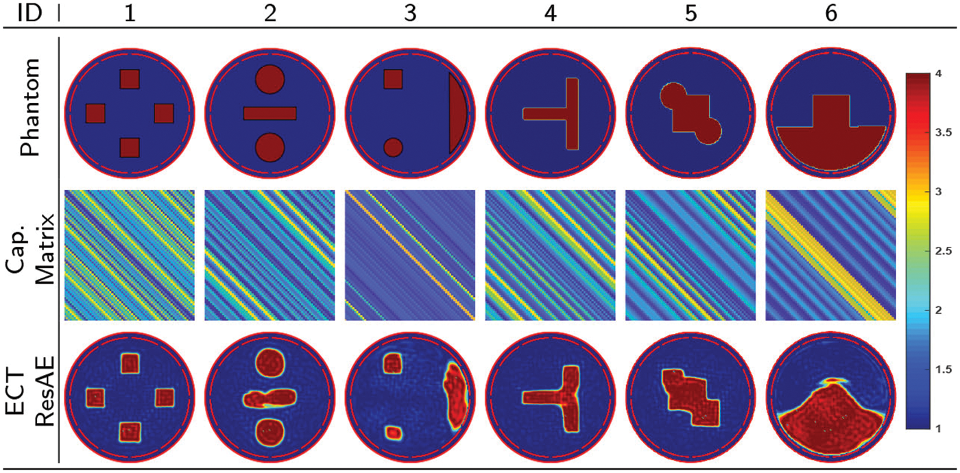
Figure 11: Reconstructed image of patterns not in training set
In the third column of the Fig. 11, the images reconstructed by the model ECT_ResAE are presented, and their corresponding relative IE and CC are listed in Tab. 5. However, there are not any mix between different types of the flow patterns as phantoms 2 3 in the training set, nor any four-square bars, the ECT_ResAE still can recognize its real patterns with high quality results. Although, the ECT suffers from the inhomogeneous sensitivity map problem across its cross-sectional sensing domain, the reconstructed image of the phantom number 5, 6 proves the ability of the ECT_ResAE method reconstructing phantoms located in the low and high sensitivity areas of the ECT sensor. The results are acceptable, although the reconstructed result is not quite sharp.
5.5 Testing with Real Experimental Data
The scalability of the ECT_ResAE model is also tested using data obtained from experiments. The measured capacitance vectors from three real phantoms representing the two-phase flow are applied as testing input for the trained ECT_ResAE model without noise. The capacitance measurements are collected using system developed by Tech4Imaging [49] called digital Electrical Capacitance Volume Tomography (ECVT). This system has 36 channels, works on a capacitance sensor of 12 electrodes, and it can generate 120 images/s. Static phantoms were placed in the imaging area with radius 63 mm. Two plastic rods (r = 20 mm) are placed inside the imaging area to simulate the bubble flow, whereas the imaging area is split into two section to experiment the stratified flow by placing a plastic plate in the middle, and filling one section with plastic particles (ε = 4). The annular flow is simulated by filling plastic particles around a circular plastic plate centered inside the imaging area.
The real phantoms are shown in the first column of Fig. 12, the second column shows the modulated capacitance matrix, while other columns contain the reconstructed images from LBP, iterative Tikhonov, CNN, LSTM-IR, and ECT_ResAE algorithms. Visually from the results, the ECT_ResAE model can reconstruct high accurate images with sharp edges between the empty and filled sectors compared with the other algorithms. Also, it is clear that the artifacts are few in the ECT_ResAE reconstructed two rods, and annular flows.
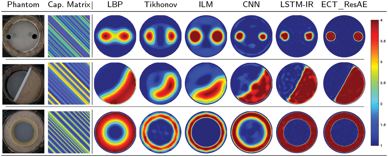
Figure 12: Experimental setup and reconstructed patterns
A new residual autoencoder deep neural model for reconstructing ECT images is proposed in this paper. A large-scale ECT simulation dataset has been created with 320k samples to train, validate, and test the proposed ECT_ResAE model. Besides, the model performance and its feasibility have been assessed by using contaminated data with noise, unseen flow patterns during training phase, and real experimental data. Results from different experiments prove that the proposed ECT_ResAE model has high performance in both visual effect and quantitative evaluation measures compared with the traditional and DNN ECT image reconstruction algorithms. For the online imaging, the ECT_ResAE model can reconstruct accurate ECT images as fast as the LBP algorithm. The overall generalization capability of the model is high where it achieved an average CC of more than 99%, and an average IE around 8.5%. Applying DNN models for reconstructing ECT images mainly depends on the training dataset and the richness of this dataset with different types of flow patterns having many features. Therefore, in our future work, we will build a new dataset including flow patterns with permittivity values which changes gradually, and we plan to train and test our proposed deep model by this dataset.
Acknowledgement: The authors would like to thank the Deanship of Scientific Research at Umm Al-Qura University for supporting this work by Grant Code: (22UQU4310447DSR02).
Funding Statement: The authors would like to thank the Deanship of Scientific Research at Umm Al-Qura University for supporting this work by Grant Code: (22UQU4310447DSR02).
Conflicts of Interest: The authors declare that they have no conflicts of interest to report regarding the present study.
References
1. Q. Guo, X. Li, B. Hou, G. Mariethoz, M. Ye et al., “A novel image reconstruction strategy for ECT: Combining two algorithms with a graph cut method,” IEEE Transactions on Instrumentation and Measurement, vol. 69, no. 3, pp. 804–814, 2020. [Google Scholar]
2. D. Yang, B. Zhou, C. Xu and S. Wang, “Thick-wall electrical capacitance tomography and its application in dense-phase pneumatic conveying under high pressure,” IET Image Processing, vol. 5, no. 5, pp. 513, 2011. [Online]. Available: https://digital-library.theiet.org/content/journals/10.1049/iet-ipr.2009.0209. [Google Scholar]
3. H. Guo, S. Liu, H. Cheng, S. Sun, J. Ding et al., “Iterative computational imaging method for flow pattern reconstruction based on electrical capacitance tomography,” Chemical Engineering Science, vol. 214, pp. 115432, 2020. [Google Scholar]
4. W. Q. Yang and L. Peng, “Image reconstruction algorithms for electrical capacitance tomography,” Measurement Science and Technology, vol. 14, no. 1, pp. R1–R13, 2003. [Google Scholar]
5. J. C. Gamio and C. Ortiz-Aleman, “An interpretation of the linear backprojection algorithm used in capacitance tomography,” in Proc. of 3rd WCIPT, Banff, Canad, pp. 427–432, 2003. [Google Scholar]
6. M. Vauhkonen, D. Vadâsz, P. A. Karjalainen, E. Somersalo and J. P. Kaipio, “Tikhonov regularization and prior information in electrical impedance tomography,” IEEE Transactions on Medical Imaging, vol. 17, no. 2, pp. 285–293, 1998. [Google Scholar]
7. Y. Li and W. Yang, “Image reconstruction by nonlinear landweber iteration for complicated distributions,” Measurement Science and Technology, vol. 19, no. 9, pp. 094014, 2008. [Google Scholar]
8. F. Li, J. Abascal, M. Desco and M. Soleimani, “Total variation regularization with split bregman-based method in magnetic induction tomography using experimental data,” IEEE Sensors Journal, vol. 17, no. 4, pp. 976–985, 2017. [Google Scholar]
9. W. F. Fang, “A nonlinear image reconstruction algorithm for electrical capacitance tomography,” Measurement Science and Technology, vol. 15, no. 10, pp. 21–24, 2004. [Google Scholar]
10. W. Deabes and K. E. Bouazza, “Efficient image reconstruction algorithm for ECT system using local ensemble transform 16alman filter,” IEEE Access, vol. 9, pp. 12779–12790, 2021. [Google Scholar]
11. M. Lopez de Prado, Advances in Financial Machine Learning. John Wiley and Sons, Hoboken, New Jersey, 2018. [Google Scholar]
12. H. Lee, R. Grosse, R. Ranganath and A. Y. Ng, “Convolutional deep belief networks for scalable unsupervised learning of hierarchical representations,” in Proc. of the 26th Annual Int. Conf. on Machine Learning, Montreal, Canada, pp. 609–616, 2009. [Google Scholar]
13. G. E. Hinton, S. Osindero and Y. Teh, “A Fast-learning algorithm for deep belief nets,” Neural Computation, vol. 18, no. 7, pp. 1527–1554, 2006. [Google Scholar]
14. Y. LeCun, Y. Bengio and G. Hinton, “Deep learning,” Nature, vol. 521, no. 7553, pp. 436–444, 2015. [Google Scholar]
15. H. Zhu, J. Sun, J. Long, W. Tian and S. Sun, “Deep image refinement method by hybrid training with images of varied quality in electrical capacitance tomography,” IEEE Sensors Journal, vol. 21, no. 5, pp. 6342–6355, 2021. [Google Scholar]
16. Z. Xu, F. Wu, L. Zhu and Y. Li, “LSTM model based on multi-feature extractor to detect flow pattern change characteristics and parameter measurement,” IEEE Sensors Journal, vol. 21, no. 3, pp. 3713–3721, 2021. [Google Scholar]
17. J. Zheng and L. Peng, “A deep learning compensated back projection for image reconstruction of electrical capacitance tomography,” IEEE Sensors Journal, vol. 20, no. 9, pp. 4879–4890, 2020. [Google Scholar]
18. G. Sulong and A. Mohammedali, “Human activities recognition via features extraction from skeleton,” Journal of Theoretical and Applied Information Technology, vol. 68, no. 3, pp. 645–650, 2014. [Google Scholar]
19. J. Zheng, J. Li, Y. Li and L. Peng, “A benchmark dataset and deep learning-based image reconstruction for electrical capacitance tomography,” in Sensors (Basel, Switzerland) MDPI, vol. 18, no. 11, 2018. [Google Scholar]
20. W. Deabes, A. Sheta, K. E. Bouazza and M. Abdelrahman, “Application of electrical capacitance tomography for imaging conductive materials in industrial processes,” Journal of Sensors, vol. 2019, no. ii, pp. 1–22, 2019. [Online]. Available: https://www.hindawi.com/journals/js/2019/4208349/. [Google Scholar]
21. W. Deabes and H. H. Amin, “Image reconstruction algorithm based on pso-tuned fuzzy inference system for electrical capacitance tomography,” IEEE Access, vol. 8, pp. 191875–191887, 2020. [Google Scholar]
22. S. Antholzer, M. Haltmeier, and J. Schwab, “Deep learning for photoacoustic tomography from sparse data,” Inverse Problems in Science and Engineering, vol. 25, no. 4, pp. 987–1005, 2017. [Google Scholar]
23. A. Hauptmann, F. Lucka, M. Betcke, N. Huynh, J. Adler et al., “Model-based learning for accelerated, limited-view 3-d photoacoustic tomography,” IEEE Transactions on Medical Imaging, vol. 37, no. 6, pp. 1382–1393, 2018. [Google Scholar]
24. C. Tan, S. Lv, F. Dong and M. Takei, “Image reconstruction based on convolutional neural network for electrical resistance tomography,” IEEE Sensors Journal, vol. 19, no. 1, pp. 196–204, 2019. [Google Scholar]
25. K. H. Jin, M. T. McCann, E. Froustey and M. Unser, “Deep convolutional neural network for inverse problems in imaging,” IEEE Transactions on Image Processing, vol. 26, no. 9, pp. 4509–4522, 2017. [Google Scholar]
26. E. Kang, J. Min and J. Ye, “A deep convolutional neural network using directional wavelets for low-dose X-ray ct reconstruction,” Medical Physics, vol. 44, no. 10, pp. e360–e375, 2017. [Google Scholar]
27. C. M. Sandino, N. Dixit, J. Y. Cheng and S. S. Vasanawala, “Deep convolutional neural networks for accelerated dynamic magnetic resonance imaging,” in 31st Conf. on Neural Information Processing Systems (NIPS 2017), Long Beach, CA, USA, pp. 1–4, 2017. [Google Scholar]
28. D. Xie, L. Zhang and L. Bai, “Deep learning in visual computing and signal processing,” Applied Computational Intelligence and Soft Computing, vol. 2017, pp. 1–13, 2017. [Google Scholar]
29. J. Zheng, H. Ma and L. Peng, “A CNN-based image reconstruction for electrical capacitance tomography,” in Proc. of IEEE Int. Conf. on Imaging Systems and Techniques, IST, IEEE, Abu Dhabi, UAE, pp. 1–6, 2019. [Google Scholar]
30. W. Lili, L. Xiao, C. Deyun, Y. Hailu and C. Wang, “ECT image reconstruction algorithm based on multiscale dual-channel convolutional neural network,” Complexity, vol. 2020, pp. 1–12, 2020. [Google Scholar]
31. Z. Cao, L. Xu, W. Fan and H. Wang, “Electrical capacitance tomography with a non-circular sensor using the Dbar method,” Meas. Sci. Technol, vol. 21, pp. 1–6, 2009. [Google Scholar]
32. J. Zheng and L. Peng, “An autoencoder-based image reconstruction for electrical capacitance tomography,” IEEE Sensors Journal, vol. 18, no. 13, pp. 5464–5474, 2018. [Google Scholar]
33. J. Li, X. Yang, Y. Wang and R. Pan, “An image reconstruction algorithm based on RBF neural network for electrical capacitance tomography,” in 2012 Sixth Int. Conf. on Electromagnetic Field Problems and Applications, Dalian, China, no. 2, pp. 1–4, 2012. [Google Scholar]
34. W. Deabes, A. Sheta and M. Braik, “ECT-LSTM-RNN: An electrical capacitance tomography model-based long short-term memory recurrent neural networks for conductive materials,” IEEE Access, vol. 9, pp. 76325–76339, 2021. [Google Scholar]
35. W. Deabes and K. M. J. Khayyat, “Image reconstruction in electrical capacitance tomography based on deep neural networks,” IEEE Sensors Journal, vol. 21, no. 22, pp. 25818–25830, 2021. [Google Scholar]
36. P. Isola, J. Y. Zhu, T. Zhou and A. A. Efros, “Image-to-image translation with conditional adversarial networks,” in Proc. of the IEEE Conf. on Computer Vision and Pattern Recognition, Honolulu, HI, USA, pp. 1125–1134, 2017. [Google Scholar]
37. K. Zeng, J. Yu, R. Wang, C. Li and D. Tao, “Coupled deep autoencoder for single image super-resolution,” IEEE Transactions on Cybernetics, vol. 47, no. 1, pp. 27–37, 2015. [Google Scholar]
38. J. Xie, L. Xu and E. Chen, “Image denoising and inpainting with deep neural networks,” Advances in Neural Information Processing Systems, vol. 25, pp. 341–349, 2012. [Google Scholar]
39. R. Qian, R. T. Tan, W. Yang, J. Su and J. Liu, “Attentive generative adversarial network for raindrop removal from a single image,” in Proc. of the IEEE Conf. on Computer Vision and Pattern Recognition, Salt Lake City, UT, USA, pp. 2482–2491, 2018. [Google Scholar]
40. K. He, X. Zhang, S. Ren and J. Sun, “Deep residual learning for image recognition,” in Proc. of the IEEE Conf. on Computer Vision and Pattern Recognition, Las Vegas, NV, USA, pp. 770–778, 2016. [Google Scholar]
41. M. Feng, H. Lu and Y. Yu, “Residual learning for salient object detection,” IEEE Transactions on Image Processing, vol. 29, pp. 4696–4708, 2020. [Google Scholar]
42. T. Li, H. Song, K. Zhang and Q. Liu, “Recurrent reverse attention guided residual learning for saliency object detection,” Neurocomputing, vol. 389, pp. 170–178, 2020. [Google Scholar]
43. W. A. Deabes and M. A. Abdelrahman, “A nonlinear fuzzy assisted image reconstruction algorithm for electrical capacitance tomography,” ISA Transactions, vol. 49, no. 1, pp. 10–18, 2010. [Google Scholar]
44. X. Wang, K. Yu, S. Wu, J. Gu, Y. Liu et al., “Esrgan: Enhanced super-resolution generative adversarial networks,” in Proc. of the European Conf. on Computer Vision (ECCV) Workshops, Munich, Germany, 2018. [Google Scholar]
45. J. Man and G. Sun, “A residual learning-based network intrusion detection system,” Security and Communication Networks, vol. 2021, pp. 1–9, 2021. [Google Scholar]
46. Z. Cui, Q. Wang, Q. Xue, W. Fan, L. Zhang et al., “A review on image reconstruction algorithms for electrical capacitance/resistance tomography,” Sensor Review, vol. 36, no. 4, pp. 429–445, 2016. [Google Scholar]
47. M. Abadi, A. Agarwal, P. Barham, E. Brevdo, Z. Chen et al., “TensorFlow: Large-scale machine learning on heterogeneous systems,” arXiv, preprint arXiv:1603.04467, 2016. [Google Scholar]
48. F. Chollet et al. “Keras,” GitHub, 2015. [Online]. Available: https://github.com/keras-team/keras. [Google Scholar]
49. Tech4imaging electrical capacitance volume tomography, Ohio, USA. 2020. Available: https://www.tech4imaging.com/. [Google Scholar]
 | This work is licensed under a Creative Commons Attribution 4.0 International License, which permits unrestricted use, distribution, and reproduction in any medium, provided the original work is properly cited. |