Computers, Materials & Continua DOI:10.32604/cmc.2022.030803
Article

Deep Reinforcement Learning-Based Job Shop Scheduling of Smart Manufacturing

Eman K. Elsayed1, Asmaa K. Elsayed2,* and Kamal A. Eldahshan3

1School of Computers Science, Canadian International College (CIC). Department of Mathematics, Faculty of Science (Girls), AL-Azhar University, Cairo, 11511, Egypt
2Department of Mathematics, Faculty of Science(Girls), AL-Azhar University, Cairo, 11511, Egypt
3Department of Mathematics, Faculty of Science, AL-Azhar University, Cairo, 11511, Egypt
*Corresponding Author: Asmaa K. Elsayed. Email: asmaa_sciences90@yahoo.com
Received: 02 April 2022; Accepted: 19 May 2022

Abstract: Industry 4.0 production environments and smart manufacturing systems integrate both the physical and decision-making aspects of manufacturing operations into autonomous and decentralized systems. One of the key aspects of these systems is a production planning, specifically, Scheduling operations on the machines. To cope with this problem, this paper proposed a Deep Reinforcement Learning with an Actor-Critic algorithm (DRLAC). We model the Job-Shop Scheduling Problem (JSSP) as a Markov Decision Process (MDP), represent the state of a JSSP as simple Graph Isomorphism Networks (GIN) to extract nodes features during scheduling, and derive the policy of optimal scheduling which guides the included node features to the best next action of schedule. In addition, we adopt the Actor-Critic (AC) network’s training algorithm-based reinforcement learning for achieving the optimal policy of the scheduling. To prove the proposed model’s effectiveness, first, we will present a case study that illustrated a conflict between two job scheduling, secondly, we will apply the proposed model to a known benchmark dataset and compare the results with the traditional scheduling methods and trending approaches. The numerical results indicate that the proposed model can be adaptive with real-time production scheduling, where the average percentage deviation (APD) of our model achieved values between 0.009 and 0.21 compared with heuristic methods and values between 0.014 and 0.18 compared with other trending approaches.

Keywords: Reinforcement learning; job shop scheduling; graphical isomorphism network; actor-critic networks

1  Introduction

Along with the fourth industrial revolution, a Smart Factory [1,2] provides flexible and adaptive production processes that can solve problems appearing in production with dynamic and rapidly changeable conditions; therefore, it is a need for flexibility in the job scheduling system that can achieve balance scheduling efficiency and its costs. From recently reviewed, there are fourteen classes of JSSP classified as [Deterministic JSSP, static JSSP, dynamic JSSP, flexible JSSP, cyclic JSSP, periodic JSSP, pre-emptive JSSP, just-in-time JSSP, no-wait JSSP, large-scale JSSP, re-entrant JSSP, assembly JSSP, stochastic JSSP, and fuzzy JSSP] have been identified in [3]; based on their main characteristics as Job arrival process, inventory policy, duration time processing, and job attributes. In our research, we regard the problem as the flexible JSSP of a manufacturing system.

To solve JSSP problems of different scales, several efficient algorithms have been proposed by researchers to improve various parameters of JSSP. Exact arithmetic-based methods using an integer programming formula are introduced by [4–8] but the time is usually not acceptable when large-scale problems are encountered because the solution space is larger will lead to computational complexity.

Heuristics algorithms are capable of real-time decision-making introduced in [9,10] and it only depends on the limited information, which leads to the instability of the performance of the algorithm. The meta-heuristic algorithms that are problem-independent and a class of algorithmic frameworks that are proposed in [11–14] and the performance of these algorisms depends on the control of parameters, in addition, when the size of the problem increases, there is a slowdown in the performance of the algorithm. One of the recent trends that solve the scheduling problem is Hadoop Yarn [15], it is a framework, that provides a management scheduling for big data in a distributed environment, but it is only suitable for large data volume. With the common technology, different tools for optimization, such as data science, the Internet of Things (IOTs) [16], and artificial intelligence AI fields create new opportunities in production control. Many studies apply the reinforcement learning approach to model routing and scheduling optimization problems such as [17–24], which performed better than traditional algorithms on some complex combinatorial optimization problems. Researchers in [25–27] introduced Graph Neural Networks (GNN) and GIN to take advantage of the graph representation and solve graph-based optimization problems; they are an innovative combination of aggregative optimization and deep learning.

In this paper, we propose a framework to construct the scheduling policy for JSSPs using the DRL mechanism, it can learn to choose appropriate actions to achieve its goals through system environment interactions and respond to reward receipts based on the impact of each action. First, we formulate the scheduling of a JSSP as a sequential decision-making problem in an MDP concept, and then we represent the state of a JSSP as a graph representation, consisting of operations that represent nodes and constraints that represent edges. Next, we use GIN [28] to learn node features and derive a scheduling policy that defines the included node features to get optimal scheduling. Thus, when focusing on JSSPs, the output of the neural network directly reflects the priority value of the appropriate action to act according to the current state. In addition, we introduced the actor-critic network algorithm into the job-shop scheduling with a good performance and low complexity for the training and learning agent. For more explanation, we illustrate our proposed framework in Fig. 1.

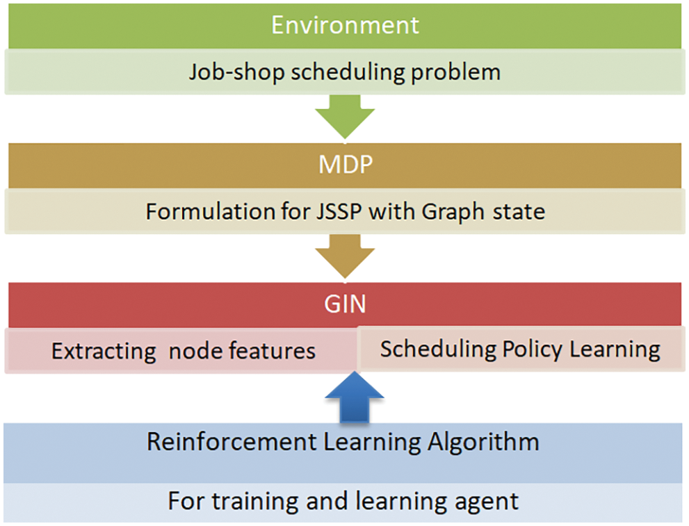
Figure 1: Explanation of the proposed framework

We organized the rest of the paper as follows: Section 2 Explains the methods used in this research. Section 3 introduced the DRLAC for job-shop scheduling with the proposed architecture. Section 4. Introduced the experiments in two parts, using case study and using benchmarks data set then result-analysis stated, finally the Conclusions and Future Research presented in Section 5.

2  Methodology

2.1 Job Shop Scheduling Problem (JSSP) Description

JSSP is a type of scheduling problem that aims to define optimal sequential assignments of machines to multiple jobs consisting of a sequence of operations while maintaining problem constraints (such as processing precedence and machine sharing).

When a request is received for n jobs defined as J = {j1, j2,.., jn}, it must specify how to allocate it to the assigned number of machines and create an appropriate production schedule.

Each machine can produce kinds of product with different efficiency, defined as M = {m1, m2,…, mm} and each job can be directed through m machines in a predetermined order.

The processing of a job on a machine is called an operation; each operation can be processed on one or more suitable machines with different processing times. The operation can be denoted by Oij and the set of operations can be formulated in the form of O = {Oij | i ∈ [1, n], j ∈ [1, m]}. For an operation, Oijof job i on machine m, the processing time of operation can be denoted by Pij where (Pij > 0), and the total completion time for a set of operations is Cij (Oij ∈O). Thus, the main goal of the problem is to minimize C.

Therefore, the job shop-scheduling problem is regarded as a sequential decision problem for assigning jobs to specific machines. We explained the constraints of JSSP as the following:

•   As soon as the process of a job can begin at any time, the required machine becomes available.

•   Each job must pass through a series of pre-defined operations, where operation cannot be started until the previous one is complete, (i.e., processing Oij cannot begin the processing on a machine until Oij−1 has been completed).

•   One or more machines must process each operation completely.

•   When assigning jobs to machines, it is necessary to consider whether the machines have operations that can be processed by a machine at this time.

•   If there are multiple optional choose operation sets, the machine can select one of them for processing. Otherwise, it needs to wait for the arrival of the next operation processing completion event.

2.2 Disjunctive Graph Representation for JSSP

The solution approach applied in this paper is based on a graph, and represents JSSP as G = (N, C, D) where:

•   N is the set of nodes representing the processes and N = O U {O0} U {OT+1}] where {O0} and {OT+1} are the special dummy operations of the start and end of the node. T is the total number of operations that T = n × m,

•   C is a set of directed-lines (conjunctions) that connect approved operations of the same job,

•   D is a set of undirected-lines (disjunctions), which connect operations performed on the same machine.

To illustrate job-scheduling problems, we assume the JSSP problem as n/m/G/Cmax JSSP, the idea of the proposed model is to start a set of nodes iteratively, Which moves in a common environment consisting of all operations in JSSP. We build a graphical representation of the optimization problem as Fig. 2, which represents the number of nodes representing all Oij, where O11 to O1j for the first job and O21 to O2j for the second job, etc., two dummy nodes (S, E) for the start and end of routing of total operations. The directional edges connect nodes that indicate the precedence constraints.

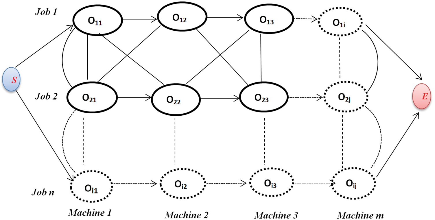
Figure 2: JSSP graphical representation for size problem nxm

Later, in this paper, we can potentially deal with complex environments with dynamics and uncertainty conflicting such as job arriving, by adding or removing certain nodes and/or lines from the disjunctive graphs.

We represent the state of JSSP using a disjunctive graph like the following:

•   Nodes are represented as operations,

•   Conjunctive edges are represented as precedence constraints between two nodes,

•   Disjunctive edges are represented as machine-sharing constraints between two operations.

2.3 Markov Decision Process Formulations for JSSP

Since the next job processing state only changes based on the present state, we can model the job shop-scheduling problem as an MDP. Therefore, we will consider the decisions of dispatching as actions of changing the graph, and we formulate the MDP model as the following:

State. The state noted as st at decision step t is a disjunctive graph DGt = (O, C ∪ ADt, RDt) representing the current status of the solution; where ADt ⊆ D includes all the directed disjunctive lines which have been assigned a direction till step t and RDt ⊆ D includes the remaining ones. The initial state So is the disjunctive graph that represents the original instance of the problem, and the terminal state sT is a complete solution where RDT = ∅, i.e., all disjunctive lines have been assigned a direction.

For each node O ∈ N, we record two features, the operations that they are scheduling in st, and the completion lower bound (LB) duration of the estimated time of operation completion in st, we regard the (LB) as exactly its minimum completion time. Towards the unscheduled operation of job Ji, we calculate this lower bound as Eq. (1) recursively by only considering the precedence restrictions from its predecessor, i.e., Oi, j−1 → Oij, and Eq. (2) where Oij is the first operation of Ji and riis the release time of Ji.

LB(Oij,st)=LB(Oij−1,st)+Pij(1)

LB(Oij,st)=ri+Pij(2)

Action. An action at ∈ At is an appropriate operation at decision step t. when each job can have at most one operation at t, the maximum size of action procedure space is |J|, which depends on the instance performed. During processing, |At| will be smaller as more jobs are completed.

State-transition. Once determining an operation to dispatch next, we first find the closest possible period to allocate to the desired machine. Next, we update the trends of that machine’s disjunctive lines based on the time relationships and create a new disjunctive graph as the new state st+1.

Reward. For each action the agent performs, the environment will return the corresponding reward. Since we used the reward to evaluate the action performed, the setting of it directly affects the change of the agent strategy.

Policy. For state St, a stochastic policy denoted by π (at|st) results in distribution over the actions in At. To obtain the optimal policy to solve the JSSP it is very important to set appropriate rewards.

Our problem environment will feedback a corresponding reward for each agent action, so the paper will propose to set the reward in the job shop scheduling process to be related to machine functions, which means that the optioned makespan will be a function of cumulative rewards. This leads to obtaining the optimal policy to solve our problem and get an optimal or near-optimal solution (min makespan); we formulate the reward as the minim of the makespan Cmax, computed as {min Cmax (Oij, st)}.

2.4 Graph Isomorphism Network (GIN)

GIN is one such example among many maximally powerful GNNs, while being simple [29], it is based on graph operations that include training a neural network for various graph-related tasks, and it seems to be effective on social datasets [30]. Two multi-layer of GINS are used to encode the features constraint and processing time characteristics of the flow shop problem scheduling, they can efficiently aggregate node features and other neighbor features to get for each node the contextual representation [27].

The disjunctive graph based on the MDP formula provides an overview of the scheduling states containing numerical and structural information such as processing time of operation, each processing order of the machine, and precedence constraints. The efficient transmission is viable when extracting all the state information from disjunctive graphs. This prompts us to select the stochastic policy π (at |st) as the GIN with θ trainable parameter, i.e., πθ (at |st) enables learning strong dispatching rules.

Fig. 3 is an example that explains the difference between the deterministic policy concept and the stochastic policy concept intended in our research to obtain scheduling optimization.

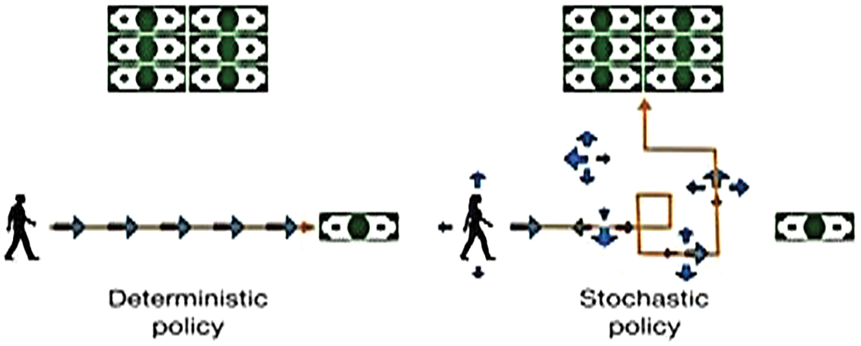
Figure 3: The concept of deterministic and stochastic policy

Given a graph G = (V, E), GIN performs K iterations of update expressed as Eq. (3):

hkv=MLPkθk((1+ϵk).hk−1v+∑uϵN(v)hk−1u(3)

where hkv is node v representation of iteration k, h0v indicated his initial features for the input, MLPkθk is a Multiable-Layer Perceptron for iteration k with parameter θk, and N(v) is the v neighborhood.

After updates iterations K, the global representation of the entire graph can be obtained using the aggregate function L which takes as input information for all nodes and outputs the dimensional vector hg formed in Eq.(4).

hg=L({hvk:vϵV})=1/|V|∑vεV⁡hvk(4)

The disjunctive Gt graph associated with each state st is the mixed graph with directed-lines, which describe the critical characteristics such as the operation sequences on machines and the precedence constraints, therefore, we need to generalize the GIN for supporting disjunctive graphs. When adding incoming neighbor u of v, then the neighborhood of node v in Eq. (3) can be defined as N (v) = {u| (u, v) ∈ E (GD) t}, where GD is a directed graph i.e., NV contains all incoming neighbors of v.

3  DRL Based Actor-Critic for Job-Shop Scheduling

3.1 Model Description

In reinforcement learning methods, comparing value-based methods, policy-based methods are more suitable for continuous state and action space problems such as JSSP. This is useful in our problem environment because the action space is continuous and dynamic and has a faster convergence. Reinforcement learning occurs when the agent interacts with its surrounded environment to perform actions and learn by a trial-error learning method.

As one of the policy-based methods, the actor-critic one of the RL training algorithms can obtain good performance by limiting the policy update to reduce parameter settings sensitivity. The Actor refers to the policy network πθ described in the previous section, it controls how the agent behaves by learning the optimal policy (policy-based). The critic vφ shares the GIN network with the actor and uses MLPkθk that takes the input of hG(st) to output a scalar to estimate the cumulative rewards at st, it evaluates the action by computing the value function (value-based).

To raise learning, we follow the principle of AC and update network parameters. For JSSP, DRL can implement real-time scheduling and adapt strategies based on the environment’s current state when dealing with problems. DRL aims to enable the agent to learn to take actions to maximize the cumulated reward from the process of interacting with the environment.

3.2 DRLAC Model Architecture

We present in Fig. 4 the DRLAC architecture of the job-shop scheduling based on the AC algorithm. There are two main parts to this architecture:

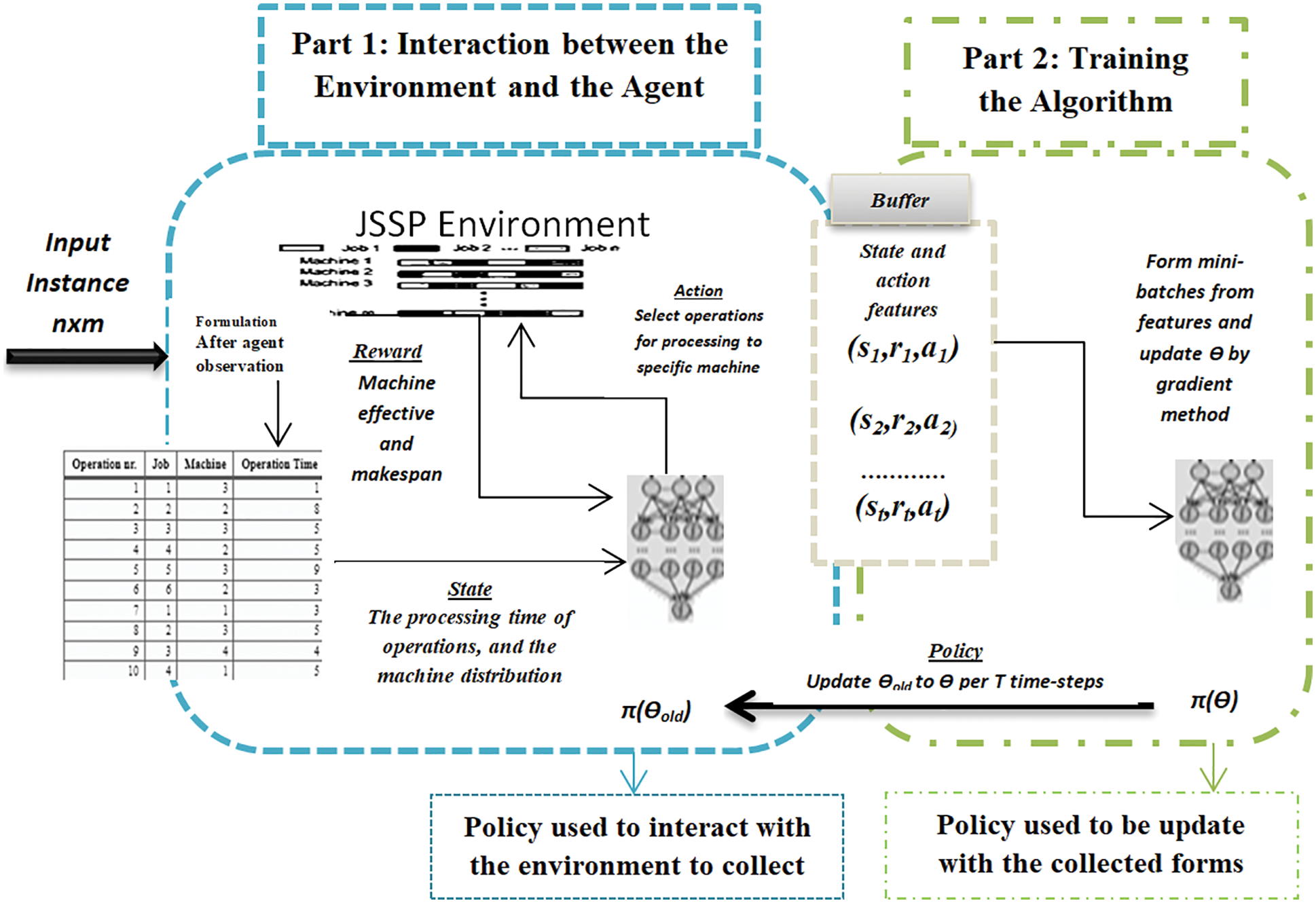
Figure 4: The architecture of DRLAC for job-shop scheduling

(1) The Interaction Part between the Agent and the Environment

We define the environment as a set of jobs with their assigned machines and their processing time. For the JSP environment, the agent needs to observe the information of the environment state at each moment, such as the processing status of jobs, the assigned machine matrix, and the processing time matrix, and then take action to select operations for appropriate machines to make jobs be processed in an orderly manner with the minimum of maximum completion time. To select an action at, we further process the extracted graph information hvk with an action selection network. In doing so, we expect to produce a probability distribution over action space from which at can be formed. The agent receives the reward function about the machine utilization after the action is executed and the environment gives makespan, then the next state of the environment is to run the next step for the system.

(2) The training part of the algorithm

This is the part of the agent policy update, where the buffer memory forms mini-batches to update πθ.The parameter θ is updated according to the stochastic gradient method to optimize the objective function L(θ) of the AC algorithm. In this way, the dynamic JSSP system based on AC is constructed. The agent interacts with the JSSP environment in a trial and error manner at the beginning of training. The agent can make real-time decisions on the job shop environment once it learns the optimal policy using the trained model, thus achieving real-time job shop scheduling. Moreover, when the agent faces an unknown environment state, it can make a good decision by updating the policy network in real-time, to achieve flexible scheduling.

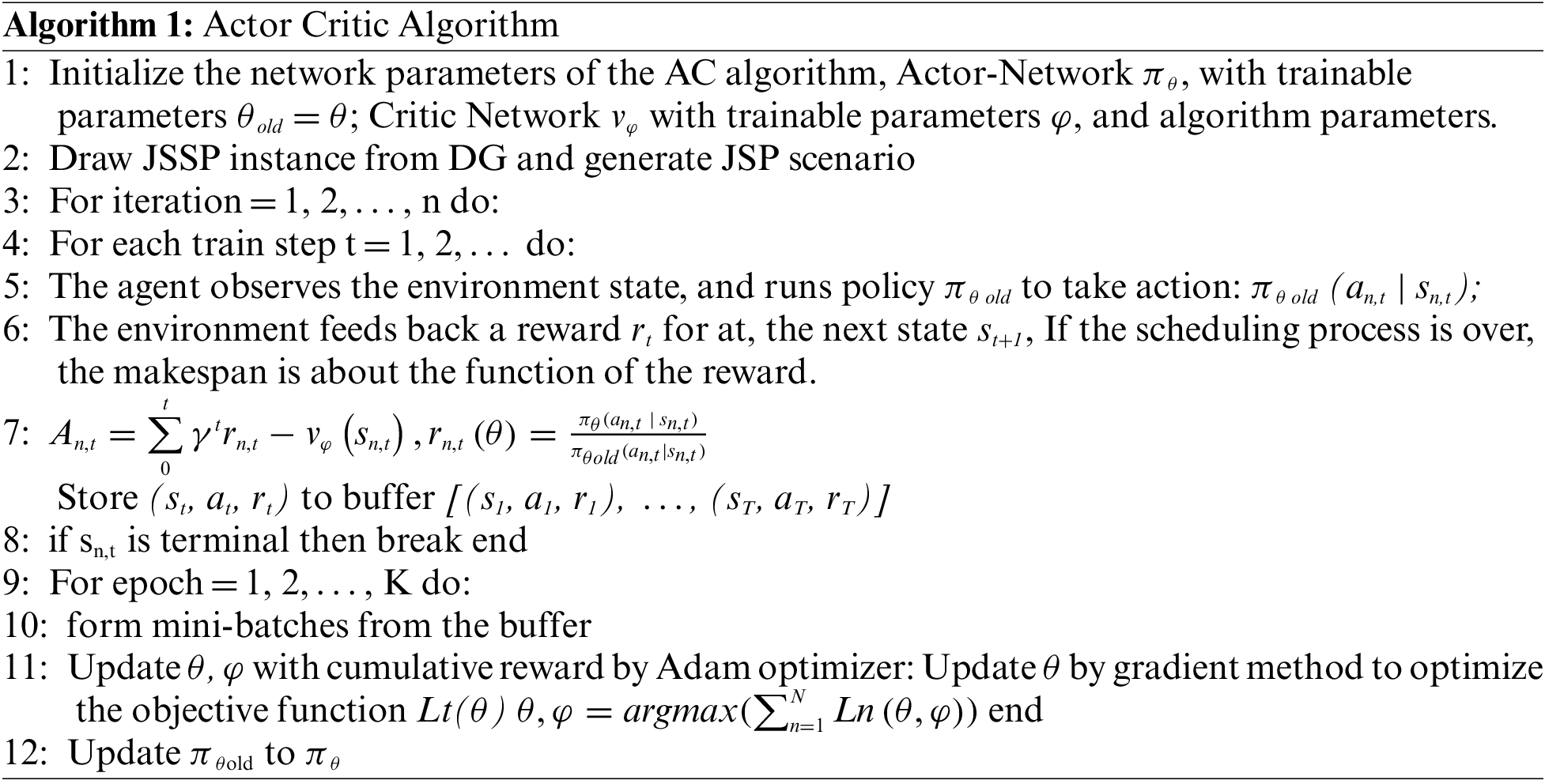
3.3 Pseudo-Code for the Proposed Algorithm

We adopt the Actor-Critic algorithm to train our agent and provide details of our algorithm in terms of pseudo-code, as shown in Algorithm 1; it provides pseudo-code for RL agent interacting with an environment with changing action sets.

4  Experimentally and Result Analysis

4.1 Configuration and Hyper-Parameters Setting

We used the settings that were previously used in our research and they performed well in [31], shown in Tab. 1, the results indicated that our proposed model has more effective to solve the problems with big data set that has more than 100 jobs and 100 machines.

In this research, we use the Adam optimizer for training the AC algorithm. Other parameters follow the default settings in PyTorch [26] and use the repository of its implementation [32] with python machine learning as Numpy (library used for working with arrays), Torch (provides a flexible N-dimensional array), Tensor(supports basic routines for indexing), TensorFlow (libraries used to create Ultimate Software’s Python-based, AI open-source generation and testing tool Agent or AgentX) and Gym (communicate between learning algorithms and environments). In addition to Microsoft Excel to store, analyze, and chart generating data. The hardware we use is a machine with an Intel Core i5 CPU and a single NVIDIA GeForce GPU with Windows 10 as an operating system.

The evaluation criterion in the experiment is the maximum completion time ‘makespan’ and our goal is to minimize it.

Compared to optimization strategies, Reinforcement learning allowed making moves with a negative reward. Therefore, we set the returned reward in our model as negative rewards. In general, we prefer to have negative returns for stability purposes. If you do back-propagation equations, you will see that yield affects gradients. Thus, we like to keep their values in a specific appropriate range, so if you increase or decrease all rewards (good and bad) equally, nothing will change.

4.2 Experimentally Using Case Study

4.2.1 Computational Results on Instances Before Conflicting in Job Scheduling

We suppose that a job instance for two jobs J1and J2 are scheduled simply performed in three machines M1, M2, and M3 distributed in Tab. 2, it illustrates that each job j has an associated processing time and is to be assigned to a single machine, and each machine can process at most one job at a time.

When modeling this instance as a disjunctive graph G = (J, E) and if {j, j′} ∈ E then jobs j and j′ are two conflicting jobs, and they must be assigned to different machines.

Each job has three operations, each operation o can assign to one machine sequentially and it has a processing time PT that it takes for performing on the machine. The minimum completion time takes to complete the scheduling process (makespan) is 47 UT.

Now to prove the NP-hard problem of job scheduling, we suppose an additional job J3 with an addition node has operations [o31, o32, o33] and needed to assign to machines [2, 3, 1] with processing time [20, 20, 10] sequentially. In a traditional dispatching algorithm such as FIIFO, the scheduling is solved by keeping track in a queue of the previous arrival job in front and the recent addition job at the back.

Fig. 5 illustrates the distribution of the additional job based on the First in First Out (FIFO) rule, that operation o31 begins to handle after the last operation o23 so the maximum completion time takes to complete the scheduling process is Cmax = 97 UT.

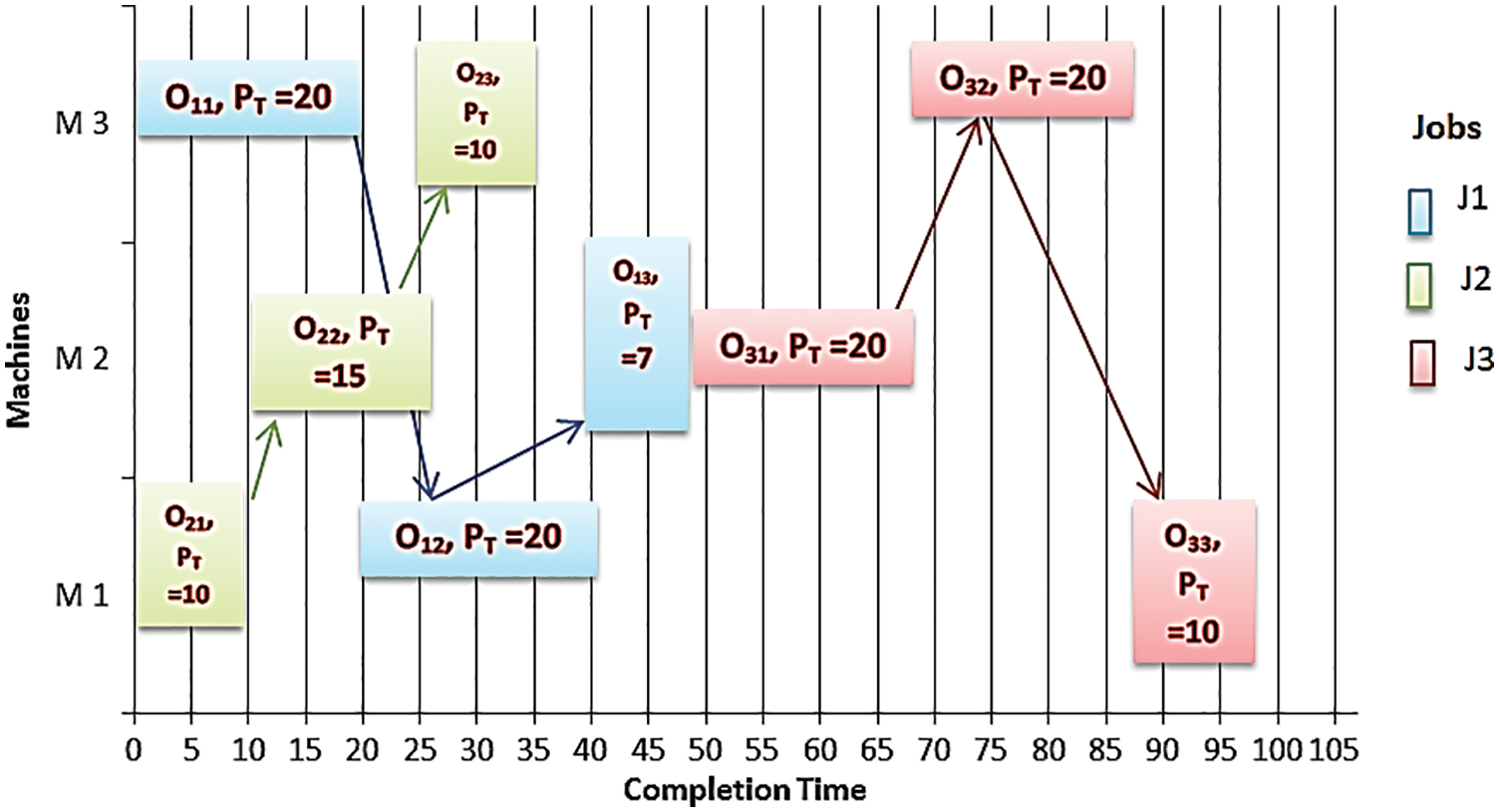
Figure 5: The scheduling of 3 × 3 instance-based FIFO algorithms with Cmax = 97

Fig. 6 illustrates the optimal scheduling of addition job distribution where the operation o31 is performed before o22 in machine two and operation o32 is performed before operation o23 in M3 based on the Longest Processing Time (LPT) rule with a less waiting time equal to 20 UT, and the maximum completion time taken is Cmax= 50 UT.

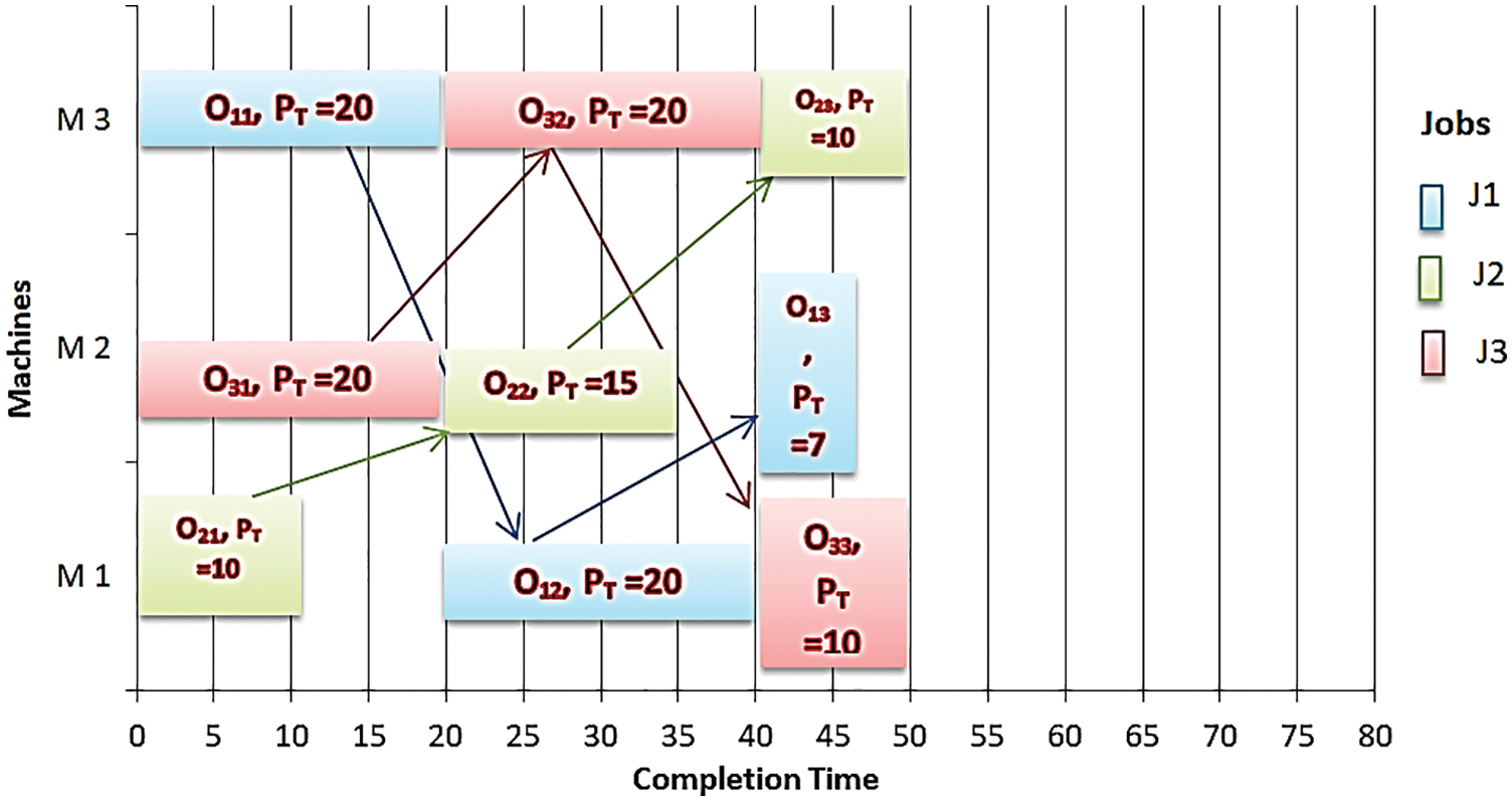
Figure 6: The optimal scheduling of 3 × 3 instance with Cmax = 50

4.2.2 Computational Results on Instances with Two Conflicting Jobs Scheduling

When we assume that the operations of two jobs have the same requirement for each machine, a conflict engenders between a subset of jobs, and the requirement of at least one machine exceeds its capacity.

We consider the previous instance of three jobs {J1, J2, J3} to be processed on three machines. Suppose that we have one rescheduling job 3 such that J3 operations [o31, o32, o33] needed to assign to machines [2, 1, 3] with processing time [20, 10, 20] sequentially. Hence, J1 and J3 are conflicting shown in Fig. 7, where the second operation o12 of J1 and the second operation o32 of J3 needed to be performed in machine one at the same time = 20 UT, which means the requirement of two jobs exceeds the machine one capacity at the same time. Therefore, this case requires a rescheduling.

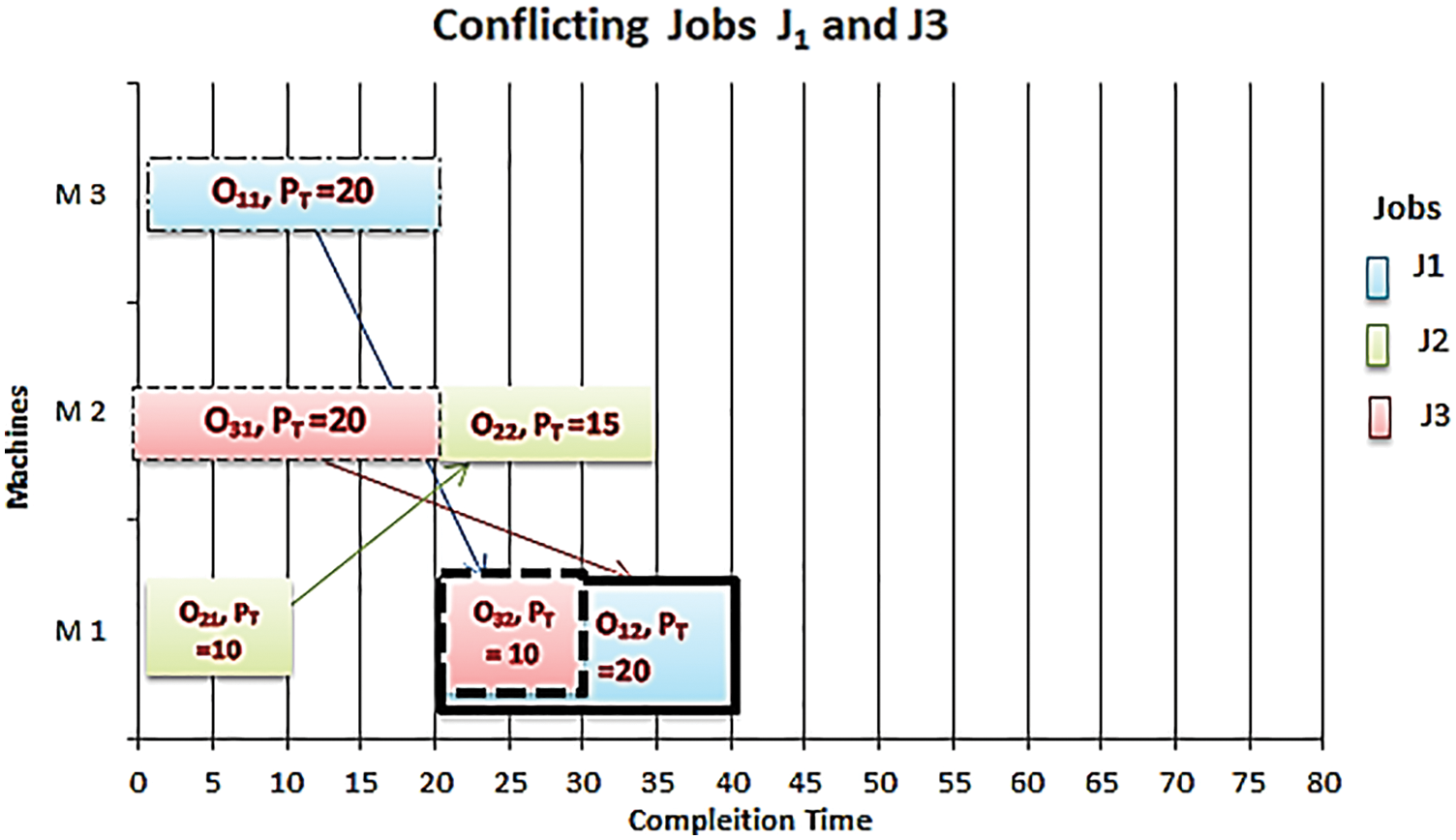
Figure 7: J1 and J3 are conflicting at machine M1

The first operation o31 of J3 was performed before o22 of J2 in machine two based on the LPT rule, this leads to the conflict between the two next operations of J1and J3, and the second operation of the two jobs needed to perform at the same machine and the same time.

The optimal solution of this instance can obtain different values of compilation time based on Remaining Processing Time RPT obtains Cmax = 70 or 65 and 60 UT with different job distribution in two cases shown in Figs. 8A, 8B. Based on FIFO Algorithm, the completion time of this instant case is equal to 97 UT as in the previous case shown in Fig. 4.

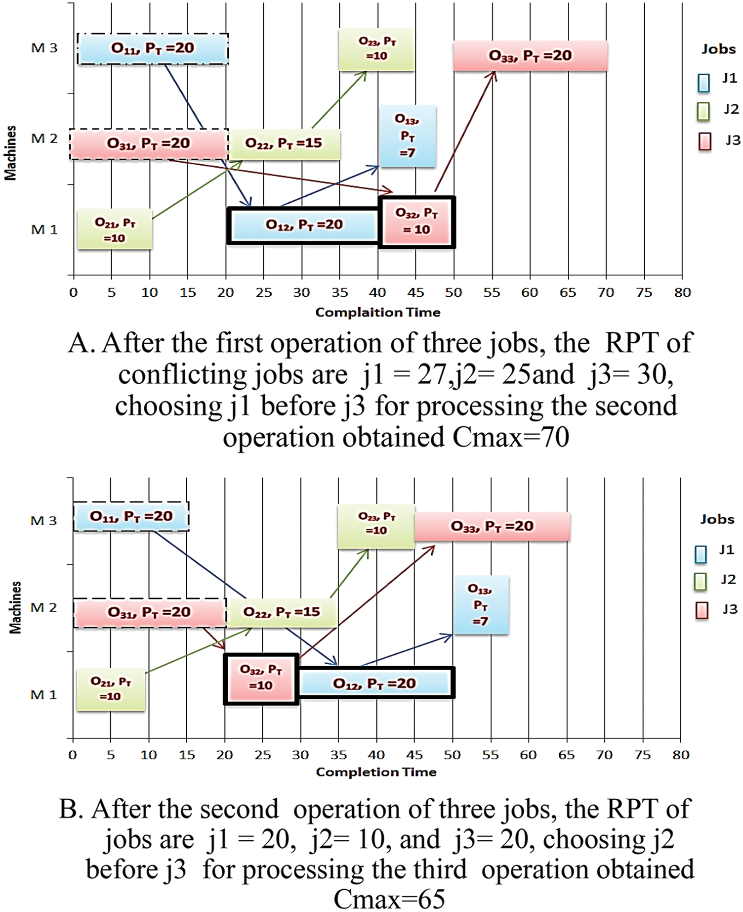
Figure 8: Different completion times obtained by different distributions of job 3

The algorithm proposed can train no of steps to solve the conflicting scheduling based on longest RPT, through 100 episodes number with six steps of problem environment, the model can generate the optimal scheduling and the minimum of maximum completion time can be obtained based on the cumulative rewards generated through training, illustrated in Fig. 9. We noted the stability of the appearance of the reward in the last episode, and it gives near-optimal values of makespan shown in Fig. 10.

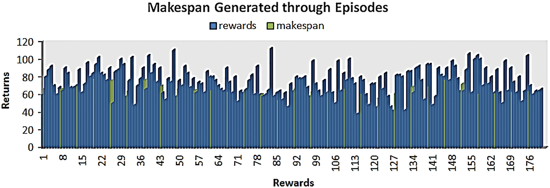
Figure 9: The generated rewards and makespan through training algorithm with no of steps = 6, obtains average Cmax = 65.7 UT

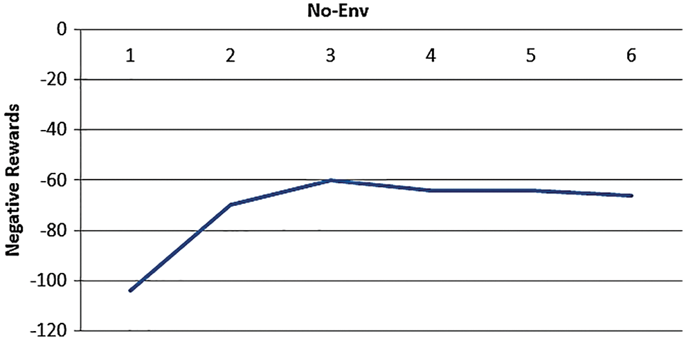
Figure 10: The generated rewards through six environments in the last episode

4.3 Experimentally Using Benchmarks Data Set

4.3.1 Benchmarks Data Set Description

To prove the performance of the proposed algorithm, we evaluate our model on instances of various benchmark dataset sizes benchmarking instances of OR-Library [33], such as 6 × 6, 10 × 10 instances are generated following the well-known Fisher and Thompson (FT) [34], 10 × 5, 15 × 5 and 20 × 5 instances generated also following Lawrence (LA) in Gröflin [35], and Applegate and Cook [36] called ORB instances, they are all size of 10 × 10.

4.3.2 Comparing with Heuristic Rules

Tab. 3 illustrates the comparison between the generalization performance on the makespan of the DRLAC model and other heuristic rules. Shortest Processing Time (SPT), LPT, and FIFO are heuristic rule methods for production sequences; they give an optimal or near-optimal solution for JSP scheduling. We calculate the APD of our techniques from the optimal value of makespan obtained by the Eq. (5):

APDDRLAC=(Cmax−Optimal)/Opimal(5)

The results of makespan in Tab. 3 clear that our DRLAC model in the case of two instances of FT with two different sizes 6 × 6 and 10 × 10 obtains better values than LPT. It obtains good values compared with FIFO and SPT. It is better than SPT, LPT, and FIFO from LA01 to LA04 with size 10 × 5, and from LA11 to LA13 with size 20 × 5. It obtains good values, for instance, LA06 to LA09 with size 15 × 5. By calculating APD for each algorithm shown in Fig. 11, we find that our proposed model performs better than the dispatching rules.

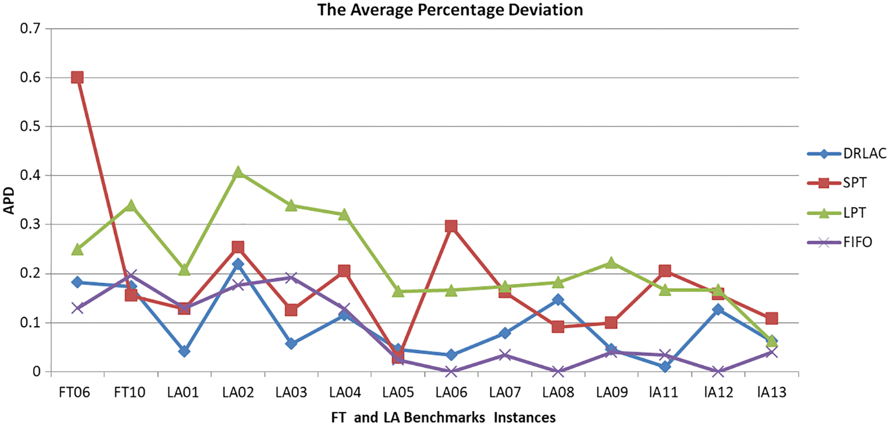
Figure 11: The values of average percentage deviation for DRLAC and dispatching rules

4.3.3 Comparing with Other Trending Approaches

Tab. 4 illustrates the comparison between various approaches such as Genetic algorithm, Deep Reinforcement Learning (DRL) model proposed in [37], A Multi-Agent Reinforcement Learning (MARL) model proposed in [38], and deep deterministic policy gradient (DDPG) proposed in [39], they give an optimal or near-optimal solution of JSP scheduling.

From the results in Tab. 4, for all instances with size 10 × 10, it is clear that our DRLAC model obtains values of makespan better than the Genetic Algorithm (GA).

In addition, DDPG is better than DRL from ORB1 to ORB6 and better than MARL on only four instances of ORB (1, 3, 5, and 7). By calculating the deviation values APD shown in Fig. 12, we find that our proposed model performs well, compared to the different approaches in the types of machine learning. In addition, it performs better than the Meta-heuristic algorithm as GA.

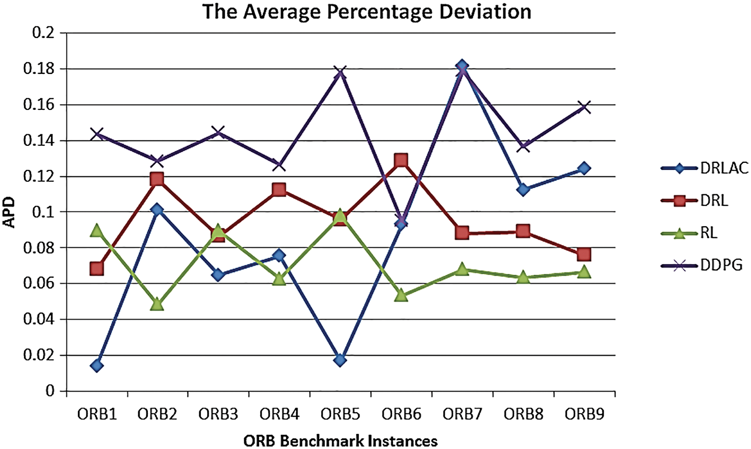
Figure 12: The values of average percentage deviation for DRLAC and various approaches

5  Conclusions and Future Research

The contributions of this paper are summarized as We propose a problem formulation for JSSP as a sequential decision-making problem then, we design the model to represent the scheduling policy based on Graph Isomorphism Network, then we introduced the training algorithm as the actor-critic network algorithm. Our design of a policy network has advantages where first, it can potentially deal with more environments with dynamics and uncertainty systems such as new job arriving and random machine breakdown, by adding or removing certain nodes and/or lines from the disjunctive graphs.

We noted that the GIN representation scheduling for JSSP outperforms practically favored dispatching rules on various benchmark JSSP instances and provides an effective scheduling solution to cope with new job instances. Second, since all nodes shared all parameters in the graph, this property effectively enables generalization to situations of different sizes without training or knowledge transfer.

Finally, through observing the simulation results, we find that if the goal of scheduling is to minimize tardiness or makespan…Etc. Then it may be appropriate to put negative rewards if one or more jobs break their deadlines. For Future work, our model could extend to other shop scheduling problems (e.g., flow-shop). We can introduce another type of graph network as Graph Pointer Networks (GPNs) using reinforcement learning (RL) for tackling the optimization problem.

Funding Statement: The authors received no specific funding for this study.

Conflicts of Interest: The authors declare that they have no conflicts of interest to report regarding the present study.

References

1. Y. Shiue, K. Lee and C. Su, “Real-time scheduling for a smart factory using reinforcement learning approach,” Computers & Industrial Engineering, vol. 125, pp. 604–614, 2018.
2. B. F. Ahmed, M. Saleem, K. Imran, S. Ali, A. Basem et al., “Industry 4.0: Architecture and equipment revolution,” Computers, Materials and Continua, vol. 66, no. 2, pp. 1175–1194, 2021.
3. M. Abdolrazzagh-Nezhad and S. Abdullah, “Job shop scheduling: Classification, constraints and objective functions,” International Journal of Computer and Information Engineering, vol. 11, no. 4, pp. 429–434, 2017.
4. P. Yan, S. Liu, T. Sun and K. Ma, “A dynamic scheduling approach for optimizing the material handling operations in a robotic cell,” Computers & Operations Research, vol. 99, pp. 166–177, 2018.
5. W. Liao and T. Wang, “An optimization approach using in production scheduling with different order.” in Proc. Int. Conf. on Industrial Technology and Management, IEEE, Oxford, United Kingdom, pp. 237–241, 2018.
6. A. Corominas, A. García-Villoria, N. González and R. Pastor, “A multistage graph-based procedure for solving a just-in-time flexible job-shop scheduling problem with machine and time-dependent processing costs,” Journal of the Operational Research Society, vol. 70, no. 4, pp. 620–633, 2019.
7. J. Xu, S. Zhang and Y. Hu, “Research on construction and application for the model of multistage job shop scheduling problem,” Mathematical Problems in Engineering, vol. 2020, pp. 1–20, 2020.
8. C. Wang, Y. Wei, P. So, V. Nguyen and P. Phuc, “Optimization model in manufacturing scheduling for the garment industry,” Computers, Materials & Continua, vol. 71, no. 3, pp. 5875–5889, 2022.
9. S. Yoo and J. Cormac, “Poster: Real-time message scheduling with multiple sinks,” in Proc. Embedded Wireless Systems and Networks, ACM/Junction, United States, pp. 185–186, 2018.
10. P. Manda, A. Hahn, K. Beekman and T. Vision, “Avoiding “conflicts of interest”: A computational approach to scheduling parallel conference tracks and its human evaluation,” PeerJ Computer Science, vol. 5, no. e234, pp. 1–28, 2019.
11. J. Wan, B. Chen, S. Wang, M. Xia, D. Li et al., “Fog computing for energy-aware load balancing and scheduling in smart factory,” IEEE Transactions on Industrial Informatics, vol. 14, no. 10, pp. 4548–4556, 2018.
12. Y. Yang, M. Huang, Z. Yu Wang and Q. Bing Zhu, “Robust scheduling based on extreme learning machine for bi-objective flexible job-shop problems with machine breakdowns,” Expert Systems with Applications, vol. 158, pp. 113545, 2020.
13. A. Kamal, I. Badr and A. Darwish, “Cooperative ant colony algorithm for flexible manufacturing systems,” in SOHOMA, Springer, Cham, pp. 372–383, 2018.
14. M. Romero, A. Fernández, R. García, A. Ponsich and A. Roman, “A heuristic algorithm based on tabu search for the solution of flexible job shop scheduling problems with lot streaming,” in Proc. Genetic and Evolutionary Computation Conf., Kyoto, Japan, pp. 285–292, 2018.
15. I. Hashem, N. Anuar, M. Marjani, E. Ahmed, H. Chiroma et al., “MapReduce scheduling algorithms: A review,” The Journal of Supercomputing, vol. 76, no. 7, pp. 4915–4945, 2020.
16. S. Jha, R. Babiceanu and R. Seker, “Formal modeling of cyber-physical resource scheduling in IIoT cloud environments,” Journal of Intelligent Manufacturing, vol. 31, no. 5, pp. 1149–1164, 2019.
17. Y. Wang, “Adaptive job shop scheduling strategy based on weighted Q-learning algorithm,” Journal of Intelligent Manufacturing, vol. 31, no. 2, pp. 417–432, 2020.
18. Y. Qiu, W. Ji and C. Zhang, “A hybrid machine learning and population knowledge mining method to minimize makespan and total tardiness of multi-variety products,” Applied Sciences, vol. 9, no. 24, pp. 5286, 2019.
19. Y. Li, S. Carabelli, E. Fadda, D. Manerba, R. Tadei et al., “Machine learning and optimization for production rescheduling in industry 4.0,” The International Journal of Advanced Manufacturing Technology, vol. 110, no. 9, pp. 2445–2463, 2020.
20. D. Schlebusch, “Solving the job-shop scheduling problem with reinforcement learning,” 20 [online],Available: http://dx.doi.org/10.26041/fhnw-3437.
21. Z. Zang, W. Wang, Y. Song, L. Lu, W. Li et al., “Hybrid deep neural network scheduler for job-shop problem based on convolution two-dimensional transformation,” Computational Intelligence and Neuroscience, vol. 2019, pp. 1–19, 2019.
22. S. Luo, “Dynamic scheduling for flexible job shop with new job insertions by deep reinforcement learning,” Applied Soft Computing, vol. 91, pp. 106208, 2020.
23. M. Hameed and A. Schwung, “Reinforcement learning on job shop scheduling problems using graph networks,” arXiv preprint, vol. 1, pp. 1–8, 2020.
24. M. Altaf, A. Roshdy and H. AlSagri, “Deep reinforcement learning model for blood bank vehicle routing multi-objective optimization,” Computers, Materials & Continua, vol. 70, no. 2, pp. 3955–3967, 2022.
25. J. Park, J. Chun, S. Kim, Y. Kim and J. Park, “Learning to schedule job-shop problems: Representation and policy learning using graph neural network and reinforcement learning,” International Journal of Production Research, vol. 59, no. 11, pp. 3360–3377, 2021.
26. L. Liu, K. Guo, Z. Gao and J. Li, “Research on the job shop scheduling problem based on digital twin and proximal policy optimization,” Research Square, vol. 9, pp. 1–25, 2022.
27. Z. Dong, T. Ren, J. Weng, F. Qi and X. Wang, “Minimizing the late work of the flow shop scheduling problem with a deep reinforcement learning based approach,” Applied Sciences, vol. 12, no. 5, pp. 2366, 2022.
28. G. Dasoulas, L. Santos, K. Scaman and A. Virmaux, “Coloring graph neural networks for node disambiguation,” arXiv preprint, pp. 2098–2104, 2020.
29. K. Xu, W. Hu, J. Leskovec and S. Jegelka, “How powerful are graph neural networks?,” arXiv preprint arXiv:1810.00826, vol. 3, pp. 1–17, 2019.
30. F. Errica, M. Podda, D. Bacciu and A. Micheli, “A fair comparison of graph neural networks for graph classification,” arXiv preprint arXiv:1912.09893, vol. 3, pp. 1–16, 2022.
31. A. Elsayed, E. Elsayed and K. Eldahshan, “Deep reinforcement learning based actor-critic framework for decision-making actions in production scheduling,” in Proc. Int. Conf. on Intelligent Computing and Information Systems, IEEE, Cairo, Egypt, pp. 32–40, 2021.
32. Github repositories. https://github.com/zcaicaros?tab=repositories.
33. Jobshop Instances. http://jobshop.jjvh.nl/index.php.
34. H. Fisher, “Probabilistic learning combinations of local job-shop scheduling rules,” Industrial Scheduling, pp. 225–251, 1963.
35. H. Gröflin and A. Klinkert, “A new neighborhood and tabu search for the blocking job shop,” Discrete Applied Mathematics, vol. 17, pp. 3643–3655, 2009.
36. D. Applegate and W. Cook, “A computational study of job-shop scheduling,” ORSA Journal of Computing, vol. 3, no. 2, pp. 149–156, 1991.
37. L. Wang, X. Hu, Y. Wang, S. Xu, S. Ma et al., “Dynamic job-shop scheduling in smart manufacturing using deep reinforcement learning,” Computer Networks, vol. 190, pp. 107969, 2021.
38. T. Gabel and M. Riedmiller, “Adaptive reactive job-shop scheduling with reinforcement learning agents,” International Journal of Information Technology and Intelligent Computing, vol. 24, no. 4, pp. 14–18, 2008.
39. C. Liu, C. Chang and C. T. seng, “Actor-critic deep reinforcement learning for solving job shop scheduling problems,” IEEE Access, vol. 8, pp. 71752–71762, 2020.

This work is licensed under a Creative Commons Attribution 4.0 International License, which permits unrestricted use, distribution, and reproduction in any medium, provided the original work is properly cited.