| Computers, Materials & Continua DOI:10.32604/cmc.2022.031027 | |
| Article |
Transfer Learning for Disease Diagnosis from Myocardial Perfusion SPECT Imaging
1Institute of Information Technology, AMST, Hanoi, 11307, Vietnam
2Department of Medical Equipment, 108 Military Central Hospital, Hanoi, 11610, Vietnam
*Corresponding Author: Nguyen Chi Thanh. Email: thanhnc80@gmail.com
Received: 08 April 2022; Accepted: 07 June 2022
Abstract: Coronary artery disease (CAD) is one of the most common pathological conditions and the major global cause of death. Myocardial perfusion imaging (MPI) using single-photon emission computed tomography (SPECT) is a non-invasive method and plays an essential role in diagnosing CAD. However, there is currently a shortage of doctors who can diagnose using SPECT-MPI in developing countries, especially Vietnam. Research on deploying machine learning and deep learning in supporting CAD diagnosis has been noticed for a long time. However, these methods require a large dataset and are therefore time-consuming and labor-intensive. This study aims to develop a cost-effective and high-performance CAD classification model to support doctors in these countries. In this paper, we propose a transfer learning framework for a multi-stage training process with different learning rates. The process consists of two training stages: a warming up stage in which all layers of a pre-trained model (on ImageNet dataset) are frozen; and a fine-tuning stage in which a small amount of the top layers are unfrozen and then retrained with a lower learning rate. The dataset for this study consists of the polar maps from 218 patients. Various popular CNN-based pre-trained models have been investigated, and ResNet152V2-based model has obtained the highest performances with an accuracy of 95.5%, area under the receiver operating characteristic curve (AUC) score 0.932, sensitivity 94.4%, precision 96.4%, and F1-score 95.2%. These performances are competitive or even better than all state-of-the-art approaches in terms of classification accuracy and sensitivity. We also apply the class activation mapping technique to help explain the model’s predictions and increase the model’s reliability, proving capable of assisting the SPECT image readers in the CAD diagnosis.
Keywords: Coronary artery disease; deep learning; transfer learning; SPECT-MPI; polar maps
Coronary artery disease (CAD) is one of the most common pathological conditions and the major global cause of death [1]. According to statistics of the Ministry of Health, in Vietnam, about 200,000 people die from cardiovascular disease each year, accounting for 33% of these deaths. CAD is an atherosclerotic disease usually developed by various causes, including genetic and environmental factors such as unhealthy diet, alcohol use, stress, diabetes, etc. The diagnosis and treatment for CAD require a large proportion of national healthcare budgets, while in low-and middle-income countries, the mortality rate from CAD has increased recently [2]. Thus, cost-effective and accurate diagnosis decisions are crucial for both patients and the socioeconomic status of these countries.
A variety of imaging methods have been used in clinical diagnoses to improve the accuracy, such as single-photon emission computed tomography (SPECT), myocardial perfusion imaging (MPI), positron emission tomography (PET), and cardiovascular computed tomography (CT) [3–8]. According to the European Association of Nuclear Medicine (EANM) [9], SPECT-MPI is a remarkably efficient method regarding CAD diagnosis [3]. This method provides 3D information on the distribution of a radioactive compound within the heart [10], reduces the number of unnecessary angiographies, and enables proper treatment planning [11].
MPI is a non-invasive imaging modality where the uptake of the injected radiopharmaceutical can be measured using SPECT for CAD diagnosis [12]. MPI is a common technique in developed countries because of its outstanding diagnostic quality. However, it is still a complex technique, and the diagnostic results critically depend on the experience and level of expert readers. In developing countries with a large number of patients, such as Vietnam, there is a problem of lacking qualified readers who can make accurate diagnostic decisions using MPI, specifically SPECT-MPI. Machine learning (ML) and deep learning (DL) in medical imaging have become disruptive technologies. We believe that these artificial intelligence (AI) technologies will help improve diagnostic accuracy, reducing healthcare costs and diagnostic time. Moreover, a second reader by AI in CAD diagnosis will be significant for Vietnam cottage hospitals that lack qualified doctors.
Research on deploying ML in supporting CAD diagnosis using SPECT MPI data has been noticed for a decade. From the beginning, the typical ML algorithms such as support vector machine (SVM) [13], artificial neural network (ANN) [14], and ensemble learning [15,16] have been commonly investigated. However, since these ML algorithms require features engineering processes from the raw data (clinical data and SPECT MPI data), ML-based diagnostic models’ performance thoroughly depends on the quality of the features engineering processes. This brings the limitation in improving the diagnostic accuracy. With the ability to automatically extract features from the data, DL tends to be more widely utilized in the context of CAD diagnosis. This trend also comes from the significant improvement in training time and cost for DL in these few years. Thus, several DL-based CAD diagnosis models have been published, and they have improved the diagnostic efficiency quite well. Specifically, in [12], the accuracy of the CAD classification problem reached 0.91 in 2019 from 0.88 in 2013 [13]. However, a DL-based model (and even ML) requires a large dataset to achieve a high accuracy CAD diagnosis. For example, in [13,16–19], the numbers of patients are 957, 1980, 1413, 1638, and 1160, respectively. Furthermore, these such big datasets are not always available. Creating a large enough labeled dataset to deploy an application based on a traditional DL method is time-consuming and labor-intensive [20]. Meanwhile, all data sets used in related studies are not published. Therefore, it is significantly challenging for Vietnamese researchers to have a large enough data set to use the above methods to build a diagnostic model for Vietnamese people. Fortunately, Transfer Learning, a DL technique, can help address this limitation.
Instead of building a new convolutional neural network (CNN) architecture from scratch, which is the traditional strategy in DL, an alternative technique called Transfer Learning (TL) [21] has recently become more popular. TL will offer many benefits: a higher starting accuracy, faster convergence, and higher asymptotic accuracy with a small dataset. By TL, we can transfer knowledge of a well-trained CNN model on a large dataset (e.g., ImageNet [22]) to solve classification problems in medical image analysis, particularly in CAD diagnosis.
In medical image analysis, TL has shown its effectiveness for almost all anatomical sites and image types, such as X-Ray (X-radiation) images of the skeletal system [23, 24], breast X-Ray [25,26], lung X-ray [4,27], breast MRI (Magnetic Resonance Imaging) [28,29], brain MRI images [30,31], CT (Computed tomography) scan images [32], OCT (Optical Coherence Tomography) images [33], and skin lesion images [34].
In the context of SPECT MPI images, TL is considered a method for CAD prediction in [3,10,35]. However, the limitation of these previous studies is adopting a simple FT strategy that unfreezes some specific layers before retraining the pre-trained CNN model [3]. They did not consider the differences in the domain between SPECT MPI dataset and the ImageNet dataset, so the achieved models did not have full the benefits of TL.
Moreover, the dataset used in the related works can be organized into two categories: sliced images and polar maps. The sliced images contain various helpful information for the CAD diagnosis, but using the sliced images to diagnose is very complicated and requires a highly experienced and expert reader to make an accurate prediction. In contrast, polar images, synthesized from sliced images, provide a better overview of the heart and are easier to read and diagnose than sliced images. A CAD diagnosis using polar images is more explainable than using sliced images because of the ability to integrate visualization techniques such as Class activation mapping (CAM) [36]. The visualization techniques will significantly assist the doctors, especially in cottage hospitals in Vietnam, in diagnosing and explaining the model’s prediction to patients. However, while the existing methods for sliced images bring a high performance (accuracy of 93.4% in [3] and accuracy of 94% in [10]), the method for polar images is not much effective (accuracy of 75% in [35]).
In this paper, we propose a transfer learning framework focusing on an accurate CAD diagnosis from polar images. The main contributions of this paper are as follows:
i) We propose a multi-stage transfer learning framework with an original learning rate scheduler from SPECT MPI polar maps.
ii) We compare our method with different 05 strategies to evaluate the effectiveness of the proposed transfer learning framework. Moreover, we adopt CAM to visualize the prediction of the model as a way to evaluate the performance.
iii) We evaluate the proposed method using 15 pre-trained models, and all of them show high performances with accuracy > 86.4%
iv) The proposed method provides state-of-the-art accuracy and sensitivity compared to related works.
The organization of this paper is structured as follows. Section 2 reviews related works on CAD classification using. Section 3 describes the methodology and materials. Section 4 presents the experimental results. In Section 5, the proposed method results are discussed and compared to the related works. Finally, the conclusions of this paper are presented in Section 5.
Recent years, some transfer learning methods have been proposed for supporting CAD diagnosis. As mentioned early, based on the data, the existing related works can be organized into two categories: sliced images and polar maps.
For sliced images, Berkaya et al. proposed two different TL-based models [10]. The first one uses pre-trained deep CNNs as feature extractors and SVM as a classifier, called Feature Extractor (FE). The second one uses a simple Fine-tuning (FT) strategy to retrain deep CNNs with a new fully-connected layer as the classifiers. The results on SPECT dataset, including the summed stress and rest slice images of 192 patients, show that VGG16 pre-trained network with the SVM deep feature shallow performed the best classification accuracy up to 0.94. On the contrary, the accuracy of the second model using FT was not very high, only 0.86.
Papandrianos et al. introduced an approach of TL for CAD diagnosis [3]. Instead of using popular pre-trained deep CNNs (VGG16, ResNet, GoogLeNet,…), they applied the RGB-CNN model, which they proposed in the domain of bone scintigraphy, to classify CAD or not by using SPECT sliced images from 224 patients. The accuracy 93.4 ± 2.81%, AUC (area under the receiver operating characteristic (ROC) curve) score = 0.936 were achieved. The results show that implementing a deep learning classification model utilizing TL can help to improve the CAD diagnosis significantly.
Instead of sliced images, Apostolopoulos et al. used polar maps from 216 patients to predict CAD [35]. They adopted data augmentation to expand the training data, including two attenuation correction images, two non-attenuation corrections images (stress and rest condition), and concatenated them to create a dataset as the input of VGG16 based classification model. As a result, the model achieved an accuracy of 75%, a sensitivity of 0.75, and a specificity of 0.73.
From the related works above, compared with ML and DL methods, TL does not require a large dataset. However, while the existing methods for sliced images bring very high performance, the method for polar images is not much effective. To address this problem, we focus on developing a TL framework that could achieve high performance on a small dataset.
3.1 Overview of the Proposed Method
This subsection introduces the overview of the proposed framework for CAD diagnosis from SPECT MPI polar maps. Firstly, the polar images will be preprocessed in the data preparation step. Then, we create a classification model using a pre-trained model and train the model in two stages: Warming up stage and Fine-tuning stage with differential learning rates. The difference between the proposed method and the related works [3,10,22] is using two training and testing times. In addition, to optimize the advantages of TL, we proposed an original learning rate scheduler (this will be described below). Furthermore, we adopt a greedy algorithm to determine the best model at each stage: selecting the best model which showed the highest accuracy at every stage. The flow diagram is described in Fig. 1, and the details are explained in the following subsections.
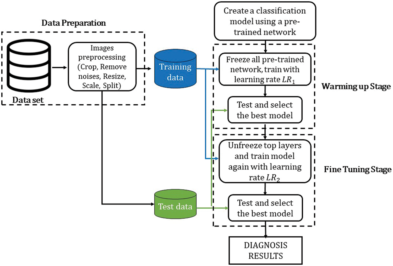
Figure 1: The flow diagram of the proposed method
3.2 Dataset and Data Preparation
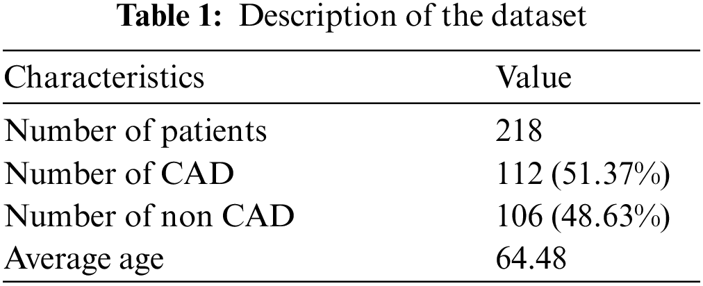
The dataset used in this paper corresponds to a retrospective review that includes SPECT MPI polar maps from 218 patients collected in the Department of Nuclear Medicine of 108 Hospital, Hanoi, Vietnam. This dataset was obtained after a processing procedure and consultation with many technicians and doctors. The dataset consists of AC (attenuation correction) images and NAC (non-attenuation correction) images in both stress and rest conditions. This study only used the stress AC images. The description of the dataset is summarized in Tab. 1.
In the data preparation phase, a raw polar map image is processed as follows:
i) Crop image: The polar images in the dataset were reconstructed from SPECT MPI sliced images by specialized software. The reconstructed polar map image is a high-resolution jpeg image (1640 × 1068), so it is required to crop to pick up the essential area and reduce noises as much as possible.
ii) Remove noises: As shown in Fig. 2a, the reconstructed polar map image has a white text line showing the information, including image type, scanning time, or machine name. These noises may affect the model’s performance. After cropping and removing noises, a clean image containing only a polar map is obtained. A sample of this image is shown in Fig. 2b.
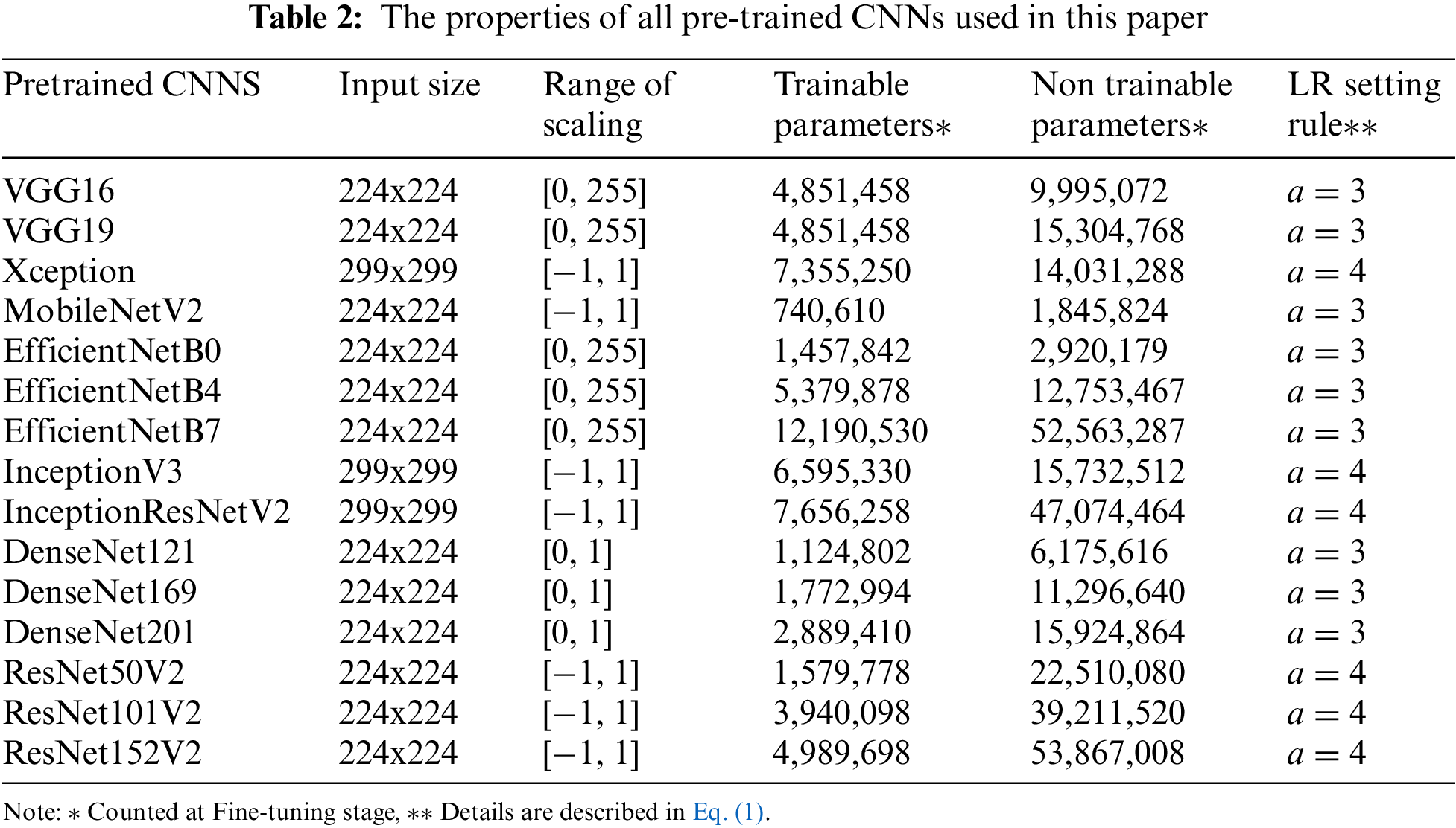
iii) Resize and Scale: Images are resized and scaled (if need be) to fit each pre-trained CNNs. For example, for ResNetV2, the input size has to be 224x224, and the value in each pixel has to be scaled between [−1, 1] [37]. Tab. 2 shows the properties of all pre-trained CNNs used in this paper.
iv) Split: Split the dataset into training data (80%) and test data (20%) for each class.
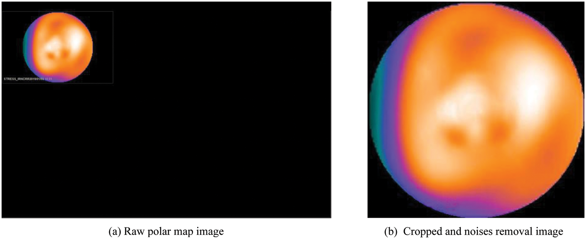
Figure 2: An example of a polar map image before and after processing
3.3 Pre-trained Deep CNN Models
Instead of developing a deep CNN from scratch, we used 15 pre-trained deep CNNs, which are well-trained on ImageNet [22] (more than 1 million images for 1000 classes). The properties of the pre-trained deep CNNs are described in Tab. 2. As shown in Fig. 3, the architecture of the proposed model consists of CNN-based layers for features extraction and fully connected (FC) layers, which are reconstructed for the CAD classification. In particular, we replaced the original FC layers (for ImageNet with 1000 classes) with new FC layers to classify CAD or non CAD (binary class). Hyper-parameters (number units per layer, dropout rate) of these new FC layers are optimized by the Hyperband algorithm [38].
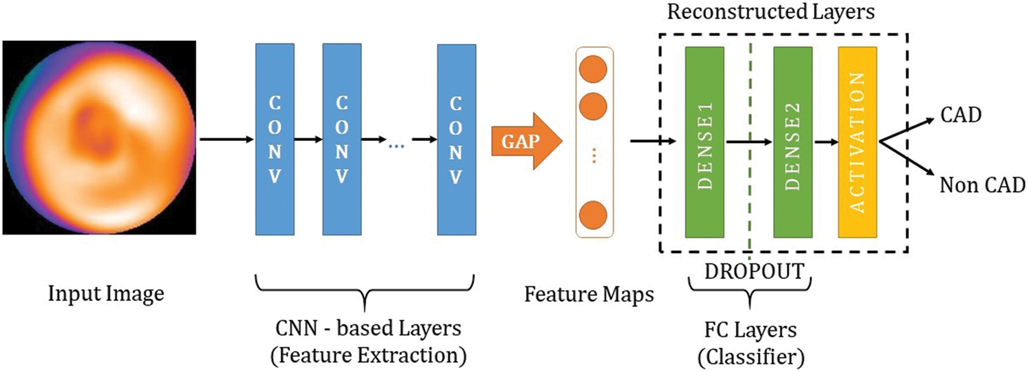
Figure 3: The overall architecture of the proposed models
Since the dataset is small, we use Global Average Pooling (GAP) instead of Flatten function at the end of the feature extraction to prevent overfitting [39]. Furthermore, the GAP is more native to the convolution structure by enforcing correspondences between feature maps and categories so the feature maps can be easily interpreted as category confidence maps [40].
3.4 Proposed Transfer Learning Process
As mentioned in Section 2.1, the model in our framework was trained and tested on a 2-stage process as follows:
i) Warming up stage: By using the well-trained models on the ImageNet dataset, they are expected to extract the critical features of the polar maps. Hence, the reconstructed layers (classifier) need to be trained at first to determine how well the CNN-based layers can extract the critical features. Thus, we froze all the CNN-based layers, left only the FC layers trainable, then trained the model for 100 epochs. The training data was fed by batch. While all of the batches were fed and a training epoch was complete, the weights were saved. Here, we use the following greedy algorithm to determine the best model: after all training epochs were completed, the trained model was used to determine the best model that showed the highest accuracy among all saved weights. The best model was selected for the next stage.
ii) Fine-tuning stage: Since there are differences between SPECT MPI dataset and ImageNet, some top layers of the model must be retrained to fit the weights to our dataset. Hence, we unfroze some top layers of the best model that was selected at Warming up stage, then retrained the model with a smaller learning rate (LR) for 30 epochs. The number of the trainable top layers is set to be proportional to the depth of the pre-trained CNN and inversely proportional to the number of trainable parameters. In particular, this value was set to a small value so that smaller than 1/3 of the total layers and the number of the trainable parameters was also smaller than 1/3 of the total parameters. The model testing and selection were executed in the same way as in Warming up stage.
Additionally, we adopted a differential LR approach in the training process, where the LR is determined on a per-layer basis. The bottom layers will then have a very small LR or be set as non-trainable layers. These generalize quite well, responding principally to edges, blobs, and other low-level features, whereas the top layers respond to high-level features a higher learning rate [41]. In this paper, we use the following LR setting rule:
where
3.5 Class Activation Mapping for Visualization
It is challenging to explain CNN black-box models and understand their predictions. It is beneficial to ensure that the neural network concentrates on appropriate parts of the image. Visualization of the feature maps is one of the most common practices to understand and trust the decision-making of the CNNs based models. In this paper, we used Class Activation Mapping (CAM) [36], also known as a heatmap, to determine the discriminative image regions by taking the values from the gradients in the model’s final feature layer.
This paper focuses on the image classification problem considering the classification of SPECT MPI polar maps into two classes: CAD and non CAD. The performances were evaluated by accuracy (Acc), sensitivity (Sen), specificity (Spe), precision (Pre), F1-score, and area under the ROC curve (AUC).
The experimental simulations were implemented using Keras and TensorFlow frameworks on a computer with 16 Intel Xeon CPUs running at 3.40 GHz and an NVIDIA Quadro RTX 4000 GPU. The experimental settings of pre-trained CNNs used in this paper are shown in Tab. 2.
4.1 Comparison of Different Pre-Trained CNNs
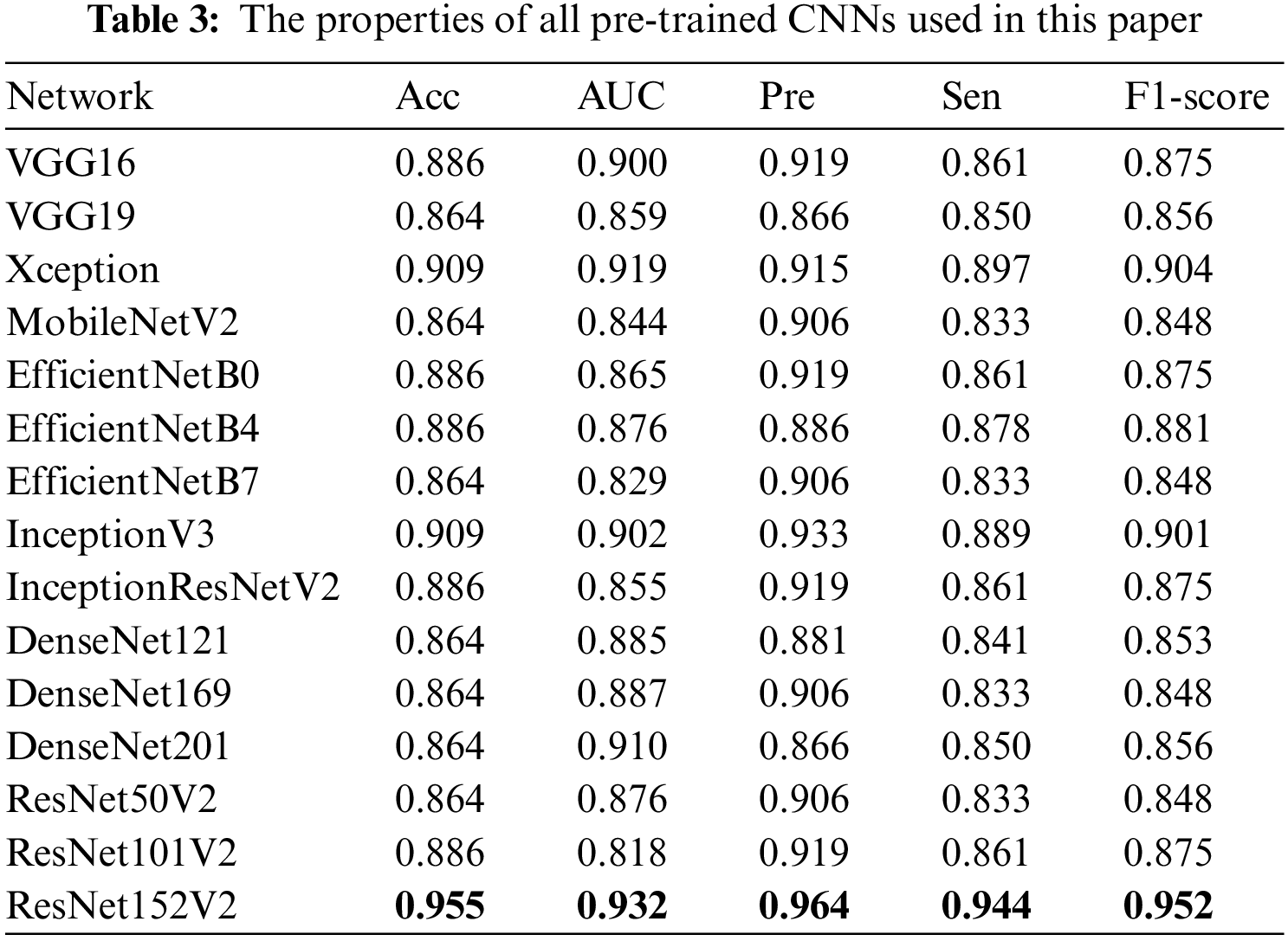
Tab. 3 presents the performances for each of the 15 models. We used all the most popular pre-trained CNNs such as VGG, Xception, EfficientNet, Inception, DenseNet, ResNet, and the deeper version (VGG19, ResNet152V2, etc). The results demonstrated that all the pre-trained CNNs models showed very high performances with Acc > 86.4%. Moreover, we found that ResNet152V2-based model showed the best performances for all metrics: Acc 95.5%, AUC 0.932, Sen 94.4%, Pre 96.4%, and F1-score 95.2%.
4.2 Comparison of Different Transfer Learning Strategies
Firstly, to evaluate the effectiveness of the proposed TL framework, we conducted experiments in the following six TL strategies with the ResNet152V2 model:
• Strategy 1: Training the model from scratch (not using pre-trained weights on ImageNet) for 100 epochs.
• Strategy 2: Using pre-trained weights, setting all layers trainable, then training the model for 100 epochs.
• Strategy 3: Using pre-trained weights, freeze the bottom layers (first 200 layers), leaving the top layers and the reconstructed layers trainable, then train the model for 100 epochs.
• Strategy 4: Warming up stage only.
• Strategy 5: Fine-tuning stage only.
• Strategy 6: The proposed method: Warming up stage + Fine-tuning stage with a differential LR approach.
Fig. 4 shows the evolution of accuracy and loss plots at each strategy in the case of ResNet152V2-based model. As shown in Figs. 4a, 4b, and 4c, overfitting occurred after a few epochs. The reason is that a deeper model and more trainable layers would make the model prone to overfitting. On the contrary, by freezing all CNN-based layers, only the reconstructed layers (a single layer and an output layer) were trainable, and the model avoided overfitting (Fig. 4d). In strategy 4, the best model that showed the highest accuracy with as small as possible overfitting was retrained in the Fine-tuning stage (strategy 6). Fig. 4f showed that both training and testing Acc were improved. The overfitting also did not appear in strategy 5 when only the first few top layers were trained. However, as shown in Tab. 4, Strategy 5 provided better performances than Strategy 3 did but worse than Strategy 4 did. A small LR causes the classifier layers not to update the appropriate weights, while a large LR causes the well-trained weights of the top layers to be changed a lot. This problem was solved by Strategy 6. Fig. 4f showed that fine-tuning some top layers improved both training and testing Acc with a small LR.
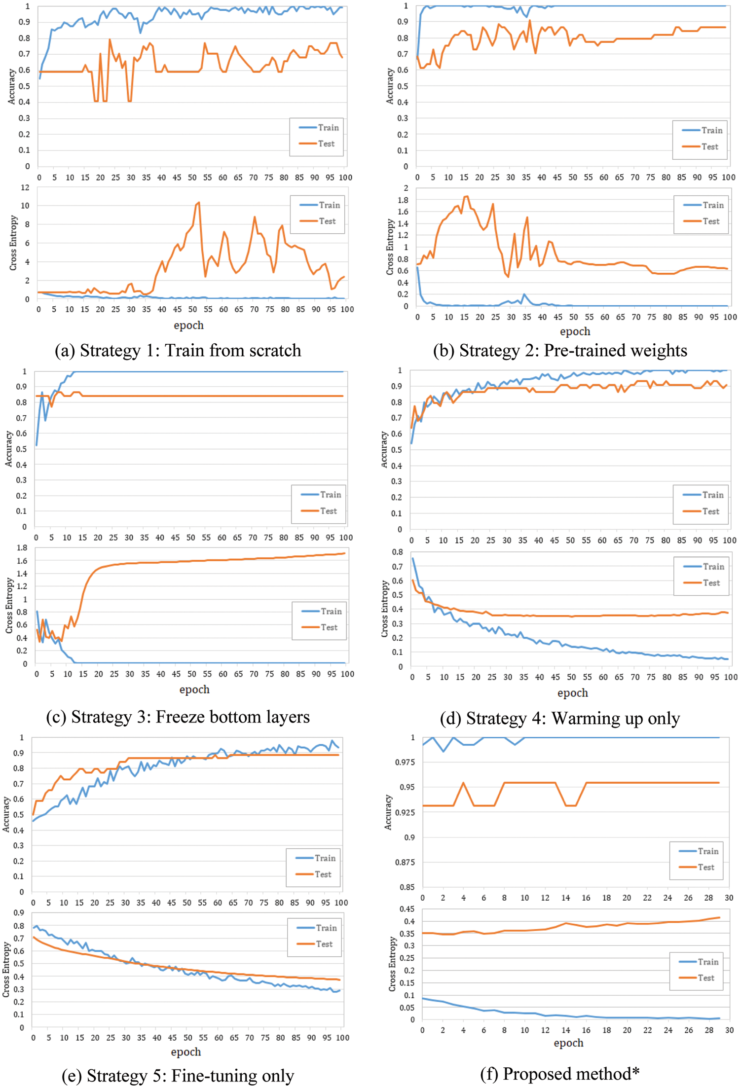
Figure 4: Accuracy and loss plots at each strategy in the case of the ResNet152V2-based model. LR rule: a = 4. *The best model achieved at strategy 4 was then fined tuning
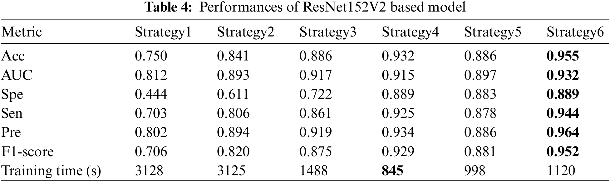
As shown in Tab. 4, the TL strategy in which the bottom layers were frozen during training (strategy 3, 4, 5, and 6) showed higher Acc and better training time. Furthermore, unfreezing some top layers and retraining the model one more stage with a small LR (Fine-tuning stage) could make the model adapt better to the polar maps dataset. The proposed method with ResNet151V2 improved the performances significantly in all metrics: Acc up to 0.955 from 0.75 while training from scratch and 0.932 while training in only warming up stage; AUC up to 0.932, Sen up to 0.944, Spe up to 0.889, Pre up to 0.964, and F1-score up to 0.952.
Fig. 5 presents a comparison of the diagnosis results using the CAM technique. The left images are original images in which the upper is non CAD, and the lower is CAD. The center one is the heatmap created by CAM with the prediction results: CAD (label 0) or non CAD (label 1) with a probability score. The right one represents the activation regions. The areas with higher intensity in these two images are the heatmap with the highest activation response from the last convolutional layer. As can be seen, while at other strategies, the model seemed to make a wrong decision by looking at the black area (strategy 1 and 5) or scattering the whole image (strategy 2, 3, and 4), the proposed method (strategy 6) enables the model to focus on lower radiotracer activity area (purple area) in the 4th quadrant for the CAD classification. These results seem to be close to the diagnosis of the experts. In addition, with the softmax activation function, the model shows a prediction with its probability (below the center heatmap). The probability of the prediction and the heatmaps will support the readers make faster and more accurate decisions.
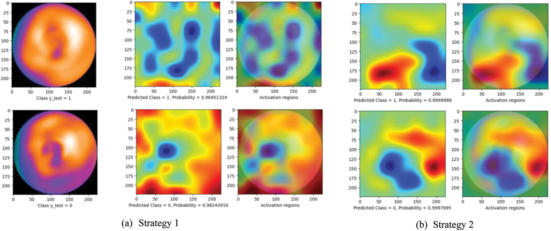
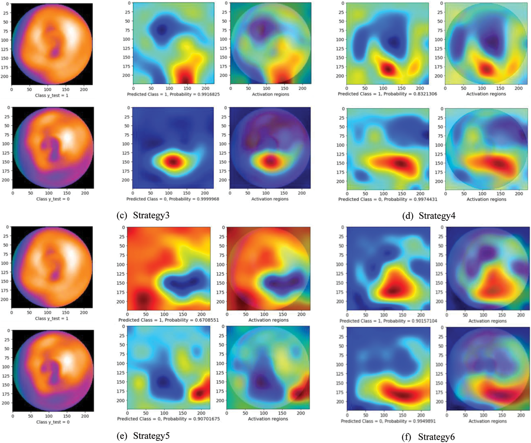
Figure 5: Diagnosis results using CAM technique. The left images are original images in which the upper is non CAD, and the lower is CAD. The center one is the heatmap created by CAM with the prediction results: CAD (label 0) or non CAD (label 1) with a probability score. The right one represents the activation regions
A comparison to the related works in CAD classification using Machine Learning (ML) and Deep Learning (DL) methods is presented in Tab. 5.
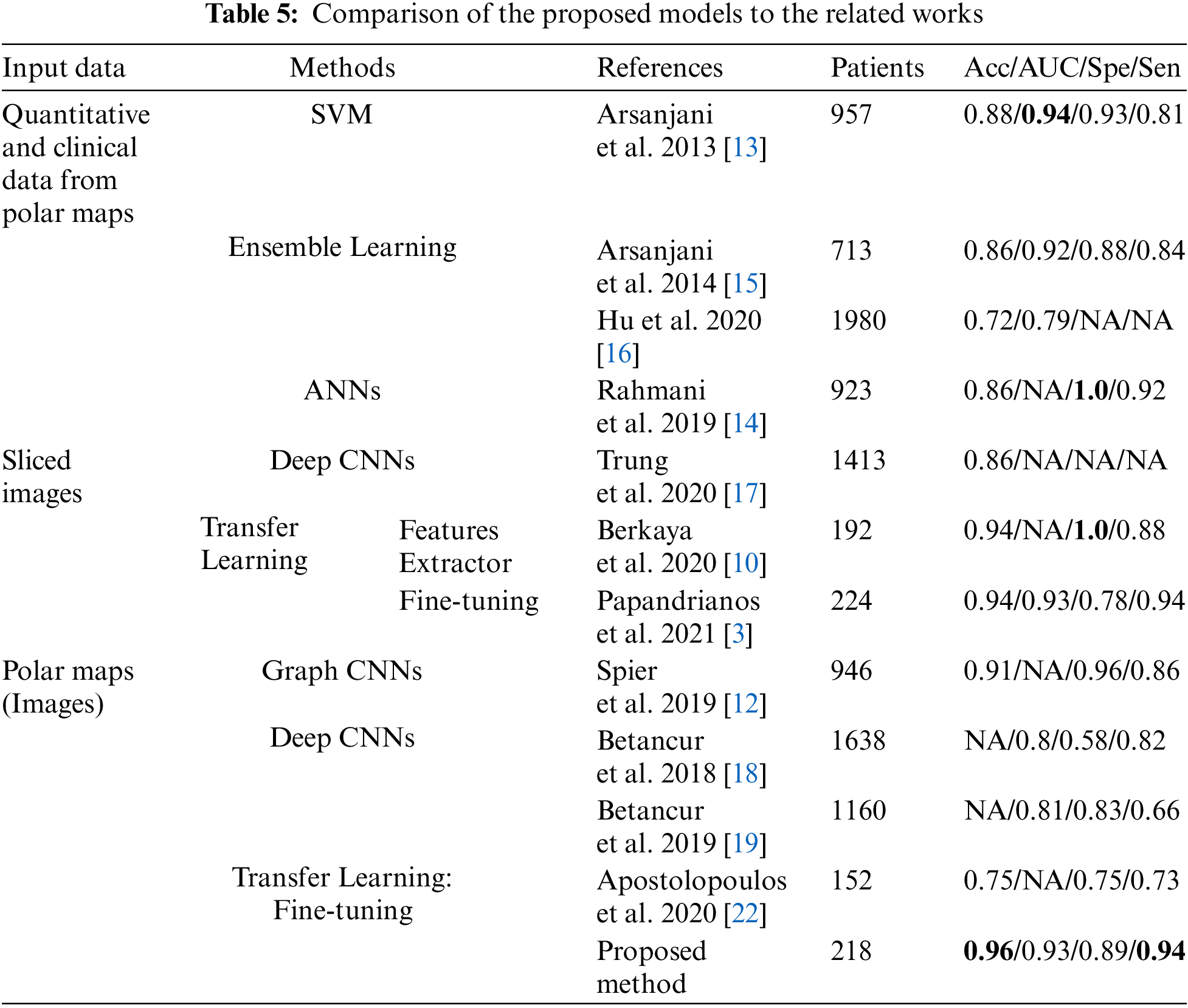
As mentioned early, in the related works using ML, the models’ performance thoroughly depends on the quality of the features extraction process. Some of the related works focused on improving the quality of this process to archive high performances, especially the AUC up to 0.94 [13] and Spe up to 1.0 [14]. Nevertheless, the lack of an automatic features extraction (FE) process is a significant drawback that made these methods less popular in recent years. On the contrary, as there is no need for a feature extraction process, DL has become more prevalent in recent years. Among many research on DL for CAD classification, the highlight is the study on the deployment of graph convolutional neural networks (Graph CNNs) by Spier et al. [12]. This study improved the performances significantly: Acc up to 91% and Spe up to 96%, which was state-of-the-art at that time.
Compared with the DL methods, TL method requires fewer data and still gives high performance. The reason is to use the well-trained models on ImageNet, which has more than 1 million images for 1000 classes. Thus, TL is considered an effective method to solve the problem of data shortage in medical imaging.
In related works, while the TL methods for slided images have been archived with very high performance (Acc 94% in [3,10]), TL method for polar maps proposed by Apostolopoulos et al. [35] has not yielded high efficiency. Focusing on this problem, we proposed a multi-stage transfer learning framework to optimize the advantages of TL concept. Compared with the research of Apostolopoulos et al., the proposed method outperformed [35] in every metric: Acc 95.5% and 75%, Spe 0.89 and 0.75, Sen 0.94 and 0.73.
Moreover, compared with the other related works in CAD classification, the proposed method obtained the highest classification accuracy of 95.5% and highest sensitivity of 94.4%. In particular, among the related works using polar maps, our model showed the highest performances in almost metrics, even compared to the study of Spier et al. [12].
However, this work has some limitations that need to be considered in future works. Firstly, the proposed method has been evaluated on only one dataset due to the lack of available datasets. Secondly, we have disregarded clinical data (such as chest pain and shortness of breath) and demographic data (such as age and sex), which might improve the CAD diagnosis.
This study proposed a multi-stage transfer learning framework for coronary artery disease diagnosis by polar maps. In the training process, we use different learning rates for each stage. We fine-tune a small amount of the top layers selectively to optimize the valuable benefits of the transfer learning technique. We also investigated our framework on various popular CNN-based pre-trained models, and ResNet152V2-based model obtained the highest performances with the accuracy of 95.5%, AUC 0.932, sensitivity 94.4%, precision 96.4%, and F1-score 95.2%. To the best of our knowledge, the results are competitive or even better performances than all state-of-the-art approaches regarding classification accuracy and sensitivity. Consequently, the proposed method can be used to assist SPECT polar maps readers in coronary artery disease diagnosis.
In future works, we intend to improve the performances of the proposed model by using ensemble learning in which the outcomes of multiple pre-trained models can be strategically combined. We also plan to consider combining clinical data, demographic data, and polar maps to deploy a deep diagnostic model comparable to clinicians and SPECT image expert readers.
Funding Statement: This research is funded by AMST under grant number ĐTVCN.01.21/CNTT.
Conflicts of Interest: The authors declare that they have no conflicts of interest to report regarding the present study.
References
1. A. Cassar, D. Holme, C. S. Rihal and B. J. Gersh, “Chronic coronary artery disease: Diagnosis and management,” in Mayo Clinic Proceedings, vol. 84, no. 12, pp. 1130–1146, 2009. [Google Scholar]
2. who. int. Cardiovascular diseases [Online]. Available: https://www.who.int/health-topics/cardiovascular-diseases. Accessed on Dec. 15, 2021. [Google Scholar]
3. N. Papandrianos and E. Papageorgiou, “Automatic diagnosis of coronary artery disease in SPECT myocardial perfusion imaging employing deep learning,” Applied Sciences, vol. 11, no. 14, pp. 6362, 2021. [Google Scholar]
4. W. Wang, H. Liu, J. Li, H. Nie and X. Wang, “Using CFW-net deep learning models for X-ray images to detect COVID-19 patients,” International Journal of Computational Intelligence Systems, vol. 14, no. 1, pp. 199–207, 2021. [Google Scholar]
5. J. N. Talbot, F. Paycha and S. Balogova, “Diagnosis of bone metastasis: Recent comparative studies of imaging modalities,” Quarterly Journal of Nuclear Medicine and Molecular Imaging, vol. 55, no. 4, pp. 374–410, 2011. [Google Scholar]
6. K. Doi, “Computer-aided diagnosis in medical imaging: Historical review, current status and future potential,” Computerized Medical Imaging and Graphics, vol. 31, no. 4–5, pp. 198–211, 2007. [Google Scholar]
7. G. J. O’Sullivan, F. L. Carty and C. G. Cronin, “Imaging of bone metastasis: An update,” World Journal of Radiology, vol. 7, no. 8, pp. 202–211, 2015. [Google Scholar]
8. C. Y. Chang, C. M. Gill, F. J. Simeone, A. K. Taneja, A. J. Huang et al., “Comparison of the diagnostic accuracy of 99 m-tc-MDP bone scintigraphy and 18 F-FDG PET/CT for the detection of skeletal metastases,” Acta Radiologica, vol. 57, no. 1, pp. 58–65, 2016. [Google Scholar]
9. T. V. D. Wyngaert, K. Strobel, W. U. Kampen, T. Kuwert, W. V. D. Bruggen et al., “The EANM practice guidelines for bone scintigraphy,” European Journal of Nuclear Medicine and Molecular Imaging, vol. 43, no. 9, pp. 1723–1738, 2016. [Google Scholar]
10. S. K. Berkaya, I. A. Sivrikoz and S. Gunal, “Classification models for SPECT myocardial perfusion imaging,” Computers in Biology and Medicine, vol. 123, no. 103893, 2020. [Google Scholar]
11. E. B. N. Alexanderson, S. E. Bouyoucef, M. Dondi, S. Dorbala, A. J. Einstein et al., “Nuclear cardiology: Guidance on the implementation of SPECT myocardial perfusion imaging,” IAEA Human Health Series, vol. 23, (Rev.1pp. 19–39, 2016. [Google Scholar]
12. N. Spier, S. Nekolla, C. Rupprecht, M. Mustafa, N. Navab et al., “Classification of polar maps from cardiac perfusion imaging with graph-convolutional neural networks,” Scientific Reports, vol. 9, no. 7569, pp. 1–8, 2019. [Google Scholar]
13. R. Arsanjani, Y. Xu, D. Dey, M. Fish, S. Dorbala et al., “Improved accuracy of myocardial perfusion SPECT for the detection of coronary artery disease using a support vector machine algorithm,” Journal of Nuclear Medicine, vol. 54, no. 4, pp. 549–555, 2013. [Google Scholar]
14. R. Rahmani, P. Niazi, M. Naseri, M. Neishabouri, S. Farzanefar et al., “Improved diagnostic accuracy for myocardial perfusion imaging using artificial neural networks on different input variables including clinical and quantification data,” Spanish Journal of Nuclear Medicine and Molecular Imaging, vol. 38, no. 5, pp. 275–279, 2019. [Google Scholar]
15. R. Arsanjani, D. Dey, T. Khachatryan, A. Shalev, S. W. Hayes et al., “Prediction of revascularization after myocardial perfusion SPECT by machine learning in a large population,” Journal of Nuclear Cardiology, vol. 22, no. 5, pp. 877–884, 2014. [Google Scholar]
16. L. H. Hu, J. Betancur, T. Sharir, A. J. Einstein, S. Bokhari et al., “Machine learning predicts per-vessel early coronary revascularization after fast myocardial perfusion SPECT: Results from multicentre REFINE SPECT registry,” European Heart Journal-Cardiovascular Imaging, vol. 21, no. 5, pp. 549–559, 2020. [Google Scholar]
17. N. T. Trung, N. T. Ha, N. T. Thuan and D. H. Minh, “A deep learning method for diagnosing coronary artery disease using SPECT images of heart,” Journal of Science and Technology, vol. 144, pp. 22–27, 2020. [Google Scholar]
18. J. Betancur, F. Commandeur, M. Motlagh, T. Sharir, A. J. Einstein et al., “Deep learning for prediction of obstructive disease from fast myocardial perfusion SPECT,” JACC: Cardiovasc. Imaging, vol. 11, no. 11, pp. 1654–1663, 2018. [Google Scholar]
19. J. Betancur, L. H. Hu, F. Commandeur, T. Sharir, A. J. Einstein et al., “Deep learning analysis of upright-supine high-efficiency SPECT myocardial perfusion imaging for prediction of obstructive coronary artery disease: A multicenter study,” Journal of Nuclear Medicine, vol. 60, no. 5, pp. 664–670, 2018. [Google Scholar]
20. A. Borjali, A. F. Chen, O. K. Muratoglu, M. A. Morid and K. M. Varadarajan, “Detecting total hip replacement prosthesis design on plain radiographs using deep convolutional neural network,” Journal of Orthopaedic Research, vol. 38, no. 7, pp. 1465–1471, 2020. [Google Scholar]
21. S. J. Pan and Q. Yang, “A survey on transfer learning,” IEEE Transactions on Knowledge and Data Engineering, vol. 22, no. 10, pp. 1345–1359, 2010. [Google Scholar]
22. J. Deng, W. Dong, R. Socher, L. J. Li, K. Li et al., “ImageNet: A large-scale hierarchical image database,” in Proc. of IEEE Computer Vision and Pattern Recognition, United States of America, pp. 248–255, 2009. [Google Scholar]
23. A. Z. Abidin, B. Deng, A. M. DSouza, M. B. Nagarajan, P. Coan et al., “Deep transfer learning for characterizing chondrocyte patterns in phase contrast X-ray computed tomography images of the human patellar cartilage,” Computers in Biology and Medicine, vol. 95, pp. 24–33, 2018. [Google Scholar]
24. J. S. Yu, S. M. Yu, B. S. Erdal, M. Demirer, V. Gupta et al., “Detection and localisation of hip fractures on anteroposterior radiographs with artificial intelligence: Proof of concept,” Clinical Radiology, vol. 75, no. 3, pp. 237.e1–237.e9, 2020. [Google Scholar]
25. X. Zhang, Y. Zhang, E. Y. Han, N. Jacobs, Q. Han et al., “Classification of whole mammogram and tomosynthesis images using deep convolutional neural networks,” IEEE Trans Nanobioscience, vol. 17, no. 3, pp. 237–242, 2018. [Google Scholar]
26. H. Li, M. L. Giger, B. Q. Huynh and N. O. Antropova, “Deep learning in breast cancer risk assessment: Evaluation of convolutional neural networks on a clinical dataset of full-field digital mammograms,” Journal of Medical Imaging (Bellingham), vol. 4, no. 4, pp. 0413041–0413046, 2017. [Google Scholar]
27. Q. H. Nguyen, B. P. Nguyen, S. D. Dao, B. Unnikrishnan, R. Dhingra et al., “Deep learning models for tuberculosis detection from chest X-ray images,” in Proc. of 26th Int. Conf. on Telecommunications, Vietnam, pp. 381–385, 2019. [Google Scholar]
28. Z. Zhu, E. Albadawy, A. Saha, J. Zhang, M. R. Harowicz et al., “Deep learning for identifying radiogenomic associations in breast cancer,” Computers in Biology and Medicine, vol. 109, pp. 85–90, 2019. [Google Scholar]
29. Z. Zhu, M. Harowicz, J. Zhang, A. Saha, L. J. Grimm et al., “Deep learning analysis of breast MRIs for prediction of occult invasive disease in ductal carcinoma in situ,” Computers in Biology and Medicine, vol. 115, no. 103498, 2019. [Google Scholar]
30. C. Zhang, K. Qiao, L. Wang, L. Tong, G. Hu et al., “A visual encoding model based on deep neural networks and transfer learning for brain activity measured by functional magnetic resonance imaging,” Journal of Neuroscience Methods, vol. 325, no. 108318, 2019. [Google Scholar]
31. M. Maqsood, F. Nazir, U. Khan, F. Aadil, H. Jamal et al., “Transfer learning assisted classification and detection of Alzheimer’s diseases stages using 3D MRI scans,” Sensors (Basel), vol. 19, no. 11, 2019. [Google Scholar]
32. J. H. Lee, E. J. Ha and J. H. Kim, “Application of deep learning to the diagnosis of cervical lymph node metastasis from thyroid cancer with CT,” European Radiology, vol. 29, no. 10, pp. 5452–5457, 2019. [Google Scholar]
33. K. T. Islam, S. Wijewickrema and S. O’Leary, “Identifying diabetic retinopathy from OCT images using deep transfer learning with artificial neural networks,” in Proc. of IEEE 32nd Int. Symp. on Computer-Based Medical Systems, Spain, pp. 281–286, 2019. [Google Scholar]
34. A. R. Lopez, X. Giro-I-Nieto, J. Burdick and O. Marques, “Skin lesion classification from dermoscopic images using deep learning techniques,” in Proc. of 13th IASTED Int. Conf. on Biomedical Engineering; Institute of Electrical and Electronics Engineers Inc., Austria, pp. 49–54, 2017. [Google Scholar]
35. I. D. Apostolopoulos, N. D. Papathanasiou, T. Spyridonidis and D. J. Apostolopoulos, “Automatic characterization of myocardial perfusion imaging polar maps employing deep learning and data augmentation,” Hellenic Journal of Nuclear Medicine, vol. 23, no. 2, pp. 125–132, 2020. [Google Scholar]
36. B. Zhou, A. Khosla, A. Lapedriza, A. Oliva and A. Torralba, “Learning deep features for discriminative localization,” in Proc. of IEEE Conf. on Computer Vision and Pattern Recognition, United States of America, pp. 2921–2929, 2016. [Google Scholar]
37. K. He, X. Zhang, S. Ren and J. Sun, “Identity mappings in deep residual networks,” in Proc. of European Conf. on Computer Vision–ECCV 2016, Netherlands, pp. 630–645, 2016. [Google Scholar]
38. L. Li, K. Jamieson, G. DeSalvo, A. Rostamizadeh and A. Talwalkar, “Hyperband: A novel bandit-based approach to hyperparameter optimization,” Journal of Machine Learning Research, vol. 18, no. 1, pp. 6765–6816, 2017. [Google Scholar]
39. A. Krizhevsky, I. Sutskever and G. E. Hinton, “ImageNet classification with deep convolutional neural networks,” Communication of the ACM, vol. 60, no. 6, pp. 84–90, 2017. [Google Scholar]
40. M. Lin, Q. Chen and S. Yan, “Network in network,” in Proc. of 2nd Int. Conf. on Learning Representations, Canada, 2014. [Google Scholar]
41. J. Yosinski, J. Clune, Y. Bengio and H. Lipson, “How transferable are features in deep neural networks?,” in Proc. of 27th Int. Conf. on Neural Information Processing Systems, United States of America, vol. 2, pp. 3320–3328, 2014. [Google Scholar]
 | This work is licensed under a Creative Commons Attribution 4.0 International License, which permits unrestricted use, distribution, and reproduction in any medium, provided the original work is properly cited. |