Computers, Materials & Continua
DOI:10.32604/cmc.2022.031046 |  |
| Article | |
Simply Fine-Tuned Deep Learning-Based Classification for Breast Cancer with Mammograms
Vicky Mudeng1,2, Jin-woo Jeong3 and Se-woon Choe1,4,*
1Department of Medical IT Convergence Engineering, Kumoh National Institute of Technology, Gumi, 39253, Korea
2Department of Electrical Engineering, Institut Teknologi Kalimantan, Balikpapan, 76127, Indonesia
3Department of Data Science, Seoul National University of Science and Technology, Seoul, 01811, Korea
4Department of IT Convergence Engineering, Kumoh National Institute of Technology, Gumi, 39253, Korea
*Corresponding Author: Se-woon Choe. Email: sewoon@kumoh.ac.kr
Received: 08 April 2022; Accepted: 12 May 2022
Abstract: A lump growing in the breast may be referred to as a breast mass related to the tumor. However, not all tumors are cancerous or malignant. Breast masses can cause discomfort and pain, depending on the size and texture of the breast. With an appropriate diagnosis, non-cancerous breast masses can be diagnosed earlier to prevent their cultivation from being malignant. With the development of the artificial neural network, the deep discriminative model, such as a convolutional neural network, may evaluate the breast lesion to distinguish benign and malignant cancers from mammogram breast masses images. This work accomplished breast masses classification relative to benign and malignant cancers using a digital database for screening mammography image datasets. A residual neural network 50 (ResNet50) model along with an adaptive gradient algorithm, adaptive moment estimation, and stochastic gradient descent optimizers, as well as data augmentations and fine-tuning methods, were implemented. In addition, a learning rate scheduler and 5-fold cross-validation were applied with 60 training procedures to determine the best models. The results of training accuracy, p-value, test accuracy, area under the curve, sensitivity, precision, F1-score, specificity, and kappa for adaptive gradient algorithm 25%, 75%, 100%, and stochastic gradient descent 100% fine-tunings indicate that the classifier is feasible for categorizing breast cancer into benign and malignant from the mammographic breast masses images.
Keywords: Medical image analysis; convolutional neural network; mammogram; breast masses; breast cancer
1 Introduction
The concept of the nervous activity character in mathematics was first introduced in 1943 by McCulloch and Pitts [1]. They claimed that the nervous activity could be formulated mathematically due to the “all-or-none” hypothesis associated with propositional logic. This idea inspired several studies related to the development of a neural network (NN). In 1975, Fukushima attempted to study the multilayered NN to identify the numbers and alphabet patterns [2]. In addition, five years later, in 1980, he improved his theory where the number and alphabet may be recognized even though there was position shifting [3]. His results motivated several studies to develop the pattern recognition algorithm using NN for classifying the numbers from handwriting patterns [4–7]. To overcome the issues in a real-world task, LeCun et al. in [5] tried to establish the NN system for detecting the handwriting digits with a large dataset collected from zip codes in the postal service. They divided the dataset to be 7291 for training and 2007 for test datasets. Overall, they had 9298 binary images. Considering the era it was established, the computer ability was not sophisticated and limited when it has to train a large dataset; however, they provided satisfactory results by showing 80% accuracy when confronting poorly-formed numbers. Nowadays, LeCun et al.’s study is famous because it provides a publicly accessible dataset of handwritten digits, called the modified national institute of standards and technology (MNIST) [8] containing 60000 training and 10000 test datasets.
By understanding NN development over several years, a deep NN known as a convolutional NN (CNN) has emerged as a promising method for the diagnosis of breast cancer. To the best of our knowledge, the first CNN for evaluating breast lesions was developed in 1994 by Wu et al. [9]. Wu et al. speculated that with the assistance of computer vision, the early stage of breast cancer can be detected from a breast abnormality such as microcalcification; thus, it is possible to classify benign and malignant breast cancers. The objective of early detection is to decrease the mortality rate of cancerous breast lesions. With the aid of computer vision through mammogram images, biopsy procedures leading to the inefficient cost of medical care and time consumption may be avoided. Microcalcifications can be classified into three classes: benign, likely malignant, and malignant. Most patients with intermediate diagnostic experience undergo breast biopsy to check for cancer. Therefore, the approach can optimally classify the microcalcification group considered to be able to decrease unnecessary procedures in medical treatment. Based on the aforementioned purposes, Wu et al. attempted to create a CNN system to categorize cancers as benign and malignant. Although there were technical limitations in that era and a limited dataset, their results showed sufficient performance with a sensitivity and specificity of 75% each, along with 0.83 of the area under the receiver operating characteristic (ROC) curve (AUC).
A significant challenge in developing an adequate classifier utilizing CNN is the dataset because CNN requires a relatively large dataset to optimally categorize a specific group for a particular task. With the development of computer technology, including the internet, the challenge of a limited dataset can be solved. In 2009, Deng et al. launched a large-scale image dataset consisting of natural images, called ImageNet [10]. In the first launch, ImageNet provided tens of millions of cleanly sorted images involving 12 subtrees. These subtrees comprise 5247 synonym sets and 3.2 million images. Moreover, starting in 2010, a competition ImageNet Large Scale Visual Recognition Challenge (ILSVRC) to classify 1.2 million high-resolution images into 1000 classes [11] was successfully held by engendering several CNN architectures, such as AlexNet: the first place of ILSVRC 2012 [12], visual geometry group (VGG) nets: the first place for localization and the second place for classification in ILSVRC 2014, GoogLeNet: the first place for classification in ILSVRC 2014, and residual neural network (ResNet): the first place for detection and localization in ILSVRC 2015 [13].
Considering the promising role of CNN in the biomedical field, the emerging datasets were not only in the natural images but also in the scope relevant to medical studies in detecting breast cancer via mammographic images. Therefore, an open-access dataset, such as a digital database for screening mammography (DDSM) [14–16], INbreast [17], or the mammographic image analysis society (MIAS) [18], can resolve the dataset necessity for improving the CNN. These datasets are a milestone for researchers to develop the CNN method using several approaches and techniques from conventional CNN to transfer learning using fine-tuning for segmentation, classification, clustering, and object detection [19–22]. Furthermore, mammography is a common and standard modality in medical facilities because, compared to magnetic resonance imaging (MRI), mammography may be cheaper and can be found in any hospital. However, to detect a potential tumor in a breast lesion, radiologists are confronted with a huge number of works and struggle to consistently examine the breast when mammography views are utilized, such as the cranio-caudal (CC) and medio-later oblique (MLO) views. Therefore, several attempts have recently been made to implement deep learning and to increase clinicians’ or physicians’ confidence when measuring the breast; hence, CNN can assist radiologists in diagnosing breast lesions by providing a second opinion in terms of computer-aided diagnosis (CAD) [23]. Additionally, a CNN with domain transformation can improve the accuracy when combined with a pre-trained model and weights from one domain to another with a particular task [24–29]. As reported in 2019, the mortality rate for women with breast cancer in the United States was number two after lung and bronchus cancers [30]. With this reality, deep learning is assumed to be efficient in enhancing radiologists’ confidence in encountering the analysis probability followed by a final diagnostic and averting false-positive, unnecessary medical examination of patients, and excessive health care costs.
A multi-task transfer learning using CNN was used to diagnose breast cancer via mammogram images by Cha and Richter in 2017 [31]. Moreover, they provided the AUC of single-task view-based 0.76±0.01, single-task lesion-based 0.78±0.02, multi-task view-based 0.79±0.02, and multi-task lesion-based 0.82±0.02. A study was performed using a CNN for detecting breast carcinoma with hyperparameter tuning by Saranyaraj et al. in 2020 [32]. This study claimed that the obtained results were 96.23% for test accuracy and 97.46% for average classification accuracy. In addition, they were motivated by the LeNet-5 architecture with 5 layers [33]. However, these two aforementioned studies did not offer a comprehensive CNN metric evaluation by providing the training and validation results related to the accuracy and loss by implementing k-fold cross-validation. Therefore, the novel contributions of this study are four-fold. First, we implemented seven combinations of data augmentation, divided into two procedures to balance the DDSM dataset and 5-fold cross-validation to avoid bias and overfitting. Second, we employed a modified ResNet50 architecture with an adaptive gradient algorithm (Adagrad), adaptive moment estimation (Adam), and stochastic gradient descent (SGD) optimizers with straightforward 25%, 75%, 100% fine-tunings versus a feature extraction approach, as well as a learning-rate scheduler. Third, we offered a set of comprehensive metric evaluations for our model involving training accuracy, p-value, test accuracy, AUC, sensitivity, precision, F1-score, specificity, and kappa to obtain a better understanding when considering an optimal classifier with CNN construction. Moreover, 60 training procedures were performed to determine the best model. Fourth, the proposed framework has four best models with an AUC in the range of 0.9970 to 1.0000 and test accuracy of 97.98% to 99.96%.
2 Related Works
A study to improve CNN accuracy using multiview mammographic images was proposed by Sun et al. in 2019 [34]. They proposed a novel CNN architecture called multi-view mammographic image convolutional neural subnetwork and multi-dilated convolutional neural subnetwork (MVMDCNN) and trained the DDSM and MIAS datasets using the Adam optimizer. They resized the image datasets prior to being fed into their model architecture with 180×180 pixels. They set the learning rate and the proposed loss function to 10−4. They then trained the model with a batch size of 128 and a maximum of 200 epochs. In addition, they assigned early stop criteria with a rule stating that if the training accuracy was 100%, the training was completed. For comparison, LeNet and LeNet-BN (BN is batch normalization), ResNet, VGG, densely connected convolutional networks (DenseNet), Inception, MobileNet, ShuffleNet, Zeiler and Fergus (ZF) Net, AlexNet, and other models were employed to demonstrate a significant improvement in accuracy. Although their results showed satisfactory outcomes, they only presented the benefits of their model in terms of its accuracy. Another reviewed study was conducted by Khan et al. in 2019 regarding the development of a new CNN model using multi-view to classify normal/abnormal, mass/calcification, and benign/malignant features, called multi-view feature fusion (MVFF) [35]. They reported deploying three stages for classification, with each stage containing two categories. In addition, they used left and right CC, and left and right MLO views of the curated breast imaging subset of DDSM (CBIS-DDSM) and MIAS datasets to acquire useful data information before training and then to concatenate all features. They compared the model performance with VGG, ResNet, and GoogLeNet. To train the model, they employed 128×128 pixels of images to be fed to the CNN layers, an SGD optimizer, a learning rate of 0.0001, a momentum of 0.9, a batch size of 32, and a loss function with cross-entropy. They used early stop criteria in the patience of 5 with a maximum of 100 epochs. If there was no improvement in five consecutive epochs, training was stopped automatically. They reported their results in terms of the training and testing accuracies, sensitivity, specificity, and AUC. They have an AUC of 0.93 for normal and abnormal, 0.932 for mass and calcification, and 0.84 for benign and malignant. They demonstrated promising solutions, but their results in classifying benign and malignant cancers were deemed low, which led to a necessity for improving the performance of the model used in future research.
Another study reported the use of combined k-mean clustering, long short-term memory (LSTM) network of recurrent neural network (RNN), CNN, random forest, and boosting methods to classify breast masses into three categories: normal, benign, and malignant by Malebary and Hashmi in 2021 [36]. In addition, they compared their invented models with other models utilizing DDSM and MIAS datasets. They started with the k-mean for segmenting the input images to locate the region of interest (ROI) related to the cancer position. In addition, they assigned the datasets as the input for the RNN-LSTM layers. The output from k-mean was the input for the CNN model, and they trained the model utilizing ImageNet as the pre-trained dataset to transfer and use the pre-trained model and weights for the CNN. Additionally, the output from the RNN-LSTM is a high-level feature. After obtaining the results from the CNN and RNN-LSTM, they were concatenated using a rectified linear activation unit (ReLU). An interesting method involves treating the output from the concatenating vector as the input for the second CNN model to yield a feature vector with labels. The last step was to ensemble the learning model for classification into normal, benign, and malignant categories by applying machine learning random forest by selecting an efficient tree operating the boosting. They set the epochs for training between 20−200. To confirm the feasibility of their model, they reported the results of the sensitivity, specificity, F1-score, accuracy, and AUC. They concluded that their system achieved 0.94−0.97 for DDSM AUC and 0.94−0.98 for MIAS AUC. The sensitivity, specificity, F1-score, and accuracy for DDSM were 0.97, 0.98, 0.97, and 0.96, respectively, and those for MIAS were 0.97, 0.97, 0.98, and 0.95, respectively. Although their results were sufficient for classification, their classifier model was deemed to be complex. In 2022, Li et al. completed the segmentation and classification of breast masses using DDSM and INbreast datasets [37]. They aimed to create an optimal algorithm for two subsequent works called DualCoreNet. DualCoreNet implemented feature fusion of manually segmented images, known as a locally preserving learner (LPL), and another path was the conditional graph learner (CGL) from the CNN segmentation. After they yielded the textual ROI with LPL and bounding box ROI with CGL, they fused the features to be fed into the CNN architecture for classification in benign and malignant cases. To obtain better results, they augmented the dataset and fine-tuned the layers in the pre-trained model. They presented that their results were merely in AUC and they admitted several limitations of their model, such as overfitting and excessive trainable parameters. They used relatively few datasets, and especially for LPL, human experts were required to accomplish the experiments.
To complement the abovementioned past studies, we optimized the CNN classifier to categorize the breast masses into benign and malignant with three different simple fine-tuning approaches, three optimizers, seven data augmentations, and 5-fold cross-validation to avoid overfitting and bias. Also, we modified the well-known ResNet50 architecture to improve the classifier feasibility. Furthermore, to provide a comprehensive insight, we offered the evaluation metrics of our model in terms of training accuracy, p-value, test accuracy, AUC, sensitivity, precision, F1-score, specificity, and kappa. The remainder of the methodology is described in Section 3. Tab. 1 presents a summary of the published articles and comparisons with our approach.

3 Materials and Methods
3.1 Dataset
A DDSM comprises 2620 cases partitioned into 43 volumes. Using these 2620 cases, four mammography images were collected from two views, mainly CC and MLO; therefore, there are 1714 breast lesion images. In addition, DDSM contains 1065 normal breast tissue images, and 649 images encompass breast abnormalities. The abnormalities were divided into four categories: 119 benign calcification images, 120 malignant calcification images, 213 benign mass images, and 197 malignant masses images [38]. The image datasets of DDSM have an average size of 3000×4800 pixels with 12 or 16 bits composed using spatial resolutions of 45−50 microns [14,23]. Because the purpose of this paper is to classify breast masses as benign and malignant, we excluded calcification images. In 2020, Huang and Lin treated the DDSM dataset along with the INbreast and MIAS datasets [39]. They collected breast masses images from three datasets and augmented the data by rotating and flipping them to increase the number of images. In our study, we only utilized the DDSM dataset containing breast masses processed by Huang and Lin. The image sizes were set to 227×227 pixels in order to be easily used for any CNN model. In total, this dataset contained 13128 images involving 5970 benign masses and 7158 malignant mass images. Additionally, the dataset can be accessed from the Mendeley data website at https://data.mendeley.com/datasets/ywsbh3ndr8/5.
3.2 Convolutional Neural Network Model and Computational Environment
The major consideration when constructing the CNN model from scratch is to create an optimal architecture so that the constructed model can precisely classify the task under test. However, to act accordingly requires time, and several attempts should be made through trial and error approaches, and computational power is necessary to test any possibilities to obtain the best model. In addition, a specific dataset for a particular task is not always available; in other words, it cannot be accessed publicly, except with permission. Moreover, the availability of the dataset in the medical field is rare, and if it is available to the public, the number of datasets is limited. Therefore, CNN as a classifier can be deemed insufficient and ineffective. Nonetheless, to solve this issue, a domain transformation known as transfer learning [40] offers the advantage of bringing the model from one domain to another. In addition, the pre-trained model and weights can be useful for the domain under test. The transfer learning scheme is more powerful when the pre-trained model and weights have similar features, for example, from cancer cell lines to mammogram images, or from one modality to another. Furthermore, the pre-trained model can be fine-tuned to obtain higher accuracy and precision. It is simple to use because we do not require the model to be built from scratch, and with the fine-tuning strategy, several last CNN layers can be trained, depending on the number of classes. These advantages motivated us to assign domain transformation with a modified ResNet50 architecture, fine-tuning 25%, 75%, and 100%, as well as comparing them with feature extraction.
Fig. 1 shows the modified ResNet50 used in this study. The input images were resized from 227×227 pixels to 224×224 pixels because this image size is a standard input image of ResNet50. The convolutional blocks involving 24 residual blocks were the same as those in the original ResNet50 [13]. To match our task, we modified the fully connected layers after the global average polling layer consisting of 1000 classes with a softmax activation function to be 1024 dense with ReLU and dropout 50% to minimize overfitting. Additionally, we employed two 8 dense layers with ReLU prior to classifying the breast masses as benign and malignant using the sigmoid activation function; thus, there was only one output representing two classes. Moreover, the model in this study was trained under a certain computer specification with two NVIDIA GeForce RTX 3090 graphics processing units (GPU) and a central processing unit (CPU) Intel Core i9-10940X. In addition, we set the epoch at 150 without early stop criteria because we considered the entire performance of our model even though it required time consumption in computation, and the batch size was set to 16. In this study, the computation time required to train one model was approximately 3.7 hours. However, this computation time is reasonable because a large number of images are allocated after the data augmentation. In addition, the model in this study was executed using Python 3.6.9 and Tensorflow 2.4.1 in the Jupyter Notebook environment.

Figure 1: Proposed modified ResNet50. ResNet50: residual neural network 50
3.3 Image Augmentation
The augmentation [41,42] was utilized after we broke the dataset in the ratio of training to test at 80:20. Therefore, for training, there were 4776 benign masses images and 5726 malignant masses images, whereas for test datasets, there were 1194 benign masses images and 1432 malignant masses images. For the first stage of data augmentation, we employed five image augmentations, specifically color jitter, gamma correction, horizontal flip, salt and pepper, and sharpening, to balance the dataset in the 5-fold cross-validation. In the second stage, the training dataset was increased by random rotation and a height shift. Fig. 2 shows an example of data augmentation of color jitter (Fig. 2b), gamma correction (Fig. 2c), horizontal flip (Fig. 2d), salt and pepper (Fig. 2e), and sharpening (Fig. 2f) for benign mass images processed from the original left breast with an MLO view, as shown in Fig. 2a. Similarly, Figs. 3a and 3c depict the original images of the right and left breasts from the CC perspective, respectively, whereas the augmentation using color jitter is shown in Figs. 3b and 3d for Figs. 3a and 3c, respectively.

Figure 2: Data augmentations for benign masses images, specifically (a) Original left breast with MLO view, (b) Color jitter, (c) Gamma correction, (d) Horizontal flip, (e) Salt and pepper, and (f) Sharpening. MLO: Medio-later oblique

Figure 3: Data augmentations for malignant masses images, specifically (a) Original images of the right breast from CC view, (b) Color jitter of (a), (c) Original images of the left breast from CC view, (d) Color jitter of (c). CC: Cranio-caudal
3.4 5-Fold Cross-Validation and Hyperparameter
The aim of initializing the CNN using 5-fold cross-validation was to prevent overfitting and bias while training the model. As discussed in Subsection 3.3, we began our attempt to split the dataset into training and test datasets with a ratio of 80:20. The test datasets were independent images and could not be seen by the model, except in the last step or evaluation. Because we split the dataset into 5-fold consisting of training and validation datasets, 1145 images fulfilled the first four folds, while the other fold contained 1146 images of malignant masses. Similarly, 955 images satisfied the first four folds, but the other fold covered 956 images of benign masses. To balance the dataset, five image augmentations were completed for benign masses, as shown in Fig. 2, whereas only one augmentation was designated for malignant masses, as shown in Fig. 3. These augmentations produced 1146 images for each fold in the benign and malignant masses images. Additionally, to increase the number of training images, random rotation up to 90∘ and a height shift of 0.3 were executed; thus, the training dataset had 3438 images for each fold. To run the algorithm with resized images 224×224 pixels, the fine-tuning strategy should be utilized first. There were three fine-tuning schemes, defined as 25%, 75%, and 100%, and feature extraction when there was fine-tuning method only for the last layer. Subsequently, preferable optimizers, such as Adam, Adagrad, and SGD, are selected before training the model. Next, several hyperparameters were set. Therefore, we set the binary class mode due to the sigmoid activation function, binary cross-entropy as a loss function, and a learning rate scheduler with an initial learning rate 10−3 and decay rate of 0.96. Based on the average training accuracy and loss, we chose the best model with the minimum training loss and the highest training accuracy for every optimizer, fine-tuning scheme, and feature extraction; thus, in total, we obtained 12 best models. In Section 4, discussions are provided to determine the selected best models. Once the best model is obtained, an evaluation using independent test datasets can be performed to complete the entire procedure. Fig. 4 shows the process block diagram from the splitting dataset until evaluation.

Figure 4: Block diagram of 5-fold cross-validation with augmentations and model evaluation
3.5 Performance Metric Evaluation
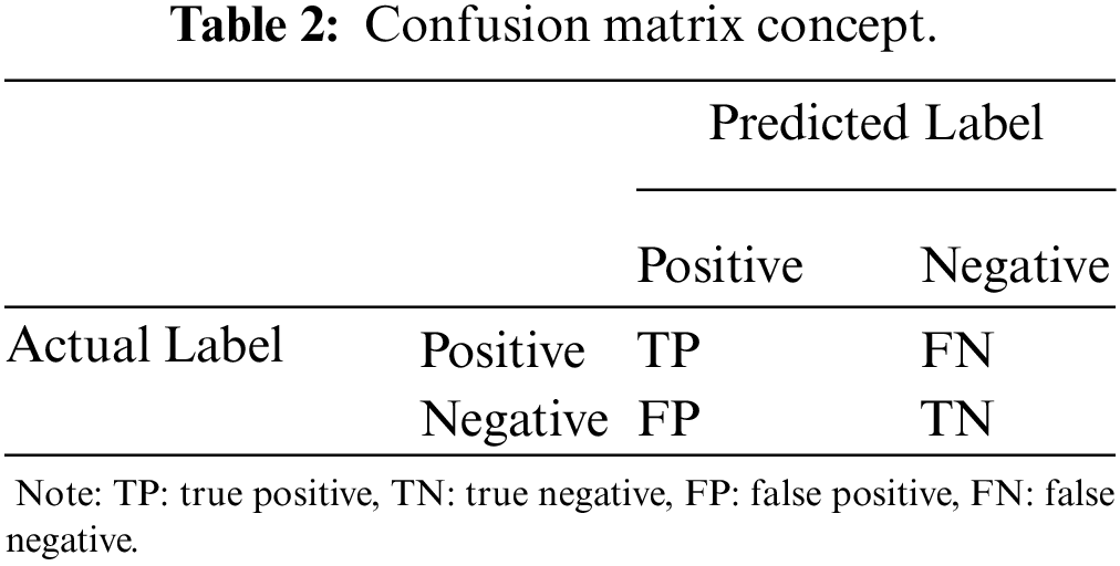
Nine CNN evaluation metrics were used to evaluate the CNN model, including training accuracy, p-value, test accuracy, AUC, sensitivity, precision, specificity, F1-score, and kappa. The concept of CNN evaluation metrics can be derived from the confusion matrix for binary classification, as shown in Tab. 2.

Where TP is a true positive, TN is a true negative, FP is a false positive, and FN is a false negative. From Tab. 2, the test accuracy (also known as overall accuracy (OA)), sensitivity, precision, specificity, F1-score, and kappa can be formulated as
OA=TP+TNTP+TN+FP+FN×100%,(1)
sensitivity=TPTP+FN,(2)
precision=TPTP+FP,(3)
specificity=TNTN+FP,(4)
F1−score=2⋅sensitivity⋅precisionsensitivity+precision,(5)
kappa=2(TP⋅TN−FN⋅FP)[(TP+FP)⋅(FP+TN)]+[(TP+FN)⋅(FN+TN)],(6)
while AUC can be expressed as a summary of the ROC curve [43,44].
4 Results and Discussions
The feature extraction method was run five times, corresponding to a specific fold, and the average values of accuracy and loss in training and validation were acquired. After 15 training with different optimizers, the results shown in the first row of Fig. 5 can be obtained. The feature extraction schemes with Adam, Adagrad, and SGD had similar conditions, offering low accuracy and high loss averages for the training and test datasets. Therefore, there is no optimal model for feature extraction. Subsequently, the fine-tuning technique with 25% was accomplished using the same scenario as the feature extraction. A total of 15 training procedures were performed to obtain the best model in this case, and the results are shown in the second row of Fig. 5. Adagrad with a 25% fine-tuning approach satisfied the criteria as the best model when compared with SGD with 25% fine-tuning, which provided overfitting identified from the loss average between training and validation, while Adam with 25% fine-tuning showed unsatisfactory training loss at almost 400% when the epoch was 150. Similarly, the model was trained using the same conditions and hyperparameters for a 75% fine-tuning procedure, and the results are shown in the third row of Fig. 5. Again, Adagrad with 75% fine-tuning provided the maximum accuracy average along with the minimum loss average, corresponding to training and validation. Nevertheless, SGD 75% and Adam 75% fine-tuning provided several uncertainties by showing validation loss fluctuations, leading to overfitting. The validation loss for Adam 75% reached almost 400% around the epoch of 120. To complete the entire 60 training procedures, the last 15 training procedures with a 100% fine-tuning scheme were conducted using the same preparation as the feature extraction, 25%, and 75% fine-tuning methods. The results are shown in the fourth row of Fig. 5. Adagrad 100% fine-tuning was superior, demonstrating sufficient accuracy and loss averages. The validation loss was roughly 5% and the training loss was approximately 0%. In addition, SGD 100% agreed with Adagrad 100% by presenting adequate accuracy and loss. The validation loss is less than 10%, whereas the training loss is approximately 0%. Evidently, Adam was not appropriate for any fine-tuning technique in this study, even Adam with 100% fine-tuning presented uncertainties in all epochs. To achieve a better illustration, Fig. 6 depicts the mean training accuracy with the standard deviation for the four best CNN models with Adagrad 25%, Adagrad 75%, Adagrad 100%, and SGD 100% fine-tuning. As depicted in Fig. 6, the mean accuracy increased following the level of fine-tuning in the last several layers in the CNN model. In contrast, the standard deviation decreased following the fine-tuning level.

Figure 5: Accuracy and loss average of 5-fold cross-validation for training and validation datasets. The first column is for Adagrad, the second column is for SGD, and the third column is for Adam. Additionally, the first row is for feature extraction, the second row is for 25% fine-tuning, the third row is for 75% fine-tuning, and the fourth row is for 100% fine-tuning. The red line is training accuracy, the blue line is validation accuracy, the green line is training loss, and the black line is validation loss. Adagrad: adaptive gradient optimizer, SGD: stochastic gradient descent, Adam: adaptive moment estimation

Figure 6: Mean training accuracy with the standard deviation for the four best CNN models with Adagrad 25%, Adagrad 75%, Adagrad 100%, and SGD 100% fine-tunings. CNN: convolutional neural network
By completing the entire model training procedure, we obtained the four best models involving the Adagrad 25%, 75%, 100%, and SGD 100% fine-tuning approaches. The following step was to evaluate the four best models using CNN metric evaluations, including p-value, test accuracy, AUC, sensitivity, precision, specificity, F1-score, and kappa. Fig. 7 depicts the confusion matrix of the four best models with TP=1170, TN=1403, FP=29, and FN=24 for Adagrad with 25% fine-tuning, as shown in Fig. 7a, meanwhile, TP=1180, TN=1415, FP=17, and FN=14 for Adagrad with 75% fine-tuning, as shown in Fig. 7b. Additionally, TP=1191, TN=1429, FP=3, and FN=3 for Adagrad with 100% fine-tuning, as shown in Fig. 7c, whereas TP=1194, TN=1431, FP=1, and FN=0 for SGD with 100% fine-tuning, as shown in Fig. 7d.

Figure 7: Confusion matrix for the four best CNN models with (a) Adagrad 25%, (b) Adagrad 75%, (c) Adagrad 100%, and (d) SGD 100% fine-tunings
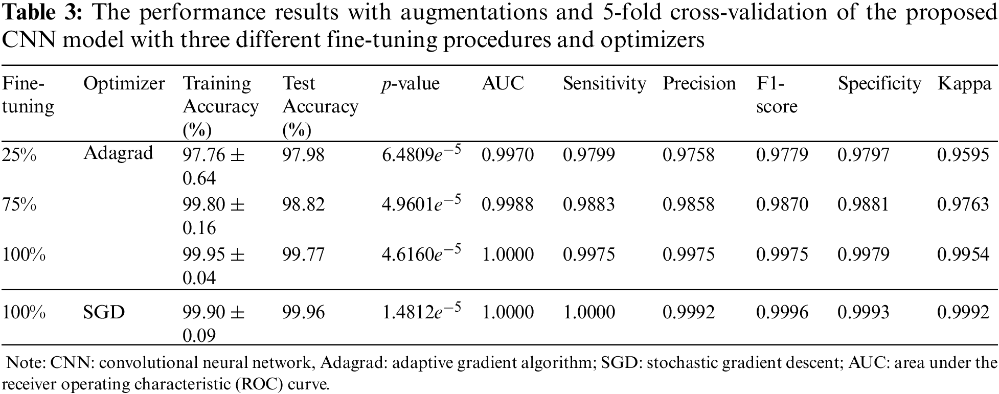
The results are summarized in Tab. 3. The training accuracy was in the range of 97.76%±0.64% to 99.95%±0.04% with p-value of 6.4809e−5 to 1.4812e−5 calculated from the improvement of training accuracy using fine-tuning versus feature extraction, while the test accuracy was in the range of 97.98% to 99.96%. Moreover, the AUC was 0.9970−1.0000, sensitivity was 0.9799−1.0000, precision was 0.9758−0.9992, F1-score was 0.9779−0.9996, specificity was 0.9797−0.9993, and kappa was 0.9595−0.9992. Compared to [36], in terms of sensitivity, specificity, F1-score, accuracy, and AUC, as shown in Tab. 1, our results showed 2%−6% enhancements. Our CNN best model results indicated that from the metric evaluations, with a more fine-tuning depth level, better results were obtained. Therefore, a fine-tuning method, along with data augmentation and 5-fold cross-validation, has a significant impact on the improvement of the proposed modified ResNet50 architecture in classifying breast masses corresponding to benign and malignant cancers. However, the improvement needs to be concentrated in the future related to the computation time and method to select the appropriate hyperparameters to increase efficiency.

5 Conclusions
The modified ResNet50, along with 5-fold cross-validation, data augmentations, and fine-tuning schemes, has been designed to classify breast masses related to benign and malignant cancers. In addition, this study employed the DDSM dataset collected from Mendeley data, which can be publicly accessed. To balance the dataset between benign and malignant, five data augmentations were allocated, namely color jitter, gamma correction, horizontal flip, salt and pepper, and sharpening. To increase the number of training datasets in each fold in the 5-fold, two image augmentations were assigned with random rotation up to 90∘ and a height shift of 0.3. Using the arrangement of 25%, 75%, and 100% fine-tunings, feature extraction, and three optimizers (Adam, Adagrad, and SGD), 12 models were obtained. By selecting the best accuracy and loss averages that did not comprise overfitting, four models were defined as the best model consisting of Adagrad 25%, 75%, 100%, and SGD 100% fine-tunings. Our AUC was in the range of 0.9970 to 1.0000 with a test accuracy of 97.98% to 99.96%. The results of nine CNN metric evaluations indicate that the optimized classifier is feasible for categorizing breast cancer as benign and malignant from the mammographic breast masses images. However, in a future study, optimization of the computational time is essential because, for every training, the time consumption was approximately 3.7 hours. Additionally, a method to select appropriate hyperparameters to increase efficiency is crucial.
Funding Statement: This research was supported by the National Research Foundation of Korea (NRF) grant funded by the Korean government (MSIT) [NRF-2019R1F1A1062397, NRF-2021R1F1A1059665] and Brain Korea 21 FOUR Project (Dept. of IT Convergence Engineering, Kumoh National Institute of Technology). This paper was supported by Korea Institute for Advancement of Technology (KIAT) grant funded by the Korea Government (MOTIE) [P0017123, The Competency Development Program for Industry Specialist].
Conflicts of Interest: The authors declare that they have no conflicts of interest to report regarding the present study.
References
1. Z. Xu, Z. Wang, J. Li, T. Jin, X. Meng et al., “Dendritic neuron model trained by information feedback-enhanced differential evolution algorithm for classification,” Knowledge-Based Systems, vol. 233, no. 7553, pp. 107536, 2021. [Google Scholar]
2. K. Fukushima, “Cognitron: A self-organizing multilayered neural network,” Biological Cybernetics, vol. 20, no. 3–4, pp. 121–136, 1975. [Google Scholar]
3. K. Fukushima, “Neocognitron: A self-organizing neural network model for a mechanism of pattern recognition unaffected by shift in position,” Biological Cybernetics, vol. 36, no. 4, pp. 193–202, 1980. [Google Scholar]
4. H. Singh, R. K. Sharma and V. P. Singh, “Online handwriting recognition systems for Indic and non-Indic scripts: A review,” Artificial Intelligence Review, vol. 54, no. 2, pp. 1525–1579, 2021. [Google Scholar]
5. Y. LeCun, L. D. Jackel, B. Boser, J. S. Denker, H. P. Graf et al., “Handwritten digit recognition: Applications of neural network chips and automatic learning,” IEEE Communications Magazine, vol. 27, no. 11, pp. 41–46, 1989. [Google Scholar]
6. B. M. Al-Helali and S. A. Mahmoud, “Arabic online handwriting recognition (AOHRA survey,” ACM Computing Surveys, vol. 50, no. 3, pp. 1–35, 2018. [Google Scholar]
7. R. Maalej and M. Kherallah, “Improving the DBLSTM for on-line Arabic handwriting recognition,” Multimedia Tools and Applications, vol. 79, no. 25-26, pp. 17969–17990, 2020. [Google Scholar]
8. A. Baldominos, Y. Saez and P. Isasi, “A survey of handwritten character recognition with MNIST and EMNIST,” Applied Sciences, vol. 9, no. 15, pp. 3169, 2019. [Google Scholar]
9. C. Y. Wu, S.-C. B. Lo, M. T. Freedman, A. Hasegawa, A. R. Zuurbier et al., “Classification of microcalcifications in radiographs of pathological specimen for the diagnosis of breast cancer,” Academic Radiology, vol. 2, no. 3, pp. 199–204, 1995. [Google Scholar]
10. M. A. Morid, A. Borjali and G. D. Fiol, “A scoping review of transfer learning research on medical image analysis using ImageNet,” Computers in Biology and Medicine, vol. 128, pp. 104115, 2021. [Google Scholar]
11. O. Russakovsky, J. Deng, H. Su, J. Krause, S. Satheesh et al., “ImageNet large scale visual recognition challenge,” International Journal of Computer Vision, vol. 115, no. 3, pp. 211–252, 2015. [Google Scholar]
12. A. Krizhevsky, I. Sutskever and G. E. Hinton, “ImageNet classification with deep convolutional neural networks,” Communications of the ACM, vol. 60, no. 6, pp. 84–90, 2017. [Google Scholar]
13. K. He, X. Zhang, S. Ren and J. Sun, “Deep residual learning for image recognition,” in Proc. of the IEEE Conf. on Computer Vision and Pattern Recognition (CVPR), Las Vegas, NV, USA, pp. 770–778, 2016. [Google Scholar]
14. M. Heath, K. Bowyer, D. Kopans, R. Moore and P. Kegelmeyer, “The digital database for screening mammography,” in Proc. of the Fifth Int. Workshop on Digital Mammography, M. J. Yaffe (ed.Toronto: Medical Physics Publishing, pp. 212–218, 2001. [Google Scholar]
15. D. Muduli, R. Dash and B. Majhi, “Automated breast cancer detection in digital mammograms: A moth flame optimization based ELM approach,” Biomedical Signal Processing and Control, vol. 59, no. 6, pp. 101912, 2020. [Google Scholar]
16. V. K. Singh, H. A. Rashwan, S. Romani, F. Akram, N. Pandey et al., “Breast tumor segmentation and shape classification in mammograms using generative adversarial and convolutional neural network,” Expert Systems with Applications, vol. 139, no. 12, pp. 112855, 2020. [Google Scholar]
17. I. C. Moreira, I. Amaral, I. Domingues, A. Cardoso, J. Cardoso et al., “INbreast: Toward a full-field digital mammographic database,” Academic Radiology, vol. 19, no. 2, pp. 236–248, 2012. [Google Scholar]
18. J. Suckling, J. Parker, D. Dance, S. Astley, I. Hutt et al., “Mammographic Image Analysis Society (MIAS) database v1.21 [Dataset],” 2015. [Online]. Available: https://www.repository.cam.ac.uk/handle/1810/250394. [Google Scholar]
19. R. Agarwal, O. Diaz, X. Lladó, M. H. Yap and R. Martí, “Automatic mass detection in mammograms using deep convolutional neural networks,” Journal of Medical Imaging, vol. 6, no. 3, pp. 031409, 2019. [Google Scholar]
20. C. Muramatsu, M. Nishio, T. Goto, M. Oiwa, T. Morita et al., “Improving breast mass classification by shared data with domain transformation using a generative adversarial network,” Computers in Biology and Medicine, vol. 119, pp. 103698, 2020. [Google Scholar]
21. W. M. Salama, A. M. Elbagoury and M. H. Aly, “Novel breast cancer classification framework based on deep learning,” IET Image Processing, vol. 14, no. 13, pp. 3254–3259, 2020. [Google Scholar]
22. H. Soleimani and O. V. Michailovich, “On segmentation of pectoral muscle in digital mammograms by means of deep learning,” IEEE Access, vol. 8, pp. 204173–204182, 2020. [Google Scholar]
23. M. A. Al-antari, S.-M. Han and T.-S. Kim, “Evaluation of deep learning detection and classification towards computer-aided diagnosis of breast lesions in digital X-ray mammograms,” Computer Methods and Programs in Biomedicine, vol. 196, pp. 105584, 2020. [Google Scholar]
24. B. Wei, Z. Han, X. He and Y. Yin, “Deep learning model based breast cancer histopathological image classification,” in Proc. of the IEEE 2nd Int. Conf. on Cloud Computing and Big Data Analysis (ICCCBDA), Chengdu, China, pp. 348–353, 2017. [Google Scholar]
25. K. Yu, L. Tan, L. Lin, X. Cheng, Z. Yi et al., “Deep-learning-empowered breast cancer auxiliary diagnosis for 5GB remote E-health,” IEEE Wireless Communications, vol. 28, no. 3, pp. 54–61, 2021. [Google Scholar]
26. E. Deniz, A. Şengür, Z. Kadiroğlu, Y. Guo, V. Bajaj et al., “Transfer learning based histopathologic image classification for breast cancer detection,” Health Information Science and Systems, vol. 6, no. 1, pp. 18, 2018. [Google Scholar]
27. H. Chougrad, H. Zouaki and O. Alheyane, “Deep convolutional neural networks for breast cancer screening,” Computer Methods and Programs in Biomedicine, vol. 157, no. 2017, pp. 19–30, 2018. [Google Scholar]
28. L. Zhang, A. A. Mohamed, R. Chai, Y. Guo, B. Zheng et al., “Automated deep learning method for whole-breast segmentation in diffusion-weighted breast MRI,” Journal of Magnetic Resonance Imaging, vol. 51, no. 2, pp. 635–643, 2020. [Google Scholar]
29. S. S. Aboutalib, A. A. Mohamed, W. A. Berg, M. L. Zuley, J. H. Sumkin et al., “Deep learning to distinguish recalled but benign mammography images in breast cancer screening,” Clinical Cancer Research, vol. 24, no. 23, pp. 5902–5909, 2018. [Google Scholar]
30. R. L. Siegel, K. D. Miller and A. Jemal, “Cancer statistics,” CA: A Cancer Journal for Clinicians, vol. 69, no. 1, pp. 7–34, 2019. [Google Scholar]
31. R. K. Samala, H.-P. Chan, L. M. Hadjiiski, M. A. Helvie, K. H. Cha et al., “Multi-task transfer learning deep convolutional neural network: Application to computer-aided diagnosis of breast cancer on mammograms,” Physics in Medicine & Biology, vol. 62, no. 23, pp. 8894–8908, 2017. [Google Scholar]
32. D. Saranyaraj, M. Manikandan and S. Maheswari, “A deep convolutional neural network for the early detection of breast carcinoma with respect to hyper- parameter tuning,” Multimedia Tools and Applications, vol. 79, no. 15-16, pp. 11013–11038, 2020. [Google Scholar]
33. H. Yang and F. Wang, “Wireless network intrusion detection based on improved convolutional neural network,” IEEE Access, vol. 7, pp. 64366–64374, 2019. [Google Scholar]
34. L. Sun, J. Wang, Z. Hu, Y. Xu and Z. Cui, “Multi-view convolutional neural networks for mammographic image classification,” IEEE Access, vol. 7, pp. 126273–126282, 2019. [Google Scholar]
35. H. N. Khan, A. R. Shahid, B. Raza, A. H. Dar and H. Alquhayz, “Multi-view feature fusion based four views model for mammogram classification using convolutional neural network,” IEEE Access, vol. 7, pp. 165724–165733, 2019. [Google Scholar]
36. S. J. Malebary and A. Hashmi, “Automated breast mass classification system using deep learning and ensemble learning in digital mammogram,” IEEE Access, vol. 9, pp. 55312–55328, 2021. [Google Scholar]
37. H. Li, D. Chen, W. H. Nailon, M. E. Davies and D. I. Laurenson, “Dual convolutional neural networks for breast mass segmentation and diagnosis in mammography,” IEEE Transactions on Medical Imaging, vol. 41, no. 1, pp. 3–13, 2022. [Google Scholar]
38. E. J. Kendall, M. G. Barnett and K. Chytyk-Praznik, “Automatic detection of anomalies in screening mammograms,” BMC Medical Imaging, vol. 13, no. 1, pp. 43, 2013. [Google Scholar]
39. M.-L. Huang and T.-Y. Lin, “Dataset of breast mammography images with masses,” Data in Brief, vol. 31, no. 2, pp. 105928, 2020. [Google Scholar]
40. X. Zhang, J. Zhou, W. Sun and S. K. Jha, “A lightweight CNN based on transfer learning for COVID-19 diagnosis,” Computers Materials & Continua, vol. 72, no. 1, pp. 1123–1137, 2022. [Google Scholar]
41. G. Ayana, J. Park and S.-W. Choe, “Patchless multi-stage transfer learning for improved mammographic breast mass classification,” Cancers, vol. 14, no. 5, pp. 1280, 2022. [Google Scholar]
42. S. Muthukumarasamy, A. K. Tamilarasan, J. Ayeelyan and M. A., “Machine learning in healthcare diagnosis,” Blockchain and Machine Learning for e-Healthcare Systems, London, United Kingdom: IET-Institution of Engineering and Technology, vol. 14, pp. 343–366, 2020. [Google Scholar]
43. A. E. Maxwell, T. A. Warner and L. A. Guillén, “Accuracy assessment in convolutional neural network-based deep learning remote sensing studies—Part 1: Literature review,” Remote Sensing, vol. 13, no. 13, pp. 2450, 2021. [Google Scholar]
44. S. Vijayalakshmi, A. John, R. Sunder, S. Mohan, S. Bhattacharya et al., “Multi-modal prediction of breast cancer using particle swarm optimization with non-dominating sorting,” International Journal of Distributed Sensor Networks, vol. 16, no. 11, pp. 1–12, 2020. [Google Scholar]