Computers, Materials & Continua DOI:10.32604/cmc.2022.031247
Article

Hyperparameter Tuning Bidirectional Gated Recurrent Unit Model for Oral Cancer Classification

K. Shankar1, E. Laxmi Lydia2, Sachin Kumar1,*, Ali S. Abosinne3, Ahmed alkhayyat4, A. H. Abbas5 and Sarmad Nozad Mahmood6

1Department of Computer Science, South Ural State University, Chelyabinsk, 454080, Russia
2Department of Computer Science and Engineering, Vignan’s Institute of Information Technology, Visakhapatnam, 530049, India
3Computer Technical Engineering Department, College of Technical Engineering, the Islamic University, Najaf, 54001, Iraq
4College of Technical Engineering, the Islamic University, Najaf, Iraq
5College of Information Technology, Imam Ja’afar Al-Sadiq University, Al-Muthanna, 66002, Iraq
6Computer Technology Engineering, College of Engineering Technology, Al-Kitab University, Iraq
*Corresponding Author: Sachin Kumar. Email: sachinagnihotri16@gmail.com
Received: 13 April 2022; Accepted: 25 May 2022

Abstract: Oral Squamous Cell Carcinoma (OSCC) is a type of Head and Neck Squamous Cell Carcinoma (HNSCC) and it should be diagnosed at early stages to accomplish efficient treatment, increase the survival rate, and reduce death rate. Histopathological imaging is a wide-spread standard used for OSCC detection. However, it is a cumbersome process and demands expert’s knowledge. So, there is a need exists for automated detection of OSCC using Artificial Intelligence (AI) and Computer Vision (CV) technologies. In this background, the current research article introduces Improved Slime Mould Algorithm with Artificial Intelligence Driven Oral Cancer Classification (ISMA-AIOCC) model on Histopathological images (HIs). The presented ISMA-AIOCC model is aimed at identification and categorization of oral cancer using HIs. At the initial stage, linear smoothing filter is applied to eradicate the noise from images. Besides, MobileNet model is employed to generate a useful set of feature vectors. Then, Bidirectional Gated Recurrent Unit (BGRU) model is exploited for classification process. At the end, ISMA algorithm is utilized to fine tune the parameters involved in BGRU model. Moreover, ISMA algorithm is created by integrating traditional SMA and Chaotic Oppositional Based Learning (COBL). The proposed ISMA-AIOCC model was validated for performance using benchmark dataset and the results pointed out the supremacy of ISMA-AIOCC model over other recent approaches.

Keywords: Computer aided diagnosis; deep learning; BGRU; biomedical imaging; oral cancer; histopathological images

1  Introduction

The studies conducted upon cancer analysis have increased in the past few years. In order to diagnose the presence and classify the type and phase of cancer, scientific scholars have developed distinct screening methodologies for initial phase diagnosis [1]. With the arrival of new technologies, huge volumes of cancer information are being collected which can be accessed by the medical research group [2]. However, the most difficult task for medical fraternity is to estimate the kinds of cancer in a precise manner. Oral Squamous Cell Carcinoma (OSCC) is a heterogeneous class of cancer that affects the mucosal lining of oral cavity and is responsible for more than 90% of oral malignancies [3,4]. Early prognosis of OSCC is important for efficacious treatment, increased survival chances, and reduction in decease and morbidity rates. However, OSCC recorded the worst diagnosis rate with a 50% total endurance rate so far [5]. Recently, microscopy-related histopathological examination of tissue biopsies has been decided as the golden standard for prognosis of OSCC. This pathology-based diagnostic technique depends on histopathologists. So, the process is not only time-consuming one, but also prone to human and medical errors in making decisions. These drawbacks restrict the application of results in clinical decisions [6]. So it has become necessary to enhance the effectiveness of diagnostic instruments which will be helpful in guiding the pathologists in prognosis as well as interpretation process of OSCC. Thus, various Machine Learning (ML) methods are utilized by medical researchers. Such methods are highly efficient in finding the patterns and relationships between the patterns. They tend to effectively estimate the upcoming results i.e., cancer type from complex datasets.

Oncologists provide the prognosis to patients based on the records presented by pathologists. In this scenario, these records should be precise, informative and kept with high confidentiality since it holds highly important information [7]. Hence, the whole manual functions like considering every portion of the slide and interpreting the features are time taking and it also requires experienced professionals. In addition to this, the records may also experience observer bias [8]. In such problems, a mechanized system of the previously-mentioned processes can minimize the bias as well as time, thereby increasing the precision of interpretation of the characteristics. So, a Computer Aided Diagnostic (CAD) system for oral cancer prognosis is the need of the hour, especially in a resource-constraint and developing country like India. This system will be useful for labs that handle huge loads of data on a daily basis. Further, in general cancer awareness camps, large number of cases are diagnosed as normal. Due to this, pathologists can focus on cases diagnosed by the system as malicious [9]. Currently, there is an increasing corpus of studies being conducted on enhancing medical prognosis by utilizing Artificial Intelligence (AI). The rise in the usage of diagnostic imaging allows the researchers to deploy AI applications in the interpretation of medical images [10].

Bashir et al. [11] presented a new morphometric method to exploit the structural feature from dysplastic lesions. In other terms, irregular epithelial stratification can be measured for the widths of distinct layers of epithelium in boundary layer. Further, keratin projecting in basal and epithelium layers should also be investigated for resting tissue section in a clinically-important view. Rashid et al. [12] proposed Multi-scale Dilated U-Net (MD-UNet) that carries out feature extraction at several scales and describes accurate boundary. The proposed MD-UNet was trained using five Nuclei Segmentation datasets all of which are appropriate to distinct organs of human body.

The authors in the literature [13] presented a Deep Learning (DL)-based structure that detects oral cancer using histopathology images in a highly effective manner. In this method, the color channel was split, deep features were extracted and categorized under individual channels instead of single integrated channel using EfficientNetB3. This feature was fused from various channels with the help of feature fusion element, planned as a layer, and located before the dense layer of EfficientNetB3. Silva et al. [14] examined a dysplasia quantification approach using ML techniques in which histopathological images of oral cavity were used. This technique contains nuclei segmentation stages, feature extraction, classification, and post-processing. During segmentation stage, mask region-based Convolution Neural Network (R-CNN) was trained to utilize nuclei masks in which an object is identified. The authors [15] presented a deep dictionary learning technique to resolve tissue phenotyping issue from histopathology images. This study presented a deep Multi-Resolution Dictionary Learning (deepMRDL) model and used deep texture descriptors at several distinct spatial resolutions.

The current research article introduces Improved Slime Mould Algorithm with Artificial Intelligence Driven Oral Cancer Classification (ISMA-AIOCC) model to be used in histopathological images. The presented ISMA-AIOCC model uses linear smoothing filter to remove the noise. Besides, MobileNet model is employed to generate a useful set of feature vectors. Then, Bidirectional Gated Recurrent Unit (BGRU) model is exploited for classification process. Finally, ISMA algorithm is utilized to fine tune the parameters involved in BGRU model. The performance validation of ISMA-AIOCC model was conducted upon benchmark dataset and the results were measured under distinct measures.

2  The Proposed Model

In this study, a new ISMA-AIOCC model has been developed for identification and categorization of oral cancer using HIs. At initial stage, linear smoothing filter is applied to remove the noise. Moreover, MobileNet model is employed to generate a useful set of feature vectors. Furthermore, ISMA-BGRU model is exploited for classification process. Fig. 1 illustrates the overall process involved in ISMA-AIOCC technique.

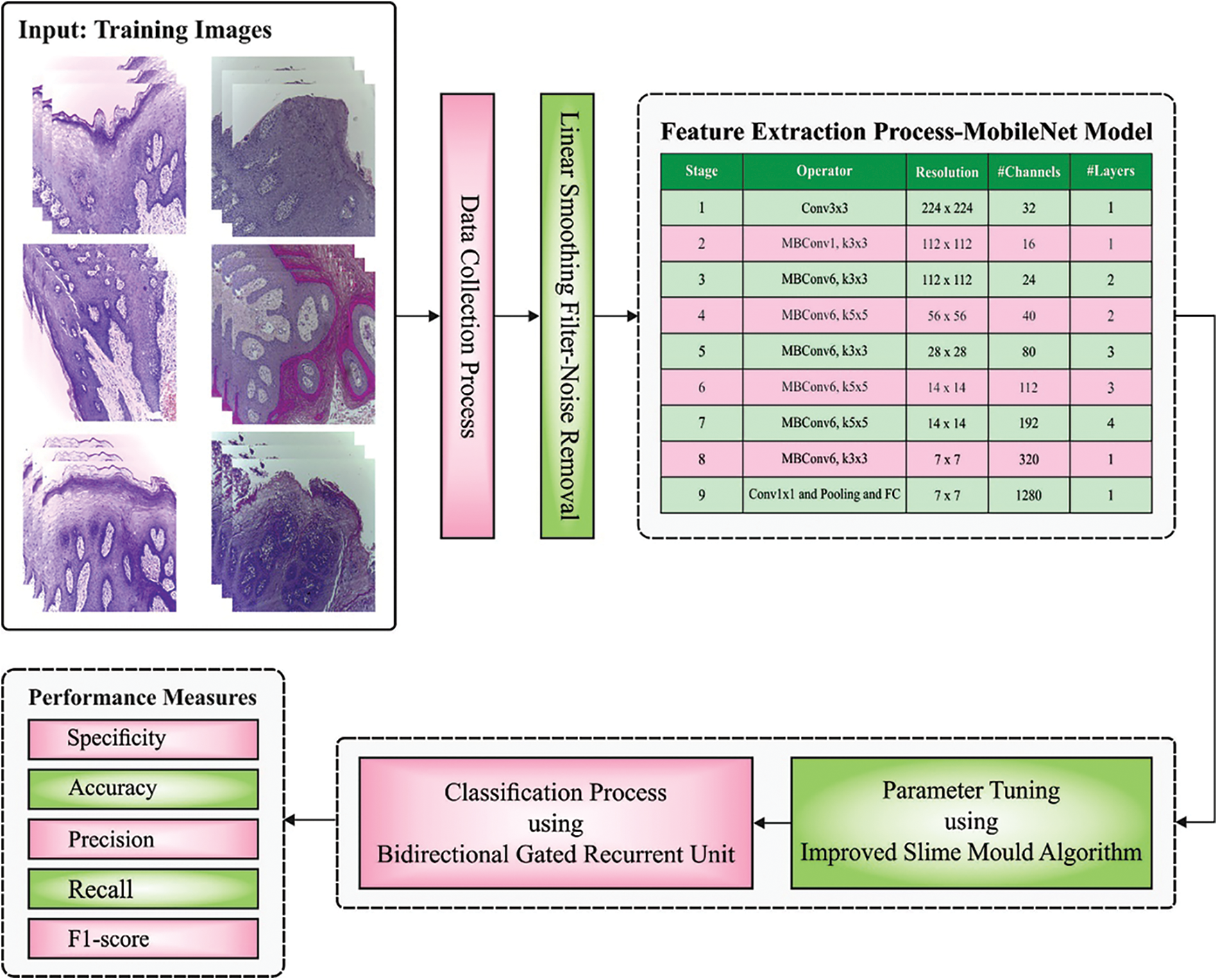
Figure 1: Overall process of ISMA-AIOCC technique

2.1 Image Filtering Approach

Initially, linear smoothing filter is applied to remove the noise. Linear or Mean filtering operates by a pixel through the reduction of sum of intensity variations between single and the following pixels. Each pixel value in the image is interchanged with mean (`average’) value of each neighbour [16]. This filtering process removes the pixel value that is unrepresentative or dissimilar to the nearby pixel. Consider Sxv characterizes the set of coordinates in a rectangular sub-image window sized X b and use the pixel at the centre represented by (x, y). The filtering procedure calculates the average value of image g(x, y) in rectangular region which is determined using Sxy. The values of the image at point (x, y) represent arithmetical mean value, calculated by the pixel, in the region determined as S. In other words, it is given as follows.

f(x,y)=1ab∑(s,t)∈Sx,yg(s,t)(1)

2.2 Feature Extraction: MobileNet Model

After data preprocessing, MobileNet model is employed to generate a useful set of feature vectors. MobileNet [17] is a framework which is aimed at running on embedded and mobile devices or systems that lack computation power. This structural design was projected by Google. Depth-wise separable convolutional layer is utilized in MobileNet framework to drastically reduce the amount of trained variables in comparison with standard Convolution Neural Network (CNN) which has similar depth. Depth-wise separable convolutional layer handles both depth as well as spatial dimensions. Depth-wise separable convolutional layer separates the kernel into two smaller kernels namely, pointwise and depthwise-convolutional layers. The separation of kernel decreases the computation cost considerably. MobileNet provides outcomes that are compared to AlexNet, when decreasing the trained variables significantly. In this work, a pretrained MobileNet architecture is introduced. Then, a dense layer of 128 × 1 replaces the classifier portion of architecture i.e., 3 × 1 and 128 × 1, 2 × 1 for binary and ternary classifications, correspondingly. At the time of fine-tuning process, MobileNetV2 provides an input image of 224 × 224 × 3 dimensions. Then, the input experiences pointwise and depth-wise convolutional layers, multiple times. Finally, the feature attained from the above-mentioned procedure is given into two dense layers of 128 × 1 and 3 × 1 or 2 × 1 dimensions for classifier tasks. The abovementioned procedure is iterated for numerous times in backward and forward propagations through Adam optimizer.

2.3 Image Classification: BGRU Model

For effective identification of class labels, the features are then fed into BGRU model [18]. Recurrent Neural Networks (RNN) have a strong ability to handle context-dependent sequences. But, it is challenging to train RNN because of gradient vanishing problem. Recently, Recurrent Neural Network (RNN) with gated units, for example, Gated Recurrent Unit (GRU) and Long Short Term Memory (LSTM) have become popular since both are effective in nature. Here, GRU is utilized for capturing the global context, since it accomplishes comparative outcomes with lesser parameters than LSTM. The equations for GRU algorithm are given below.

rt=sigm(Wlr⋅lt+Whr⋅ht−1+br),(2)

ut=sigm(Wlu⋅lt+Whu⋅ht−1+bu),(3)

h~t=tanh(Wlh~⋅lt+Whh~⋅(rt⊙ht−1+bh~),(4)

ht=ut⊙ht−1+(1−ut)⊙h~t,(5)

Whereas ht(∈Rk),rt,ut,h~t, denote the activation of internal memory cell, reset gate, update gate, and GRU output correspondingly, when the number of hidden layers is; br,bu,bh~(∈Rk) represent bias terms and k; Wlr,Whr,Wlu,Whu,Wlh~,Whh~(∈R3q×k) indicate the weight matrix. Furthermore, tanh⊙, and sigm indicate hyperbolic, element-wise multiplication, and sigmoid functions, correspondingly. In comparison with LSTM that contains one output state, one external memory cell state, and three gates i.e., output, input, and forget gates, GRU contains one output state and two gates such as reset and update gates. LSTM does not have sufficient essential gates i.e., output gate. So, it collectively combines the input and forget gates to form the reset and update gates for controlling, while the data must be theatrically forgotten or remembered. In terms of comparison, the overall amount of variables in a GRU is 3/4 of the number in LSTM.

The study utilizes bidirectional GRU while all of them contain backward GRU (from t=T to t=0) and forward GRU (from t=0 to t=T). The output from backward and forward GRUs, at time t, are connected to form the output from Bi-directional GRU (BGRU) simultaneously. Fig. 2 depicts the framework of BGRU. Moreover, to improve the global data flow, three BGRUs are stacked together with dropout so as to enhance the efficiency of the network. It is to be noted that the forward hidden layer of stacked BGRU can be evaluated by hforward−tz=GRU(htz−1,hforward−t−1z), whereas z and htz−1 indicate layer index and the connected output of previous layer in stacked BGRU. Eventually, the attained local and global frameworks are together connected as input to the subsequent layer.

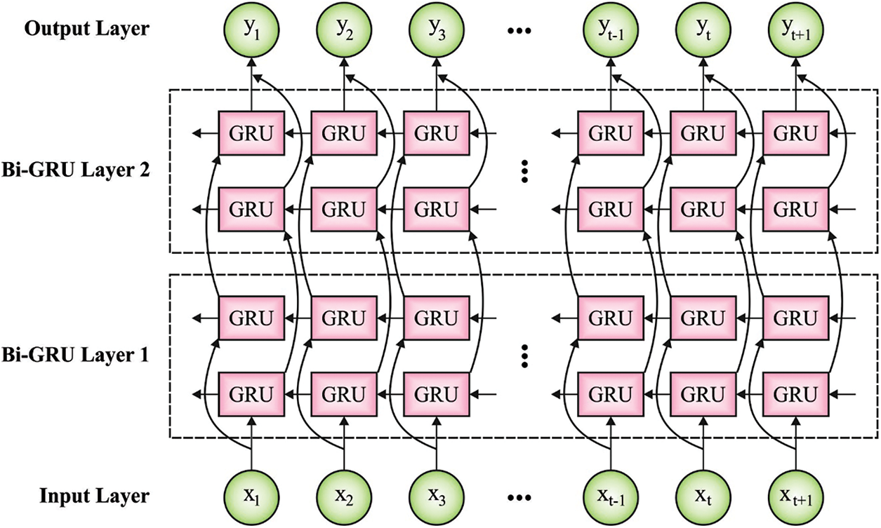
Figure 2: Structure of BGRU

2.4 Hyperparameter Optimization

In this final stage, ISMA algorithm is utilized to fine tune the parameters involved in BGRU. SMA works by simulating the morphological and behavioural changes of slime mould in foraging process. It can be mathematically expressed through the following equation [19]:

Xt+1={Xtbest+vb⋅(W⋅XtA−XtB)rand<p,νc⋅Xt′rand≥p,(6)

Here, t indicates the number of existing iterations. Xtbest represents the optimum individual. XtA and XtB signify two individuals that are chosen arbitrarily from the population in iteration t.νb denotes a variable that lies within −a to a.νc indicates a parameter which reduces from 1 to 0.W symbolizes the weight of slime mould. p indicates a parameter that is estimated as follows:

p=tanh|S(i)−DF|,i=1,2,3,…,NP,(7)

Now, S(i) indicates the fitness of X. NP represents the population count. DF denotes the optimal fitness value which are given in the following equation:

a=arctanh(−(ttmax)+1),(8)

Whereas tmax indicates the maximal amount of iterations.

W equation is evaluated as follows.

W(smellindex(i))={l+rand⋅log(bF−S(i)bF−ωF),conditionsl−rand⋅log(bF−S(i)bF−ωF),others,(9)

smellindex=sort(S),(10)

Here, the condition refers to individual ranking in the top half of fitness. bF and ωF denote the optimal fitness and worst fitness in the present population, correspondingly. It is mathematically given herewith.

Xt+1={rand⋅(ub−lb)+lb,rand<zXtbest+νb(WXtA′−XtB)rand<pvc⋅Xirand≥p(11)

In this equation, ub indicates the upper bound of searching space and ub represents the lower bounds of searching space, correspondingly.

Moreover, ISMA algorithm is created by integrating traditional SMA and COBL. Opposition-Based Learning (OBL) is a novel technology that has recently appeared in computing and was projected by Tizhoosh. According to this technique, there is a high likelihood that the reverse solution gets close to the global optimum solution than the original solution. OBL improves the diversity of the population by producing reverse location and evaluating both reverse and original individuals to maintain the predominant individual into the following generation. It is mathematically expressed as given in the following equation:

Xio=lb+ub−Xit,(12)

Here, Xio indicates the reverse solution that corresponds to Xit.

In order to overcome the deficiency and improve the population diversity, the reverse solution is produced by OBL. Though this solution is not exactly superior to the existing solution, it considers that chaotic mapping has ergodicity and randomness features. So, it can assist in generating new solutions and improve the diversity of the population. Consequently, it integrates both chaotic mapping and OBL and proposes a chaotic OBL approach. It is mathematically expressed through the following equation:

XiTo=lb+ub−λi⋅Xit.(13)

Now, XiTo signifies the inverse solution that corresponds to ith individual. λi represents the chaotic mapping value.

3  Results and Discussion

In this section, the experimental validation of the proposed ISMA-AIOCC model was conducted using two datasets [20] such as set-1 (100x) and set-2 (400x) datasets (https://data.mendeley.com/datasets/ftmp4cvtmb/1). Fig. 3 illustrates the sample images. The details related to the dataset are given in Tab. 1.

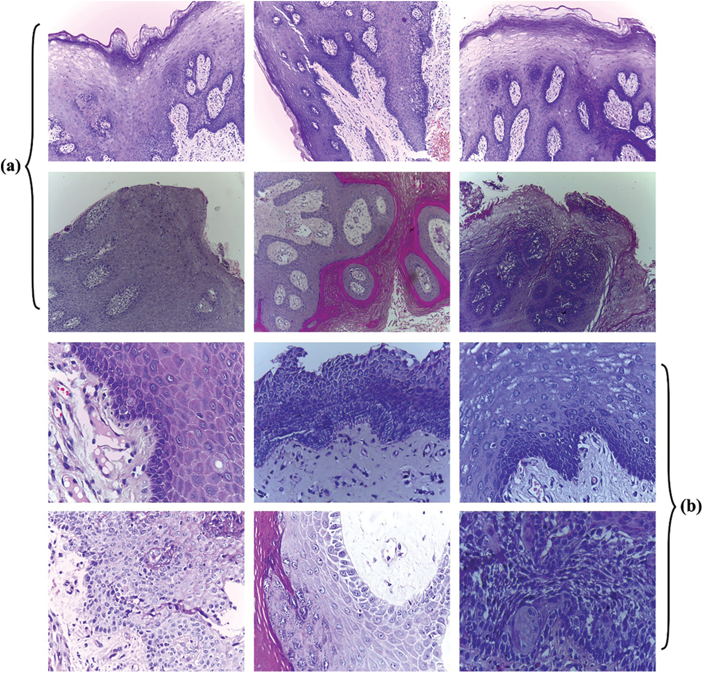
Figure 3: Sample Images (Normal/OSCC) a) Set-01 b) Set-02

Fig. 4 demonstrates the confusion matrices generated by ISMA-AIOCC model on distinct sizes of training (TR)/testing (TS) set-1. With 80% TR data, the proposed ISMA-AIOCC model classified 49 samples as normal class and 346 samples as OSCC class. Also, with 20% TS data, the presented ISMA-AIOCC method categorized 14 samples under normal class and 85 samples under OSCC class. At the same time, with 70% TR data, ISMA-AIOCC model recognized 48 samples as normal class and 309 samples as OSCC class. Moreover, with 30% TS data, the proposed ISMA-AIOCC system classified 31 samples as normal class and 126 samples as OSCC class.

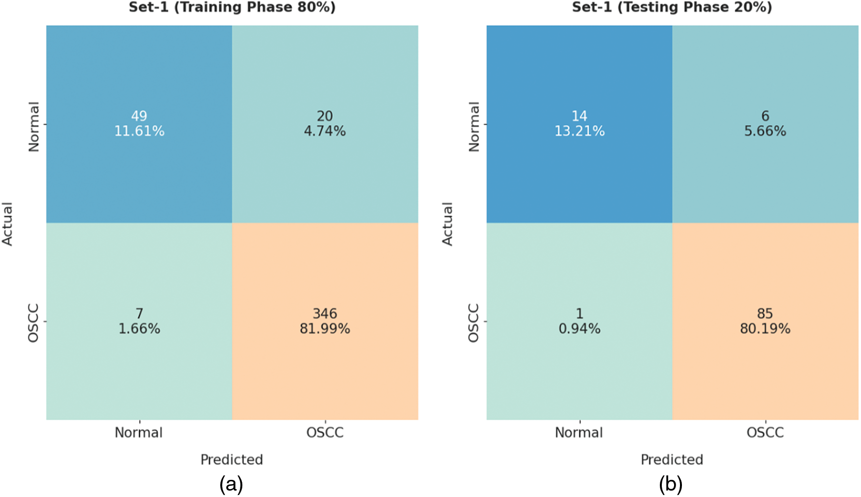
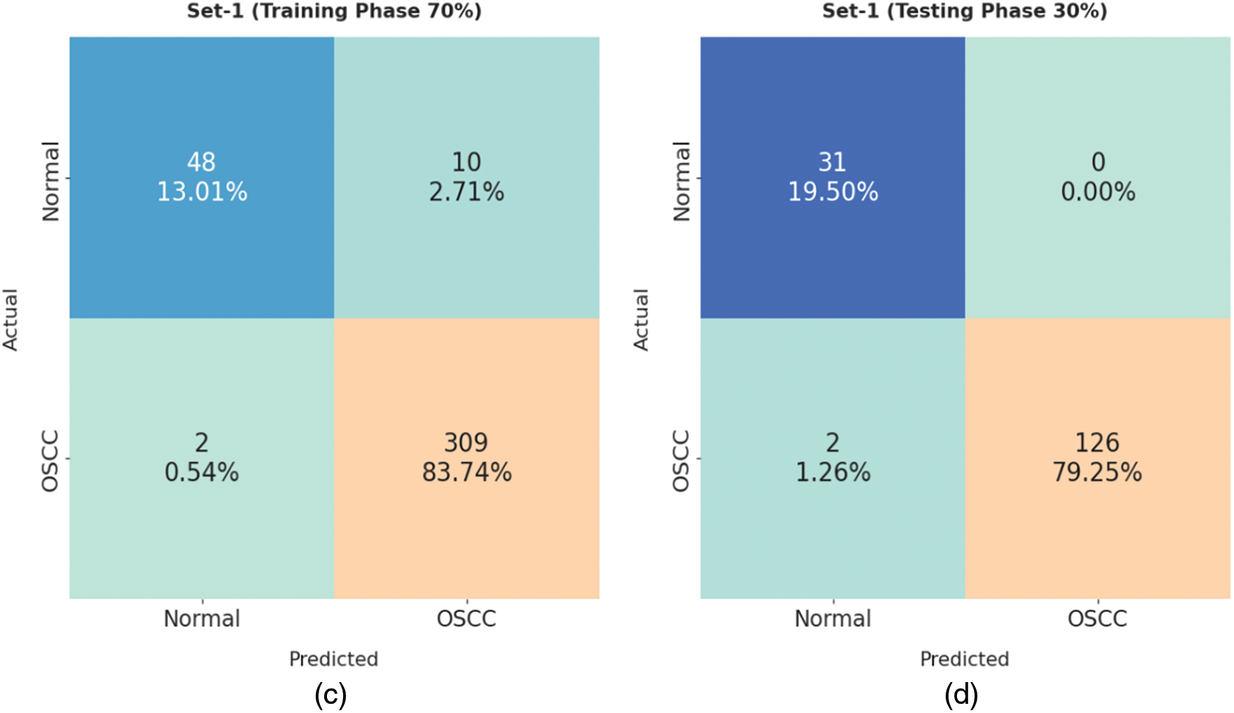
Figure 4: Confusion matrix of ISMA-AIOCC technique on set-1: a) 80% of TR, b) 20% of TS, c) 70% of TR, and d) 30% of TS

Tab. 2 and Fig. 5 provided a detailed illustration on OSCC classification outcome achieved by ISMA-AIOCC model on set-1 dataset. The obtained values indicate that ISMA-AIOCC model gained effectual outcomes under all classes. For instance, with 80% TR data, the proposed ISMA-AIOCC model achieved accuy, precn, recal, specy, and Fscore values such as 93.60%, 91.02%, 84.52%, 84.52%, and 87.32% respectively. Meanwhile, with 70% TR data, the proposed ISMA-AIOCC approach attained accuy, precn, recal, specy, and Fscore values such as 96.75%, 96.43%, 91.06%, 91.06%, and 93.49% correspondingly. Eventually, with 30% TS data, the presented ISMA-AIOCC algorithm accomplished accuy, precn, recal, specy, and Fscore values such as 98.74%, 96.97%, 99.22%, 99.22%, and 98.04% correspondingly.

Figure 5: Results of the analysis of ISMA-AIOCC technique on Set-1: a) 80% of TR, b) 20% of TS, c) 70% of TR, and d) 30% of TS

Fig. 6 demonstrate the Training Accuracy (TA) and Validation Accuracy (VA) values attained by ISMA-AIOCC model on set-1 dataset. The experimental outcomes imply that ISMA-AIOCC model gained maximum TA and VA values. To be specific, VA seemed to be higher than TA.

Figure 6: TA and VA analysis of ISMA-AIOCC approach on Set-1 dataset

Fig. 7 shows the Training Loss (TL) and Validation Loss (VL) values achieved by ISMA-AIOCC model on set-1 dataset. The experimental outcome infers that the proposed ISMA-AIOCC model accomplished the least values of TL and VL. To be specific, VL seemed to be lower than TL.

Figure 7: TL and VL analysis of ISMA-AIOCC approach on Set-1 dataset

Fig. 8 illustrates the confusion matrices generated by ISMA-AIOCC approach on distinct sizes of training/testing set-2. With 80% TR data, the proposed ISMA-AIOCC technique classified 125 samples as normal class and 392 samples as OSCC class. Also, with 20% TS data, the presented ISMA-AIOCC algorithm categorized 29 samples under normal class and 101 samples under OSCC class. Simultaneously, with 70% TR data, ISMA-AIOCC method recognized 132 samples as normal class and 343 samples as OSCC class. Furthermore, with 30% TS data, the proposed ISMA-AIOCC approach classified 54 samples as normal class and 150 samples as OSCC class.

Figure 8: Confusion matrix of ISMA-AIOCC technique on Set-2: a) 80% of TR, b) 20% of TS, c) 70% of TR, and d) 30% of TS

Tab. 3 and Fig. 9 demonstrate a detailed OSCC classification outcome accomplished by ISMA-AIOCC model on Set-2 dataset. The obtained values reveal that ISMA-AIOCC approach gained effectual outcomes under all classes. For instance, with 80% TR data, the proposed ISMA-AIOCC model achieved accuy, precn, recal, specy, and Fscore values such as 92.99%, 94.90%, 88.33%, 88.33%, and 90.88% respectively. In the meantime, with 70% TR data, the presented ISMA-AIOCC technique accomplished accuy, precn, recal, specy, and Fscore values such as 97.54%, 97.84%, 96.19%, 96.19%, and 96.97% correspondingly. At last, with 30% TS data, ISMA-AIOCC approach attained accuy, precn, recal, specy, and Fscore values such as 97.61%, 98.39%, 95.76%, 95.76%, and 96.97% correspondingly.

Figure 9: Results of the analysis of ISMA-AIOCC technique on Set-2: a) 80% of TR, b) 20% of TS, c) 70% of TR, and d) 30% of TS

Fig. 10 shows the TA and VA values achieved by ISMA-AIOCC model on Set-2 dataset. The experimental outcomes imply that ISMA-AIOCC approach gained maximum TA and VA values. To be specific, VA seemed to be higher than TA.

Figure 10: TA and VA analysis results of ISMA-AIOCC approach on Set-2 dataset

TL and VL values gained by the proposed ISMA-AIOCC model on Set-2 dataset are shown in Fig. 11. The experimental outcomes infer that the proposed ISMA-AIOCC technique accomplished the least TL and VL values. To be specific, VL seemed to be lower than TL.

Figure 11: TL and VL analysis results of ISMA-AIOCC approach on Set-2 dataset

In order to highlight the enhanced performance of ISMA-AIOCC technique, a comparison study was conducted and the results are shown in Fig. 12 [21]. The experimental results indicate that Visual Geometry Group (VGG16) and Support Vector Machine (SVM) models obtained the least classification performance. At the same time, Inception v3 and ResNet50 models produced slightly improved classifier results. Along with that, the Concatenated model and CNN models showcased reasonable performance over other methods. However, the proposed ISMA-AIOCC model surpassed all other techniques and achieved maximum accuy, precn, recal, F1score, and specy values such as 98.74%, 96.97%, 99.22%, 98.04%, and 99.22% respectively.

Figure 12: Comparative analysis of ISMA-AIOCC technique with existing approaches

By looking into the aforementioned tables and figures, it is clear that the proposed ISMA-AIOCC model accomplished the maximal classification performance over other methods.

4  Conclusion

In this study, a novel ISMA-AIOCC model has been developed for identification and categorization of oral cancer using HIs. At the initial stage, linear smoothing filter is applied to remove the noise from images. Besides, MobileNet model is employed to generate a useful set of feature vectors. Then, BGRU model is exploited for classification process. Finally, ISMA algorithm is utilized to fine tune the parameters involved in BGRU. Moreover, ISMA algorithm is derived by integrating traditional SMA and COBL. The performance validation of the proposed ISMA-AIOCC model was conducted using benchmark dataset and the outcomes confirmed the supremacy of ISMA-AIOCC model over recent approaches. In future, ISMA-AIOCC model can be tested using large scale datasets.

Funding Statement: The work is supported by the Ministry of Science and Higher Education of the Russian Federation (Government Order FENU-2020–0022).

Conflicts of Interest: The authors declare that they have no conflicts of interest to report regarding the present study.

References

1. S. Panigrahi and T. Swarnkar, “Machine learning techniques used for the histopathological image analysis of oral cancer-a review,” The Open Bioinformatics Journal, vol. 13, no. 1, pp. 106–118, 2020.
2. M. Fraz, S. A. Khurram, S. Graham, M. Shaban, M. Hassan et al. “FABnet: Feature attention-based network for simultaneous segmentation of microvessels and nerves in routine histology images of oral cancer,” Neural Computing and Applications, vol. 32, no. 14, pp. 9915–9928, 2019.
3. S. Panigrahi, J. Das and T. Swarnkar, “Capsule network based analysis of histopathological images of oral squamous cell carcinoma,” Journal of King Saud University-Computer and Information Sciences, pp. 1–8, 2020. https://doi.org/10.1016/j.jksuci.2020.11.003.
4. S. Sharma and R. Mehra, “Conventional machine learning and deep learning approach for multi-classification of breast cancer histopathology images—a comparative insight,” Journal of Digital Imaging, vol. 33, no. 3, pp. 632–654, 2020.
5. D. Komura and S. Ishikawa, “Machine learning methods for histopathological image analysis,” Computational and Structural Biotechnology Journal, vol. 16, pp. 34–42, 2018.
6. L. Ma, M. Halicek, X. Zhou, J. Dormer and B. Fei, “Hyperspectral microscopic imaging for automatic detection of head and neck squamous cell carcinoma using histologic image and machine learning,” in Medical Imaging 2020: Digital Pathology, Houston, Texas, United States, vol. 11320, pp. 113200W, 2020.
7. T. Y. Rahman, L. B. Mahanta, A. K. Das and J. D. Sarma, “Histopathological imaging database for oral cancer analysis,” Data in Brief, vol. 29, pp. 105114, 2020.
8. J. Gamper, B. Chan, Y. W. Tsang, D. Snead and N. Rajpoot, “Meta-svdd: Probabilistic meta-learning for one-class classification in cancer histology images,” arXiv preprint arXiv:2003.03109, 2020. https://doi.org/10.48550/arXiv.2003.03109.
9. A. Krishna, A. Tanveer, P. Bhagirath and A. Gannepalli, “Role of artificial intelligence in diagnostic oral pathology-A modern approach,” Journal of Oral and Maxillofacial Pathology, vol. 24, no. 1, pp. 152, 2020.
10. M. Saha, C. Chakraborty and D. Racoceanu, “Efficient deep learning model for mitosis detection using breast histopathology images,” Computerized Medical Imaging and Graphics, vol. 64, pp. 29–40, 2018.
11. R. M. S. Bashir, H. Mahmood, M. Shaban, S. E. A. Raza, M. M. Fraz et al. “Automated grade classification of oral epithelial dysplasia using morphometric analysis of histology images,” in Medical Imaging 2020: Digital Pathology, Houstan, Texas, United States, pp. 38, 2020.
12. S. N. Rashid, M. M. Fraz and S. Javed, “Multiscale dilated unet for segmentation of multi-organ nuclei in digital histology images,” in 2020 IEEE 17th Int. Conf. on Smart Communities: Improving Quality of Life Using ICT, IoT and AI (HONET), Charlotte, NC, USA, pp. 68–72, 2020.
13. R. Gupta and J. Manhas, “Improved classification of cancerous histopathology images using color channel separation and deep learning,” Journal of Multimedia Information System, vol. 8, no. 3, pp. 175–182, 2021.
14. A. B. Silva, A. S. Martins, T. A. A. Tosta, L. A. Neves, J. P. S. Servato et al. “Computational analysis of histological images from hematoxylin and eosin-stained oral epithelial dysplasia tissue sections,” Expert Systems with Applications, vol. 193, pp. 116456, 2022.
15. N. Hatami, M. Bilal and N. Rajpoot, “Deep multi-resolution dictionary learning for histopathology image analysis,” arXiv preprint arXiv:2104.00669, 2021. https://doi.org/10.48550/arXiv.2104.00669.
16. S. Suhas and C. R. Venugopal, “MRI image preprocessing and noise removal technique using linear and nonlinear filters,” in 2017 Int. Conf. on Electrical, Electronics, Communication, Computer, and Optimization Techniques (ICEECCOT), Mysuru, pp. 1–4, 2017.
17. A. Gupta, Anjum, S. Gupta and R. Katarya, “Instacovnet-19: A deep learning classification model for the detection of COVID-19 patients using chest X-ray,” Applied Soft Computing, vol. 99, pp. 106859, 2021.
18. Z. Li and Y. Yu, “Protein secondary structure prediction using cascaded convolutional and recurrent neural networks,” arXiv preprint arXiv:1604.07176, 2015. https://doi.org/10.48550/arXiv.1604.07176.
19. S. Li, H. Chen, M. Wang, A. A. Heidari and S. Mirjalili, “Slime mould algorithm: A new method for stochastic optimization,” Future Generation Computer Systems, vol. 111, pp. 300–323, 2020.
20. Dataset: https://data.mendeley.com/datasets/ftmp4cvtmb/1.
21. I. Amin, H. Zamir and F. F. Khan, “Histopathological image analysis for oral squamous cell carcinoma classification using concatenated deep learning models,” medRxiv, 20 https://doi.org/10.1101/2005.06.21256741.

This work is licensed under a Creative Commons Attribution 4.0 International License, which permits unrestricted use, distribution, and reproduction in any medium, provided the original work is properly cited.