| Computers, Materials & Continua DOI:10.32604/cmc.2022.031305 | |
| Article |
An Improved Transfer-Learning for Image-Based Species Classification of Protected Indonesians Birds
1Department Industrial Management, National Taiwan University of Science and Technology, Taipei, 106, Taiwan
2Department Electronics and Computer Engineering, National Taiwan University of Science and Technology, Taipei, 106, Taiwan
3Department Informatics, Universitas Atma Jaya Yogyakarta, Yogyakarta, 55281, Indonesia
4Department Computer Science and Information Management, Providence University, Taichung, 433, Taiwan
*Corresponding Author: Yung-Yao Chen. Email: yungyaochen@mail.ntust.edu.tw
Received: 14 April 2022; Accepted: 12 June 2022
Abstract: This research proposed an improved transfer-learning bird classification framework to achieve a more precise classification of Protected Indonesia Birds (PIB) which have been identified as the endangered bird species. The framework takes advantage of using the proposed sequence of Batch Normalization Dropout Fully-Connected (BNDFC) layers to enhance the baseline model of transfer learning. The main contribution of this work is the proposed sequence of BNDFC that can be applied to any Convolutional Neural Network (CNN) based model to improve the classification accuracy, especially for image-based species classification problems. The experiment results show that the proposed sequence of BNDFC layers outperform other combination of BNDFC. The addition of BNDFC can improve the model’s performance across ten different CNN-based models. On average, BNDFC can improve by approximately 19.88% in Accuracy, 24.43% in F-measure, 17.93% in G-mean, 23.41% in Sensitivity, and 18.76% in Precision. Moreover, applying fine-tuning (FT) is able to enhance the accuracy by 0.85% with a smaller validation loss of 18.33% improvement. In addition, MobileNetV2 was observed to be the best baseline model with the lightest size of 35.9 MB and the highest accuracy of 88.07% in the validation set.
Keywords: Transfer learning; convolutional neural network (CNN); species classification; protected indonesia bird (PIB)
Bird is one of the most bio-diversity animals in Indonesia, with a total of approximately 1723 species in 2021 [1] which is estimated to be a 4% or 71-species reduction from the previous year. The spread and diversity of bird species in an ecosystem is an indicator of the stability of the ecosystem. A high diversity index of birds indicates a stable and healthy ecosystem to support its life [2]. Several efforts have been implemented to support the ecosystem system and bird diversity, both in Indonesia and worldwide, such as developing protected areas [3,4] and monitoring biodiversity in tropical regions, specifically birds. These efforts are directed toward the long-term conservation of the ecosystem and biodiversity.
Some large areas in Indonesia are classified as protected forests and biodiversity conservation zone due to their considerable value [5] to the lives of the birds. Preserving the ecosystem for bird species is difficult when considering the irresponsible people who intentionally or accidentally devastate the system by creating infrastructures such as bird-trap or glass-building [6] and illegal logging in tropical forests [7]. These activities can cause forest loss, thereby leading to a significant threat to the long-term continuance of bird species [8].
Regulation of Minister of Environment and Forestry of the Republic of Indonesia No. P.20 of 2019 concerning Type of Plants and Animals listed 532 protected bird species in Indonesia, including those categorized as endangered (Red List International Union for Conservation Nature) [9]. Moreover, Indonesia’s Natural Resources Conservation (KSDA) is in charge on the responsibility of maintaining the existence of protected birds in the country and ensuring the number of bird species can be maintained each year. Several efforts have been implemented to preserve the existence of the protected birds including monitoring, documenting, and using the CITES list [10], but the efforts were not effective enough. The officers of KSDA are also required to understand the characteristics of these protected birds such as their shape and posture [11] for identification, but this has been reported to be a challenge task [12] considering the significant variations of bird features which normally lead to confusion [13,14] on the species to be protected.
This research aims to resolve the difficulty associated with classifying the protected birds. Some previous research focused on the classification of birds based on figures [11,14–19], and sounds [20–22], but none was discovered to classify the protected birds. This work proposed a new transfer learning framework consisting of multiple data processing layers, which are Batch-Normalization (BN), Dropout (D), and Fully-Connected (FC) (abbreviated as BNDFC) in the neural network model to improve the classification of Protected Indonesian Birds (PIB). In addition, this work proposed a particular sequence of BNDFC which can be attached with Convolutional Neural Network (CNN) based model as a part of the improved transfer learning framework.
This work was conducted through several stages. 1) Collecting a range of PIB image dataset. 2) Training a CNN based model by using collected PIB image dataset as a baseline model. 3) Retraining the model by attaching the proposed sequence of BNDFC layers to the last layer of the baseline model. 4) Evaluating the performance of the proposed BNDFC layers using different metrics such as accuracy, F-measure, G-mean, sensitivity, precision, fall-out, and miss rate. 5) Evaluating the training process considering two techniques: without fine-tuning (non-FT) and with fine-tuning (FT). The contributions of this research can be addressed as follows:
• The proposed special sequence of the multiple data processing layers (BNDFC) is able to reach a higher accuracy across six different sequences of BNDFC layers.
• The proposed enhanced transfer learning-based bird classification framework is able to reach a higher accuracy in identifying the PIB across ten different CNN-based models by adding the invented BNDFC layers.
• For each bird species, this work improved the number of image variations by using a maximum of 208 image variants compared with the previous work, which only used 81 image variants [23].
The rest of this paper is structured as follows: Section 2 describes the literature review, Section 3 explains the methodology, Section 4 presents the experimental result and analysis while Section 5 provides the conclusion and offers possible future research directions.
Computer-aided monitoring and classification of biodiversity have been developed since the last decade [24]. Due to the characteristic similarity among birds, counting on human experts who identify and classify protected bird species is not realistic [12]. The machine learning methods have been used to be the mainstay of solving bird classification problems in computer vision [15,16,21,25,26].
Several studies have been developed to identify birds through the image or figure using the CNN method [11,17] and the accuracy results were obtained by 97.98% [11] and 99% [17] recorded with different specifications and datasets. The comparison of CNN and FASTER RCNN conducted by [18] shows CNN can also advance the accuracy of 95.52%. However, computer specification, architecture, and dataset possibly influence the accuracy.
In addition, the application of transfer learning in models has been widely examined as the technique commonly utilized in image processing, recognition, and classification tasks [27], specifically when there is a lack of training data. Due to the ability of reducing the need for an annotation process based on the knowledge from a previous task [28], the performance of the adaptation of the transfer learned model to a new target dataset with minimum effort is promising. As known in the literature [23,29], transfer learning has been proved to be a better solution for image recognition when compared to training millions of parameter networks or building new paradigms from scratch [30]. Several research works have recently applied transfer learning in some pre-trained CNNs such as VGG, Res-Net, Google-Net, Alex-Net [27,30–33], and ImageNet [27,28,34–36] with significant benefits on shorting the training time. The ImageNet is a larger dataset with 1,281,167 and 50,000 images for training and validation, respectively, which are organized into 1000 classes [37]. The pre-trained model of ImageNet is also the most frequently used model in different research areas such as agriculture [38], medicine and health [28,33,36], biology and marine ecology [35], and computer vision [34].
For instance, transfer learning through pre-trained ImageNet was also applied for medical figuring by transferring the knowledge of the deep learning models from a previous task [28]. The research proposed two methods to classify skin and breast cancer. Their first method proposed a new transfer learning approach based on two conditions, including the large unlabeled and small labeled medical figures. Meanwhile, the second method used a new Deep Convolutional Neural Network (DCNN) model to combine recent parallel convolutional layers, residual connections, and global average pooling. This research discovered that the transfer learning methodology improved the performance of both classification scenarios, as indicated by an F-measure value of 99.25%.
Several research works also used transfer learning methodology to classify the cases with a relatively small number or a specific species [33,39,40]. For example, transfer learning was applied to classify fish species in biology and marine ecology in order to estimate their relative abundance and monitor the changes in their populations [35]. Their research used a transfer learning model through cross-convolutional layer pooling and produced a validation accuracy of 98.03%. This result indicates that the transfer learning methodology can be used as an efficient replacement for the conventional manual recognition by marine experts.
The approach proposed in this research to improve the transfer learning-based CNN was the addition of a specific sequence of BNDFC layers, as indicated in the workflow presented in Fig. 1. The first aspect of the workflow is data preparation which consists of data augmentation, one-hot-encoder, and handling unbalanced data. The data augmentation was used to increase the amount of data by regenerating images through the rotation, flipping, and horizontal shifting of the original images [34]. Also, a one-hot-encoder approach was applied to allow a more expressive representation of categorical data after assigning weight to each class based on [41] to handle the imbalanced variations in each species class.
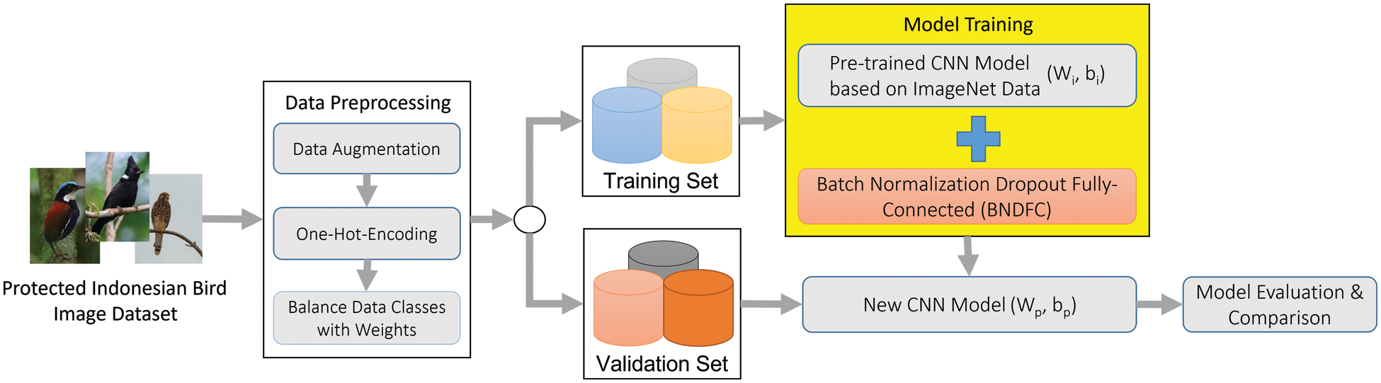
Figure 1: The workflow of the proposed approach
After data preparation, the model training is conducted using the pre-trained weights and bias of the baseline CNN model on ImageNet dataset. These pre-trained weights and biases are essentially used as initial parameters for the new model which will be used for training on another dataset, such as the PIB. Please note that this data preparation is the common step involved in any transfer learning application.
The proposed BNDFC layers with a specific sequence were suggested to be appended to the baseline model to improve the recognition performance. These layers include 1) BN layer which provides the normalized output with re-scaling and re-centering input values from the global average pooling layer, 2) D layer which randomly cancels out nodes in each iteration to prevent over-fitting, and 3) FC layer which combines the features detected from the figure patches with the data extracted by previous layers, and applies a linear transformation to the input vector through a weights matrix. The training of the baseline model with BNDFC was followed by the generation of a new set of weights and biases as (Wp, bp). The proposed BNDFC layers are explained comprehensively in Section 3.2.
3.1 Data Augmentation and Class Weights
Data augmentation has been addressed in [32] to resolve the issue of the limited size of the dataset. It was used to increase the number of images by manipulating original images without losing their essential features. The initial dataset used in this work consists of 8057 bird images which were further transformed as the training data [42] through rotation, horizontal and vertical shift, shear, zoom, and horizontal flip to increase the number of training images by following [34,43,44]. Moreover, the technique used for re-scaling in [45] was applied to the pixel range from [0,…, 255] to [0,…, 1]. The sample after data augmentation is presented in Fig. 2.
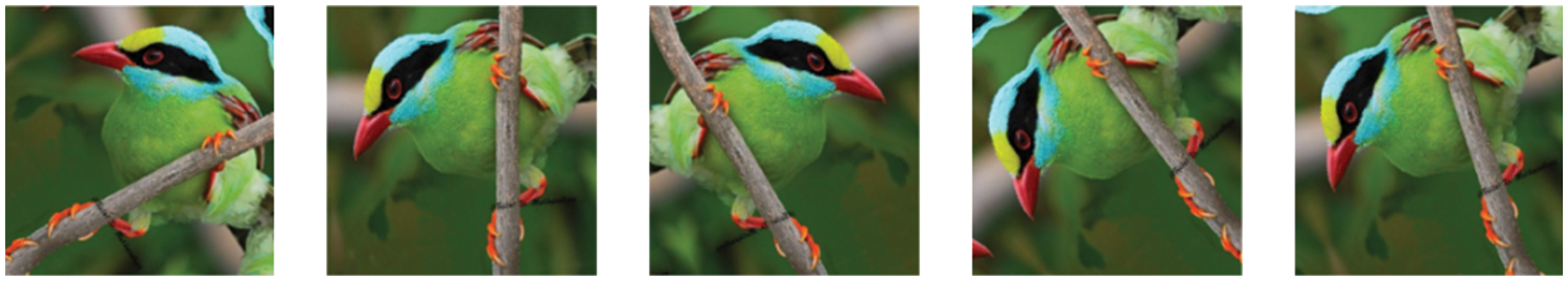
Figure 2: Sample augmentation technique–horizontal flip and rotation
The difficulty associated with obtaining PIB images led to the unevenness in the class of PIB collected. This unevenness might cause poor accuracy in the performance of those with a smaller number of images, as mentioned in [34]. Therefore, this research assigned different weight for each class by considering the number of image samples based on [46]. The formula used to calculate the weight of each class (Wi) is presented in the following Eq. (1). Essentially, for each class, the more number of images will lead to a smaller weight.
where
A Focal Loss (FL) was also applied in the training process to minimize the loss rate of training, while
where
3.2 Batch Normalization Dropout Fully-Connected (BNDFC) Layers
In this research, the proposed transfer learning is considered a weight initialization scheme as indicated by the baseline model which directly utilized the pre-trained weights and biases on the original ImageNet dataset as previously explained. The new dataset such as PIB in this present research was used to train the baseline model to update the weights and bias for obtaining the better accuracy. Meanwhile, the original baseline model was used as the features extractor by keeping its layers unchanged while the last layers before the output layer were replaced with the proposed sequence of BNDFC layers.
The details of the processes involved in appending the proposed sequence of BNDFC with the existing baseline model are illustrated in Fig. 3. As can be seen in Fig. 3, two networks were located from left to right. The first network is the baseline model for feature extraction. The standard input from each baseline model which matches the input trained on the ImageNet dataset was used in this research. It is important to note that a baseline model can be any CNN model trained based on ImageNet data. Fig. 3 illustrates the setting of MobileNetV2 which used the input of 224 × 224 × 3 vector [48] as an example.
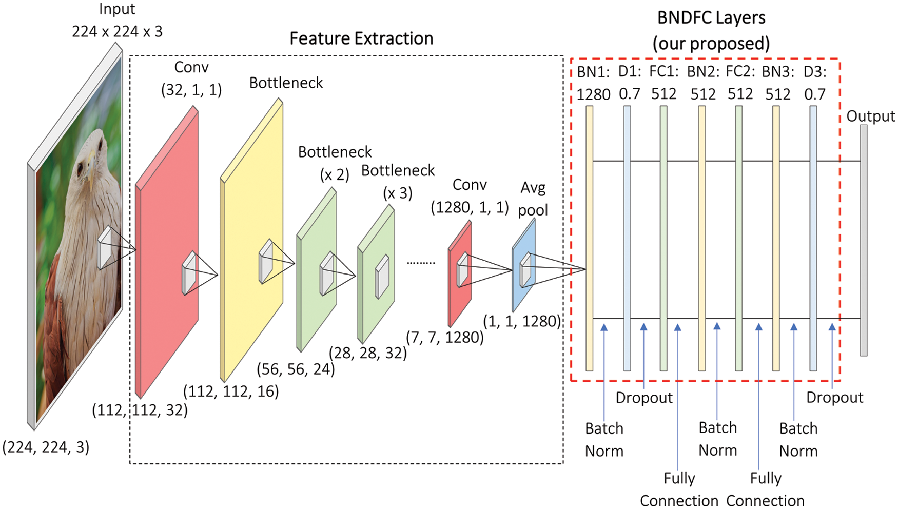
Figure 3: Illustration of the improve transfer learning based on baseline models using MobileNetV2 as an example
The second network on the right of Fig. 3 is the proposed sequence of BNDFC layers for weight and bias optimization. As commonly known, increasing the number of network layers seems to improve the accuracy [49]. However, focusing on improving the baseline model, the optimal size of the network is needed. Therefore, in this work, we further study how to combine the sequence of BN, D, and FC layers. The performance comparison of multiple sequence settings of BN, D, and FC layers was conducted and the results were shown in Section 4.2.
Based on the accuracy comparison, in this work, the optimal sequence of three BN, two FC layers, and two D were chosen to be placed between the feature extraction and the output layer. The first BN layer (BN1) was started at the end of the feature extraction layers of the baseline model to provide the normalized output by re-scaling and re-centering the input values. After BN1, the first D layer (D1) was placed to reduce over-fitting [50,51]. Two FC layers were applied to the input vector through the weight matrix. The objective of FC is to combine features detected from the image patches with the data extracted in previous layers after a linear transformation. The first FC layer (FC1) was applied to 512 neurons (dense) and placed after the first D layer (D1), while the second FC layer (FC2) was employed with 512 neurons (dense) and placed afterward. Moreover, the output of FC1 was normalized by placing the second BN layer (BN2) after FC1 and similarly the third BN layer (BN3) was placed after FC2. The second D layer (D2) was used to enhance the model and reduce the over-fitting again with the probability of retaining the unit at 0.7 before the output layer. Furthermore, one-dimensional output for the input image provided was generated in this model based on the number of classes to be predicted. The size was set at 83 in this research to be the same as the number of PIB species.
The FT technique was also used to re-train some of the layers of the baseline model by transferring their weights to the new model [33]. Several research works successfully used this method to improve the accuracy of models in several applications [30,33,34]. Moreover, the softmax used as an activation function represented in Eq. (3) was added to the FC layers.
where all the
As mentioned earlier, difference sequences of BNDFC were studied to investigate the optimal sequence of BNDFC layers. Then, the classification accuracy of baseline and baseline + BNDFC models were compared to evaluate the effectiveness of the proposed BNDFC layers. This experiment used 10 different pre-trained CNN models including DenseNet121 [52], Resnet50 [53], Resnet50V2 [54], VGG16, VGG19 [55], MobileNetV1 [56], MobileNetV2 [48], InceptionV3 [57], InceptionResnetV2 [58], and NasNetMobile [59] trained based on ImageNet dataset [37] as the baseline models. All of baseline models keep the original form of the pre-trained network using ImageNet (without appending BNDFC layers) which has 1000 categories. According to the dataset categories, the output layer on the baseline is the same as BNDFC, which is 83 neurons.
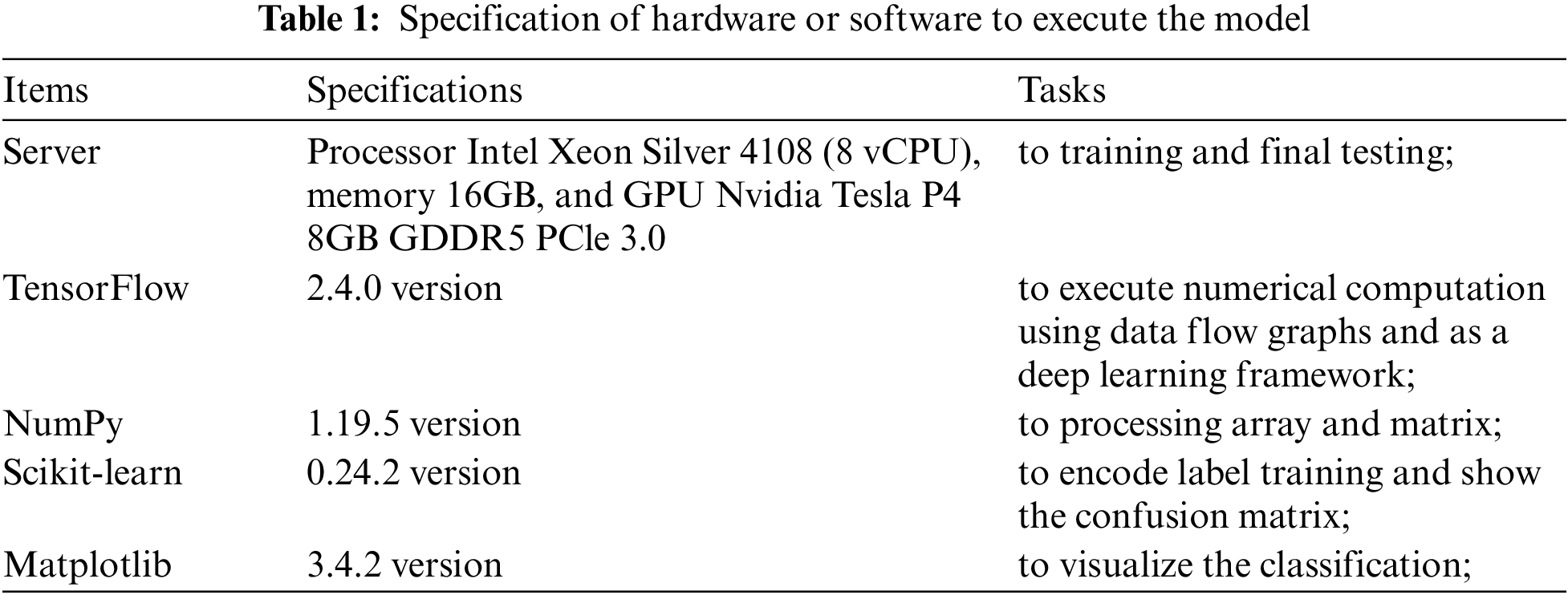
TensorFlow was used as a deep learning framework to support training on GPUs and build computation graphs descriptively for training and evaluation while Python wrapper library Keras was used as the back-end to design and construct the network models. The details of the environment, including the hardware, software, and library, are presented in Tab. 1.
The collection of an extensive dataset is a significant challenge in image classification [16] and is observed to be paramount in ensuring the success of the model. Therefore, 8057 figures of 83 categories of PIB were collected manually through photos or retrieved from the internet. These birds were captured by a Nikon Coolpix P1000 camera with 24-bit depth, 300 × 300 dpi resolution, and ISO-400 for ISO speed. The resolution of each figure was at least 224 × 224 pixels and a minimum of 46 figures were obtained from different views for each species. The dataset was later randomly divided into two sets based on [30,60–63]: a training set of 80% and a validation set of 20%. The samples used are indicated in the following Fig. 4.
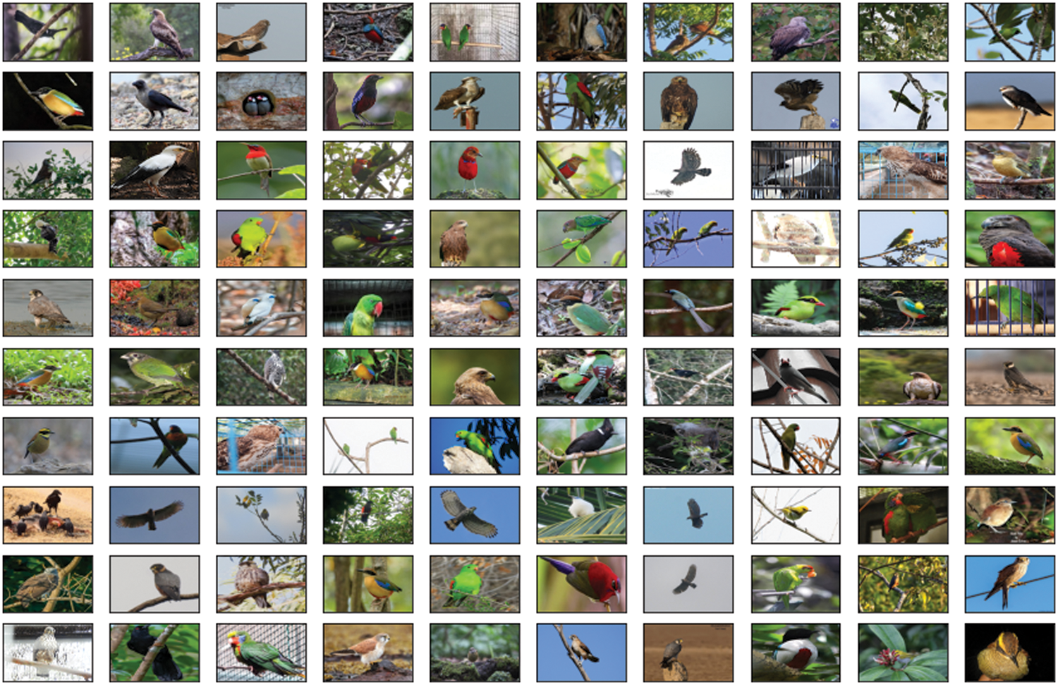
Figure 4: Samples of PIB images. (Sources: private property and Google images repository)
The experimental process was divided into three sections: the performance of the BNDFC model evaluation, the detailed evaluation of the training process, and a comparison of the model size. A detailed evaluation was also conducted on the training process of the baseline + BNDFC layers by combining two techniques which involved non-FT and FT. As previously explained, the FT technique was used to re-train the feature extraction layers of the baseline model by transferring its weights to the new model [33], while non-FT used the original weight of the baseline model without retraining their layers as indicated in [64]. The results of the detailed evaluation of the training process are also presented in Section 4.2.2. Moreover, the sizes of each model in terms of megabyte (MB) appended by the BNDFC layers were also evaluated and the results are indicated in Section 4.2.3.
Several environments, such as the ModelCheckpoint and the EarlyStopping functions in Tensorflow, were used for each training process. The ModelCheckpoint was used to define where to checkpoint the model weight, how the file should be named, and the circumstances to develop the model checkpoint. The EarlyStopping was used as the regularization tool to avoid over-fitting during the process of training a learner with an iterative method. They have both been applied in several research works mostly to maximize accuracy and minimize over-fitting [65,66].
The experimental performance of the baseline model and the baseline + BNDFC layers was evaluated using several metrics such as F-measure, G-mean, sensitivity, precision, fall-out, and miss rate with the results presented in Section 4.2.1. All of these functions are calculated based on elements of the confusion matrix: True-Positive (TP), False-Positive (FP), True-Negative (TN), and False-Negative (FN). The functions of the mentioned metrics are listed in Eqs. (4)–(9):
The F-measure was used to calculate the harmonic mean between precision and sensitivity.
G-mean or Geometric mean was calculated as the squared root of the product of the positive status against the correct classification and the negative status against the predicted negative status.
Sensitivity was utilized to calculate the proportion of the positive status against the correct classification.
Precision was utilized to calculate the positive patterns that are correctly predicted by all predicted patterns in a positive class.
Fall-out was used to determine the proportion of negative cases incorrectly identified as positive cases.
Miss rate was applied to calculate the ratio of FN to TP.
One of the main research works in this work is to study a special sequence of BNDFC which was proposed to improve accuracy. Tab. 2 compares the proposed sequence of BNDFC which has three BN, two FC layers, and two D with six other sequences of BN, D, and FC layers using MobileNetV2 as an example. Essentially, six sequences constructed by the combination of BN, D, and FC layers are compared with the proposed sequence of BNDFC. Three sequences have relatively shorter layers of the network representing the simpler networks, while another three sequences have relatively longer layers representing the complex network.
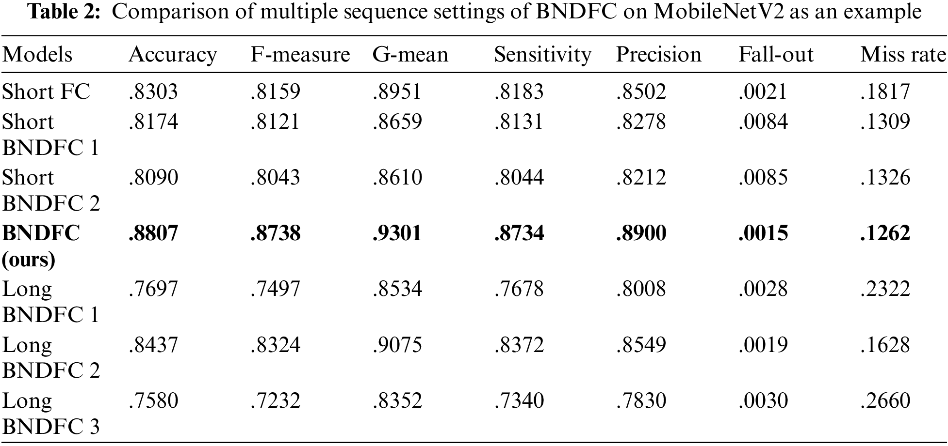
Short FC consists of only one FC layer to represent the simplest case. When combining BNDFC, two short versions were constructed. Short BNDFC 1 consists of one BN, D, and FC layer; and Short BNDFC 2 consists of two BN, one FC, and one D layers. For the long BNDFC, Long BNDFC 1 consists of four BN, three D, and three FC layers with sequence of BNDFC + BNFCBND + BNDFC; Long BNDFC 2 consists of five BN, three D, and three FC layers with sequence of BNDFC + BNFCBND + BNFCBND, and Long BNDFC 3 consists of six BN, four D, and four FC layers with sequence of BNDFC + BNFCBND + BNFCBND + BNDFC as the longest case.
As can be seen in Tab. 2, the result shows that the proposed sequence outperforms the network with other sequence settings on not only the accuracy but also all of the metric evaluations. Please also notice that the longer combination of BN, D, and FC cannot guarantee better performance on accuracy and other measures. This result proved that the specific BNDFC sequence proposed by this work has significant improvement. Therefore, in the following result, the proposed sequence of BNDFC was used for the comparison of baseline and baseline + BNDFC.
The performances of baseline with and without BNDFC were compared across 10 different network models. Tab. 3 shows the comparison results where the “Base” column presents the performance of the baseline model without BNDFC while “BNDFC” column shows the corresponding results after appending the BNDFC layers in the baseline (baseline + BNDFC). Except for fall-out and miss rate, the larger metric means the better performance.
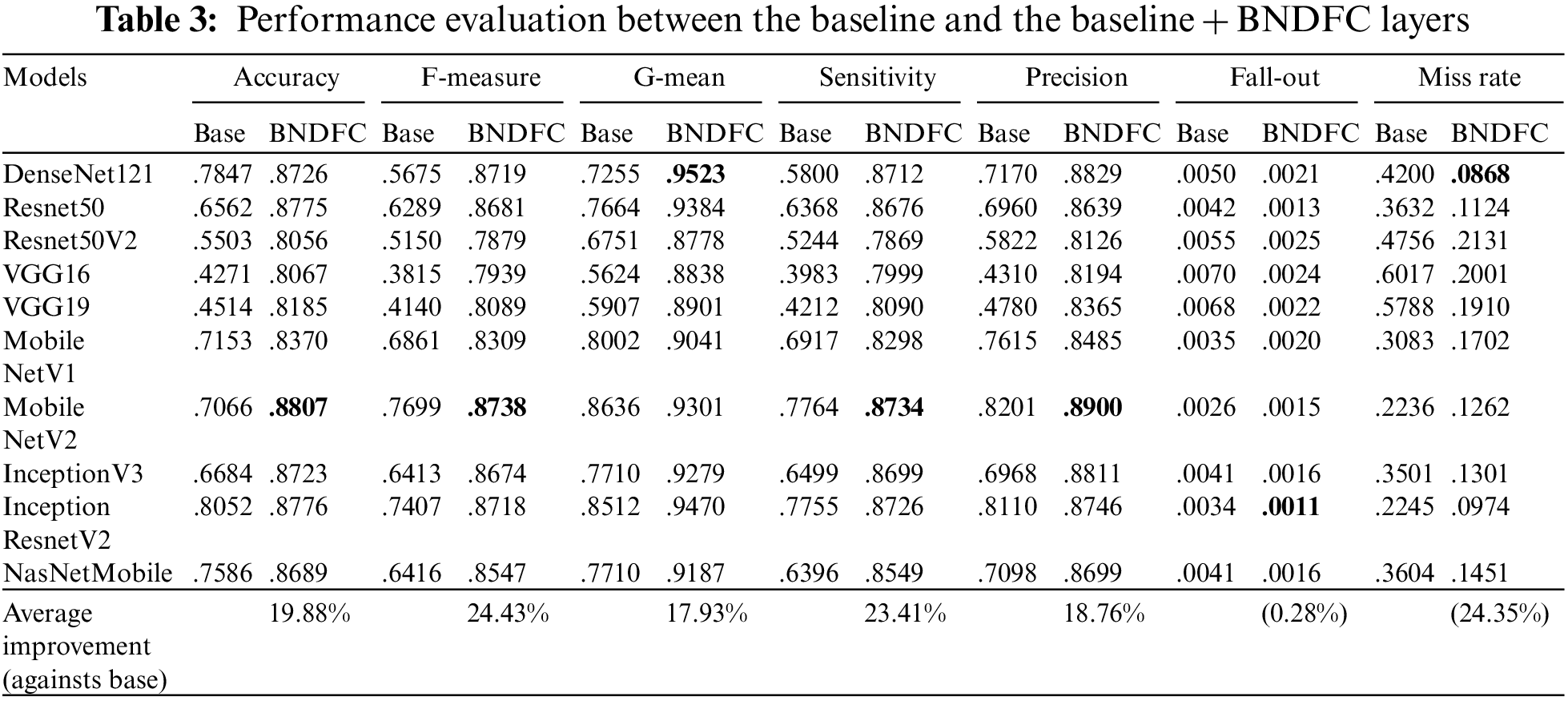
Obviously, all models with BNDFC have significant improvements against the baseline model in all of the above-mentioned metrics. As can be seen in the last row of Tab. 3, on average, appending the proposed BNDFC can improve 19.88% in Accuracy, 24.43% in F-measure, 17.93% in G-mean, 23.41% in Sensitivity, 18.76% in Precision. Also, adding BNDFC can improve by 0.28% in Fall-out and 24.35% in Miss rate (the lower is better), although the performance in Fall-out is not that significant.
For each metric, the bold-face number also indicates the model with the best performance model. Particularly, appending BNDFC layers in VGG16 can obtain the most improvement with 38.07% on average across 7 metrics, while InceptionResnetV2 has the less improvement with 9.2% across 7 metrics.
4.2.2 Training Process Evaluation
Tab. 4 shows the results of the training process on evaluating FT and non-FT under the models with BNDFC layers. The difference between FT and non-FT is in the training process. The non-FT case will train the model using the original weights of the feature extraction (baseline model), while the FT case will retrain all layers of the feature extraction (baseline model). Similarly, 10 models were evaluated based on metrics such as training accuracy, validation accuracy, training loss, and validation loss. Please note that the smaller training loss and validation loss are better.
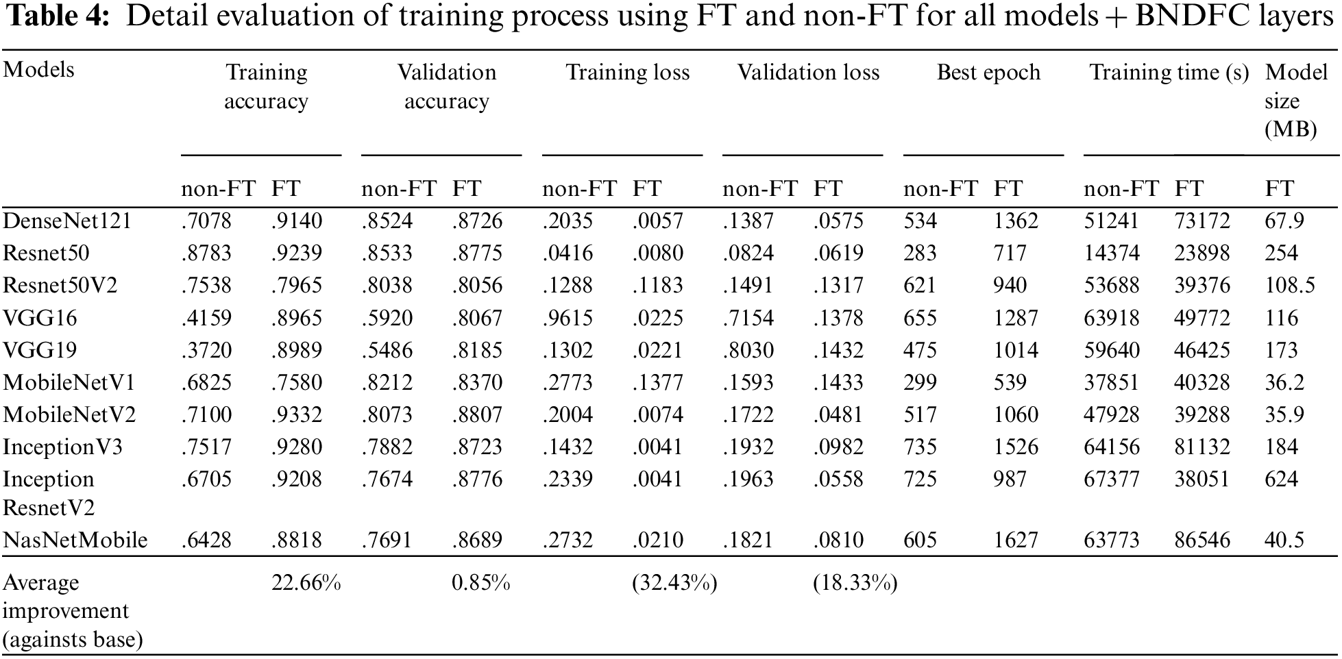
As can be seen in Tab. 4, applying FT can obtain higher training and validation accuracy with lower training and validation loss. On average across 10 models, the validation accuracy can be improved by 0.85% with a smaller validation loss by 18.33% improvement when comparing FT against non-FT. Tab. 4 also shows the number of epochs to reach the best result (Best Epoch), the number of epochs for stopping the training (Stop Epoch), and training time under FT and non-FT training. Without doubt, using FT will definitely consume more epoch (or time) for training, but the investment in training leads to a significant improvement in reducing the loss.
Fig. 5 visualizes the comparisons of accuracy and loss using MobileNetV2 as an example. In this case of MobileNetV2, the highest accuracy for the training and validation set are approximately 93.32% and 88.07%, respectively, after the FT was initiated in the epoch of 597 indicated by the green line after the accuracy and loss are stabilized during the original non-FT training process. After starting the FT process, the accuracy keeps going up while the loss is getting smaller. It also means the FT process can further improve the model without over-fitting (smaller loss). This result means the FT technique generally has the ability to improve the performance of the model either based on the accuracy or loss rate.
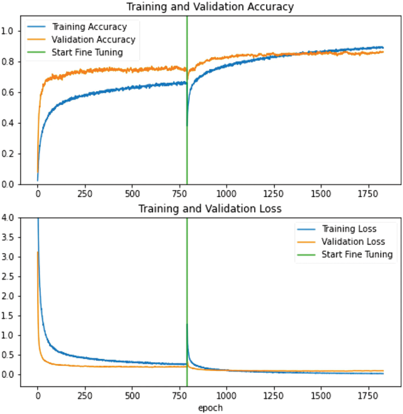
Figure 5: Visualization of accuracy and loss rate using FT and non-FT of on MobileNetV2 as an example
4.2.3 Comparison of Model Size
The size of model is another factor considered apart from the accuracy and loss rate. As addressed in [17,24,67], flexibility, computation ability, and capacity are important factors when applying deep learning networks on mobile platforms or portable devices [68]. Huge computation and millions of parameters are needed in large models [69], while mobile phones are constrained by memory size [17], and not recommended to use a large model with complex computation [68], the comparison regarding the size of model is also presented in the right column in Tab. 4. As can be seen, within models whose sizes are below 50 MB, MobileNetV2 is the only model which has more than 90% accuracy. The InceptionResnetV2, which had the second-highest accuracy, had a relatively large size that is almost 17.38 times that of MobileNetV2 in the validation set. In short, MobileNetV2 can be considered the cost-effective model based on the comparison.
This study proposed an improved transfer learning-based bird classification framework to achieve more accurate classification of PIB. The framework takes advantage of using the proposed sequence of BNDFC layers, which consist of BN, D, and FC layers to attach in the last layer of the traditional CNN model. Basically, the BN layer can provide the normalized output with re-scaling and re-centering input values from global average pooling. Also, the D layer randomly cancels nodes in each iteration to reduce the over-fitting. After the D layer, the FC layers are attached to combine the features detected from the figure patches extracted from the previous layers, and apply a linear transformation to the input vector through a weight matrix. Although the functions of BN, D, and FC have been studied in the literature, how to combine them as a sequence is not clear. This work tried to investigate the optimal sequence of combining BN, D, and FC as an attached layer after CNN-based model. Based on our study, a specific sequence of BNDFC was proposed to improve the performance on the accuracy and metric evaluations.
In this work, we not only extended the bird image database but also created the image variants for each collected PIB species. The database was used to evaluate the proposed BNDFC and FT methods. Based on the experimental results, accommodating BNDFC layers can achieve higher accuracy on both of training and validation datasets across ten different CNN-based models. On average, BNDFC can improve by 19.88% in Accuracy, 24.43% in F-measure, 17.93% in G-mean, 23.41% in Sensitivity, and 18.76% in Precision. In addition, applying FT can further improve the accuracy by 0.85% with a smaller validation loss by 18.33% improvement. MobileNetV2 was observed to be the best model with the lightest size of 35.9 MB and the highest accuracy of 88.07% in the validation set. The proposed sequence of BNDFC that can be applied to any CNN-based model to improve classification accuracy, is the main contribution of this study, particularly for image-based species classification challenges.
For the future work, it will be worthy to apply the proposed sequence of BNDFC on different deep learning models and evaluate the effectiveness. Also, it might be interesting to detect if the bird shown in the image is a live bird rather than a bird specimen. Last but not least, applying the proposed sequence of BNDFC layers to recognize other protected animals is another research direction.
Funding Statement: The authors appreciate the financial support from the Ministry of Science and Technology of Taiwan, (Contract No. 110-2221-E-011-140 and 109-2628-E-011-002-MY2) and the “Center for Cyber-Physical System Innovation” from The Featured Areas Research Center Program within the framework of the Higher Education Sprout Project by the Ministry of Education (MOE) in Taiwan. We also thank Pramana Yudha for Protection Indonesians Bird’s data sharing for this research work.
Conflicts of Interest: The authors declare that they have no conflicts of interest to report regarding the present study.
References
1. B. Indonesia, “Status burung di Indonesia 2021: Sembilan jenis burung semakin berisiko mengalami kepunahan,” 2021. [Online]. Available: http://www.burung.org/2021/04/28/. [Google Scholar]
2. F. S. Latumahina and G. Mardiatmoko, “Distribution of endemic birds in protected forests in Indonesia,” International Journal of Environmental and Science Education, vol. 14, no. 7, pp. 405–416, 2019. [Google Scholar]
3. M. Brambilla, F. Rizzolli, A. Franzoi, M. Caldonazzi, S. Zanghellini et al., “A network of small protected areas favoured generalist but not specialized wetland birds in a 30-year period,” Biological Conservation, vol. 248, pp. 108699, 2020. [Google Scholar]
4. K. Princé, P. Rouveyrol, V. Pellissier, J. Touroult and F. Jiguet, “Long-term effectiveness of natura 2000 network to protect biodiversity: A hint of optimism for common birds,” Biological Conservation, vol. 253, pp. 108871, 2021. [Google Scholar]
5. S. Chan, M. J. Crosby, M. Z. Islam, R. Rudyanto and A. W. Tordoff, “Important bird areas in Asia key sites for conservation,” in BirdLife Conservation Series, 13th ed., Cambridge, UK: BirdLife International, 2004. [Google Scholar]
6. R. M. Healey, J. R. Atutubo, M. D. Kusrini, L. Howard, F. Page et al., “Road mortality threatens endemic species in a national park in sulawesi, Indonesia,” Global Ecology and Conservation, vol. 24, pp. e01281, 2020. [Google Scholar]
7. A. S. Jati, H. Samejima, S. Fujiki, Y. Kurniawan, R. Aoyagi et al., “Effects of logging on wildlife communities in certified tropical rainforests in east kalimantan, Indonesia,” Forest Ecology and Management, vol. 427, no. 104, pp. 124–134, 2018. [Google Scholar]
8. M. Singh, “Evaluating the impact of future climate and forest cover change on the ability of southeast (SE) Asia’s protected areas to provide coverage to the habitats of threatened avian species,” Ecological Indicators, vol. 114, pp. 106307, 2020. [Google Scholar]
9. B. International, “Birdlife international (2021) country profile: Indonesia,” 2021. [Online]. Available: http://datazone.birdlife.org/country/indonesia. [Google Scholar]
10. C. R. Shepherd, B. T. C. Leupen, P. Siriwat and V. Nijman, “International wildlife trade, avian influenza, organised crime and the effectiveness of CITES: The Chinese hwamei as a case study,” Global Ecology and Conservation, vol. 23, pp. e01185, 2020. [Google Scholar]
11. K. M. Ragib, R. T. Shithi, S. A. Haq, M. Hasan, K. M. Sakib et al., “Pakhichini: Automatic bird species identification using deep learning,” in 2020 Fourth World Conf. on Smart Trends in Systems, Security and Sustainability (WorldS4), London, UK, pp. 1–6, 2020. [Google Scholar]
12. M. A. Tayal, “Bird identification by image recognition,” HELIX, vol. 8, no. 6, pp. 4349–4352, 2018. [Google Scholar]
13. S. Raj, S. Garyali, S. Kumar and S. Shidnal, “Image based bird species identification using convolutional neural network,” International Journal of Engineering Research and Technology, vol. 9, no. 6, pp. 346–351, 2020. [Google Scholar]
14. P. Gavali and J. S. Banu, “Bird species identification using deep learning on GPU platform,” in 2020 Int. Conf. on Emerging Trends in Information Technology and Engineering (ic-ETITE), Vellore, India, pp. 1–6, 2020. [Google Scholar]
15. J. Qin, W. Pan, X. Xiang, Y. Tan and G. Hou, “A biological image classification method based on improved CNN,” Ecological Informatics, vol. 58, pp. 101093, 2020. [Google Scholar]
16. A. C. Ferreira, L. R. Silva, F. Renna, H. B. Brandl, J. P. Renoult et al., “Deep learning-based methods for individual recognition in small birds,” Methods in Ecology and Evolution, vol. 11, no. 9, pp. 1072–1085, 2020. [Google Scholar]
17. Y. P. Huang and H. Basanta, “Bird image retrieval and recognition using a deep learning platform,” IEEE Access, vol. 7, pp. 66980–66989, 2019. [Google Scholar]
18. F. Mashuk, Samsujjoha, A. Sattar and N. Sultana, “Machine learning approach for bird detection,” in 2021 Third Int. Conf. on Intelligent Communication Technologies and Virtual Mobile Networks (ICICV), Tirunelveli, India, pp. 818–822, 2021. [Google Scholar]
19. J. Niemi and J. T. Tanttu, “Deep learning case study for automatic bird identification,” Applied Sciences, vol. 8, no. 11, pp. 1–15, 2018. [Google Scholar]
20. R. H. D. Zottesso, Y. M. G. Costa, D. Bertolini and L. E. S. Oliveira, “Bird species identification using spectrogram and dissimilarity approach,” Ecological Informatics, vol. 48, pp. 187–197, 2018. [Google Scholar]
21. R. Mohanty, B. Kumar Mallik and S. Singh Solanki, “Recognition of bird species based on spike model using bird dataset,” Data in Brief, vol. 29, pp. 105301, 2020. [Google Scholar]
22. P. Jancovic and M. Kokuer, “Bird species recognition using unsupervised modeling of individual vocalization elements,” IEEE/ACM Transactions on Audio Speech and Language Processing, vol. 27, no. 5, pp. 932–947, 2019. [Google Scholar]
23. Y. Harjoseputro, I. P. Yuda and K. P. Danukusumo, “MobileNets: Efficient convolutional neural network for identification of protected birds,” International Journal on Advanced Science, Engineering and Information Technology, vol. 10, no. 6, pp. 2290–2296, 2020. [Google Scholar]
24. K. Buschbacher, D. Ahrens, M. Espeland and V. Steinhage, “Image-based species identification of wild bees using convolutional neural networks,” Ecological Informatics, vol. 55, pp. 101017, 2020. [Google Scholar]
25. E. Meijering, “A Bird’s-eye view of deep learning in bioimage analysis,” Computational and Structural Biotechnology Journal, vol. 18, pp. 2312–2325, 2020. [Google Scholar]
26. Y. Harjoseputro, “A classification javanese letters model using a convolutional neural network with keras framework,” International Journal of Advanced Computer Science and Applications, vol. 11, no. 10, pp. 106–111, 2020. [Google Scholar]
27. A. Magotra and J. Kim, “Improvement of heterogeneous transfer learning efficiency by using hebbian learning principle,” Applied Sciences, vol. 10, no. 16, pp. 5631, 2020. [Google Scholar]
28. L. Alzubaidi, M. Al-Amidie, A. Al-Asadi, A. J. Humaidi, O. Al-Shamma et al., “Novel transfer learning approach for medical imaging with limited labeled data,” Cancers, vol. 13, no. 7, pp. 1590, 2021. [Google Scholar]
29. C. Iorga and V. -E. Neagoe, “A deep CNN approach with transfer learning for image recognition,” in 2019 11th Int. Conf. on Electronics, Computers and Artificial Intelligence (ECAI), Pitesti, Romani, pp. 1–6, 2019. [Google Scholar]
30. I. Dagher and D. Barbara, “Facial age estimation using pre-trained CNN and transfer learning,” Multimedia Tools and Applications, vol. 80, no. 13, pp. 20369–20380, 2021. [Google Scholar]
31. S. A. Hassan, M. S. Sayed, M. I. Abdalla and M. A. Rashwan, “Breast cancer masses classification using deep convolutional neural networks and transfer learning,” Multimedia Tools and Applications, vol. 79, no. 41, pp. 30735–30768, 2020. [Google Scholar]
32. D. Zhang, J. Hu, F. Li, X. Ding, A. K. Sangaiah et al., “Small object detection via precise region-based fully convolutional networks,” Computers, Materials and Continua, vol. 69, no. 2, pp. 1503–1517, 2021. [Google Scholar]
33. E. Baykal, H. Dogan, M. E. Ercin, S. Ersoz and M. Ekinci, “Transfer learning with pre-trained deep convolutional neural networks for serous cell classification,” Multimedia Tools and Applications, vol. 79, no. 21, pp. 15593–15611, 2020. [Google Scholar]
34. S. Chakraborty, R. Mondal, P. K. Singh, R. Sarkar and D. Bhattacharjee, “Transfer learning with fine tuning for human action recognition from still images,” Multimedia Tools and Applications, vol. 80, no. 13, pp. 20547–20578, 2021. [Google Scholar]
35. M. Mathur, D. Vasudev, S. Sahoo, D. Jain and N. Goel, “Crosspooled FishNet: Transfer learning based fish species classification model,” Multimedia Tools and Applications, vol. 79, no. 41, pp. 31625–31643, 2020. [Google Scholar]
36. X. Zhang, J. Zhou, W. Sun and S. K. Jha, “A lightweight CNN based on transfer learning for COVID-19 diagnosis,” Computers, Materials and Continua, vol. 72, no. 1, pp. 1123–1137, 2022. [Google Scholar]
37. D. Jia, D. Wei, R. Socher, L. Li-Jia, L. Kai et al., “ImageNet: A large-scale hierarchical image database,” in 2009 IEEE Conf. on Computer Vision and Pattern Recognition, Miami, FL, USA, pp. 248–255, 2009. [Google Scholar]
38. M. Z. Ur Rehman, F. Ahmed, M. A. Khan, U. Tariq, S. S. Jamal et al., “Classification of citrus plant diseases using deep transfer learning,” Computers, Materials and Continua, vol. 70, no. 1, pp. 1401–1417, 2021. [Google Scholar]
39. U. -O. Dorj, K. -K. Lee, J. -Y. Choi and M. Lee, “The skin cancer classification using deep convolutional neural network,” Multimedia Tools and Applications, vol. 77, no. 8, pp. 9909–9924, 2018. [Google Scholar]
40. A. Taner, Y. B. Öztekin and H. Duran, “Performance analysis of deep learning CNN models for variety classification in hazelnut,” Sustainability, vol. 13, no. 12, pp. 6527, 2021. [Google Scholar]
41. N. Sarafianos, X. Xu and I. A. Kakadiaris, “Deep imbalanced attribute classification using visual attention aggregation,” in European Conf. on Computer Vision (ECCV), Munich, Germany, pp. 708–725, 2018. [Google Scholar]
42. S. Zhou, M. Ke and P. Luo, “Multi-camera transfer GAN for person re-identification,” Journal of Visual Communication and Image Representation, vol. 59, pp. 393–400, 2019. [Google Scholar]
43. W. Wei, J. Yongbin, L. Yanhong, L. Ji, W. Xin et al., “An advanced deep residual dense network (DRDN) approach for image super-resolution,” International Journal of Computational Intelligence Systems, vol. 12, no. 2, pp. 1592–1601, 2019. [Google Scholar]
44. W. Wang, Y. Yang, J. Li, Y. Hu, Y. Luo et al., “Woodland labeling in Chenzhou, China, via deep learning approach,” International Journal of Computational Intelligence Systems, vol. 13, no. 1, pp. 1393–1403, 2020. [Google Scholar]
45. P. Paul, M. A. -U. -A. Bhuiya, M. A. Ullah, M. N. Saqib, N. Mohammed et al., “A modern approach for sign language interpretation using convolutional neural network,” in PRICAI 2019: Trends in Artificial Intelligence, Cuvu, Yanuca Island, Fiji, pp. 431–444, 2019. [Google Scholar]
46. Z. Hu, B. Tan, R. Salakhutdinov, T. Mitchell and E. P. Xing, “Learning data manipulation for augmentation and weighting,” in 33rd Conf. on Neural Information Processing Systems, Vancouver, Canada, pp. 15764–15775, 2019. [Google Scholar]
47. T. Y. Lin, P. Goyal, R. Girshick, K. He and P. Dollar, “Focal loss for dense object detection,” IEEE Transactions on Pattern Analysis and Machine Intelligence, vol. 42, no. 2, pp. 318–327, 2020. [Google Scholar]
48. M. Sandler, A. Howard, M. Zhu, A. Zhmoginov and L. C. Chen, “MobileNetv2: Inverted residuals and linear bottlenecks,” in IEEE Conf. on Computer Vision and Pattern Recognition (CVPR), Salt Lake, Utah, United States, pp. 4510–4520, 2018. [Google Scholar]
49. M. Uzair and N. Jamil, “Effects of hidden layers on the efficiency of neural networks,” in 2020 IEEE 23rd Int. Multitopic Conf. (INMIC), Bahawalpu, Pakistan, pp. 1–6, 2020. [Google Scholar]
50. S. Park and N. Kwak, “Analysis on the dropout effect in convolutional neural networks,” in 13th Asian Conf. on Computer Vision, Taipei, Taiwan, pp. 189–204, 2016. [Google Scholar]
51. N. Srivastava, G. Hinton, A. Krizhevsky, I. Sutskever and R. Salakhutdinov, “Dropout: A simple way to prevent neural networks from overfitting,” Journal of Machine Learning Research, vol. 15, no. 1, pp. 1929–1958, 2014. [Google Scholar]
52. G. Huang, Z. Liu, L. Van Der Maaten and K. Q. Weinberger, “Densely connected convolutional networks,” in 2017 IEEE Conf. on Computer Vision and Pattern Recognition (CVPR), Honolulu, USA, pp. 2261–2269, 2017. [Google Scholar]
53. K. He, X. Zhang, S. Ren and J. Sun, “Deep residual learning for image recognition,” in 2016 IEEE Conf. on Computer Vision and Pattern Recognition (CVPR), Las Vegas, USA, pp. 770–778, 2016. [Google Scholar]
54. K. He, X. Zhang, S. Ren and J. Sun, “Identity mappings in deep residual networks,” in 14th European Conf. on Computer Vision, Amsterdam, Netherlands, pp. 630–645, 2016. [Google Scholar]
55. K. Simonyan and A. Zisserman, “Very deep convolutional networks for large-scale image recognition,” arXiv preprint arXiv:1409.1556, pp. 1–9, 2014. [Google Scholar]
56. A. G. Howard, M. Zhu, B. Chen, D. Kalenichenko, W. Wang et al., “MobileNets: Efficient convolutional neural networks for mobile vision applications,” arXiv preprint arXiv:1704.04861, pp. 1–9, 2017. [Google Scholar]
57. C. Szegedy, V. Vanhoucke, S. Ioffe, J. Shlens and Z. Wojna, “Rethinking the inception architecture for computer vision,” in 2016 IEEE Conf. on Computer Vision and Pattern Recognition (CVPR), Las Vegas, USA, pp. 2818–2826, 2016. [Google Scholar]
58. C. Szegedy, S. Ioffe, V. Vanhoucke and A. Alemi, “Inception-v4, inception-ResNet and the impact of residual connections on learning,” in AAAI’17: Proc. of the Thirty-First AAAI Conf. on Artificial Intelligence, San Francisco, California, USA, pp. 4278–4284, 2017. [Google Scholar]
59. B. Zoph, V. Vasudevan, J. Shlens and Q. V. Le, “Learning transferable architectures for scalable image recognition,” in IEEE Conf. on Computer Vision and Pattern Recognition (CVPR), Salt Lake, Utah, United States, pp. 8697–8710, 2018. [Google Scholar]
60. M. E. Karar, O. Reyad, M. Abd-Elnaby, A. H. Abdel-Aty and M. A. Shouman, “Lightweight transfer learning models for ultrasound-guided classification of COVID-19 patients,” Computers, Materials and Continua, vol. 69, no. 2, pp. 2295–2312, 2021. [Google Scholar]
61. S. Afzal, I. U. Khan and J. W. Lee, “A transfer learning-based approach to detect cerebral microbleeds,” Computers, Materials and Continua, vol. 71, no. 1, pp. 1903–1923, 2022. [Google Scholar]
62. T. M. Ghazal, S. Abbas, S. Munir, M. A. Khan, M. Ahmad et al., “Alzheimer disease detection empowered with transfer learning,” Computers, Materials and Continua, vol. 70, no. 3, pp. 5005–5019, 2022. [Google Scholar]
63. W. Wang, H. Liu, J. Li, H. Nie and X. Wang, “Using CFW-net deep learning models for X-ray images to detect COVID-19 patients,” International Journal of Computational Intelligence Systems, vol. 14, no. 1, pp. 199–207, 2021. [Google Scholar]
64. H. Cao, S. Bernard, L. Heutte and R. Sabourin, “Improve the performance of transfer learning without fine-tuning using dissimilarity-based multi-view learning for breast cancer histology images,” in 15th Int. Conf. on Image Analysis and Recognition, Póvoa de Varzim, Portugal, pp. 779–787, 2018. [Google Scholar]
65. J. Barry-Straume, A. Tschannen, D. W. Engels and E. Fine, “An evaluation of training size impact on validation accuracy for optimized convolutional neural networks,” SMU Data Science Review, vol. 1, no. 4, pp. 12–29, 2018. [Google Scholar]
66. H. Lee and J. Song, “Introduction to convolutional neural network using keras; An understanding from a statistician,” Communications for Statistical Applications and Methods, vol. 26, no. 6, pp. 591–610, 2019. [Google Scholar]
67. Y. Harjoseputro, Y. D. Handarkho and H. T. R. Adie, “The javanese letters classifier with mobile client-server architecture and convolution neural network method,” International Journal of Interactive Mobile Technologies, vol. 13, no. 12, pp. 67–80, 2019. [Google Scholar]
68. J. Wang, Y. Wu, S. He, P. K. Sharma, X. Yu et al., “Lightweight single image super-resolution convolution neural network in portable device,” KSII Transactions on Internet and Information Systems, vol. 15, no. 11, pp. 4065–4083, 2021. [Google Scholar]
69. S. He, Z. Li, Y. Tang, Z. Liao, F. Li et al., “Parameters compressing in deep learning,” Computers, Materials and Continua, vol. 62, no. 1, pp. 321–336, 2020. [Google Scholar]
 | This work is licensed under a Creative Commons Attribution 4.0 International License, which permits unrestricted use, distribution, and reproduction in any medium, provided the original work is properly cited. |