Computers, Materials & Continua DOI:10.32604/cmc.2022.031324
Article

Biomedical Osteosarcoma Image Classification Using Elephant Herd Optimization and Deep Learning

Areej A. Malibari1, Jaber S. Alzahrani2, Marwa Obayya3, Noha Negm4,5, Mohammed Abdullah Al-Hagery6, Ahmed S. Salama7 and Anwer Mustafa Hilal8,*

1Department of Industrial and Systems Engineering, College of Engineering, Princess Nourah Bint Abdulrahman University, P.O. Box 84428, Riyadh, 11671, Saudi Arabia
2Department of Industrial Engineering, College of Engineering at Alqunfudah, Umm Al-Qura University, Saudi Arabia
3Department of Biomedical Engineering, College of Engineering, Princess Nourah Bint Abdulrahman University, P.O. Box 84428, Riyadh, 11671, Saudi Arabia
4Department of Computer Science, College of Science & Art at Mahayil, King Khalid University, Saudi Arabia
5Faculty of Science, Mathematics and Computer Science Department, Menoufia University, Egypt
6Department of Computer Science, College of Computer, Qassim University, Saudi Arabia
7Department of Electrical Engineering, Faculty of Engineering & Technology, Future University in Egypt, New Cairo, 11845, Egypt
8Department of Computer and Self Development, Preparatory Year Deanship, Prince Sattam Bin Abdulaziz University, AlKharj, Saudi Arabia
*Corresponding Author: Anwer Mustafa Hilal. Email: a.hilal@psau.edu.sa
Received: 14 April 2022; Accepted: 07 June 2022

Abstract: Osteosarcoma is a type of malignant bone tumor that is reported across the globe. Recent advancements in Machine Learning (ML) and Deep Learning (DL) models enable the detection and classification of malignancies in biomedical images. In this regard, the current study introduces a new Biomedical Osteosarcoma Image Classification using Elephant Herd Optimization and Deep Transfer Learning (BOIC-EHODTL) model. The presented BOIC-EHODTL model examines the biomedical images to diagnose distinct kinds of osteosarcoma. At the initial stage, Gabor Filter (GF) is applied as a pre-processing technique to get rid of the noise from images. In addition, Adam optimizer with MixNet model is also employed as a feature extraction technique to generate feature vectors. Then, EHO algorithm is utilized along with Adaptive Neuro-Fuzzy Classifier (ANFC) model for recognition and categorization of osteosarcoma. EHO algorithm is utilized to fine-tune the parameters involved in ANFC model which in turn helps in accomplishing improved classification results. The design of EHO with ANFC model for classification of osteosarcoma is the novelty of current study. In order to demonstrate the improved performance of BOIC-EHODTL model, a comprehensive comparison was conducted between the proposed and existing models upon benchmark dataset and the results confirmed the better performance of BOIC-EHODTL model over recent methodologies.

Keywords: Biomedical imaging; osteosarcoma classification; deep transfer learning parameter tuning; fuzzy logic

1  Introduction

Osteosarcoma is a type of primary bone malignancy reported among children, teens and young adults, according to American cancer society. The present treatment modality comprises of surgery and neoadjuvant chemotherapy which have significantly increased the five-years’ survival rate of osteosarcoma-affected patients. Between 1975 and 2010, there was an increase found in five-years’ survival rate from 40 to 76 percent among osteosarcoma children aged below 15 years and from 56 to 66 percent among adolescent elders aged between 15 and 19 years [1]. But the prognosis for patient who develops distal metastases is still miserable. The five-years’ survival rate for metastatic Osteosarcoma is less than 20 percent. In medical settings, metastasectomy is one of the approaches to cure metastatic osteosarcoma that demands early diagnosis of metastasis. However, it is challenging to diagnose the early stages of disease development, due to sub-medical manifestation. Moreover, high rate of pulmonary metastases, increasing frequency of chemo-resistance, and non-targeted therapy are some of the challenges involved in treatment process. Osteosarcoma harbor highly complicated genomic landscape, and heterogeneity within as well as among tumors [2]. Until now, no target mutation is authenticated to increase the treatment of this lethal disease [3].

Primary bone tumors are accountable for 5–10 percent of each pediatric tumor diagnosed every year. Osteosarcoma is a primary form of malignant primary bone cancer. Notwithstanding the restricted 1,000 new cases every year in the United States, the prognoses of osteosarcoma remain a challenge [4]. Two age peaks of occurrence are observed such as people at adolescent stage i.e., age range of 10–20 and the peak age of children under 10 years. Usually, Osteosarcoma starts at the metaphysis of long bones in low limbs which is accountable for 40–50 percent of overall cases [5]. Usually, osteosarcoma symptoms include redness, warmth at the site of tumor, and mild localized bone pain. The patient experiences an increase in pain in the course of time and it frequently affects the patient’s movement and joint functions. If osteosarcoma is not diagnosed at early stages, it is predicted to reach a wide-range of metastasis that include lungs, soft tissues, and other bones [6]. Magnetic Resonance Images (MRI), histological biopsy tests, and X-rays are important diagnostic methods that are currently under use for osteosarcoma diagnosis. At present, the diagnosis of osteosarcoma comprises of physical examinations and a comprehensive patient history analysis [7].

Typically, the presented symptoms include constant, deep-seated, swelling, and gnawing pain at the stimulated site. Pain in various regions might portend skeletal metastasis; thus, it needs to be properly examined [8]. With regards to disease diagnosis, the normal investigation methods for the assessment of possible osteosarcoma include laboratory tests, X-ray of the infected bone, chest Computed Tomography (CT) scan, Magnetic Resonance Imaging (MRI) scans of the infected bone, whole-body technetium bone scan, percutaneous image-guided biopsy and chest X-ray [9]. Even though biopsy-based method identifies the malignancy in an efficient manner, the limitation of histological-guided biopsies and MRI scans has constrained the detection ability. In addition, histological specimen-based investigation is a laborious process. For instance, a precise diagnosis of osteosarcoma malignancy needs the investigation of a minimum of 50 histology slides to denote a plane of large 3D tumors [10]. In this background, the current study proposes the application of Artificial Intelligence and Machine Learning models for early diagnosis of osteosarcoma. Fig. 1 illustrates the contributions of AI in healthcare system.

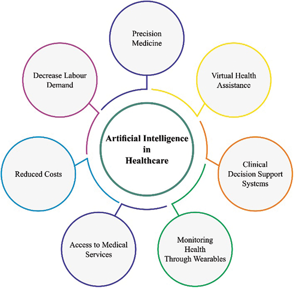
Figure 1: AI in healthcare

In literature [11], Deep Learning (DL) and Machine Learning (ML) fusion models have been validated for classification of malignant, benign, and intermediate bone tumors based on patient’s clinical features and traditional radiographs of the lesion. DL and ML fusion methods have also been developed for classification of tumors by traditional radiographs of the lesion and potentially appropriate clinical data. In the study conducted earlier [12], a DL-related osteosarcoma classification algorithm was suggested using ensemble approach and fusion approach. Multilevel features can be derived from a pre-trained Efficient Nets which is well trained on imagenet1k dataset. Efficient Nets are embedded with Convolutional Neural Networks (CNN) in terms of resolution, width, and depth. The features are derived from opening layers, intermediate layers, and the last layers of the chosen Efficient Net. The features are provided to fault-control output coding classifiers autonomously with Support Vector Machine as base learner.

The authors [13] presented an efficient detection technique to diagnose osteosarcoma at early stages and the technique is enhanced by the suggested Fractional-Harris Hawks Optimization-related Generative Adversarial Network (F-HHO-based GAN). Here, the suggested F-HHO was created by integrating HHO, Fractional and Calculus correspondingly. Tumor categorization was performed by GAN with the help of histological image slides. Bansal et al. [14–17] exhibited the advancements and implemented a Computer-Aided Diagnosis (CAD) system on the basis of image processing, deep learning, and machine learning techniques. The datasets used were composed of Hematoxylin and Eosin (H&E)-stained histology images, received by biopsy centers, at distinct phases of cancer. The features were derived after image segmentation process. CNN is designed or customized for categorization of tumors amongst patients into four categories.

The current study introduces a new Biomedical Osteosarcoma Image Classification using Elephant Herd Optimization and Deep Transfer Learning (BOIC-EHODTL) model. The presented BOIC-EHODTL model examines the biomedical images for the occurrence of distinct kinds of osteosarcoma. At the initial stage, Gabor Filter (GF) is applied as a pre-processing technique to get rid of the noise from images. In addition, Adam optimizer with MixNet model is also employed as a feature extraction technique to generate feature vectors. Followed by, EHO algorithm with Adaptive Neuro-Fuzzy Classifier (ANFC) model is utilized for recognition and categorization of osteosarcoma. In order to demonstrate the improved performance of BOIC-EHODTL model, a comprehensive comparison study was conducted on benchmark dataset.

2  The Proposed Model

In this study, a novel BOIC-EHODTL model has been developed for the investigation of biomedical images to identify distinct kinds of osteosarcoma. Primarily, GF technique is employed as a pre-processing technique to get rid of the noise from images. At the same time, Adam optimizer with MixNet model is also employed as a feature extraction technique to generate feature vectors. Moreover, EHO algorithm, with ANFC model, is also utilized for recognition and categorization of osteosarcoma. Fig. 2 illustrates the block diagram of BOIC-EHODTL technique.

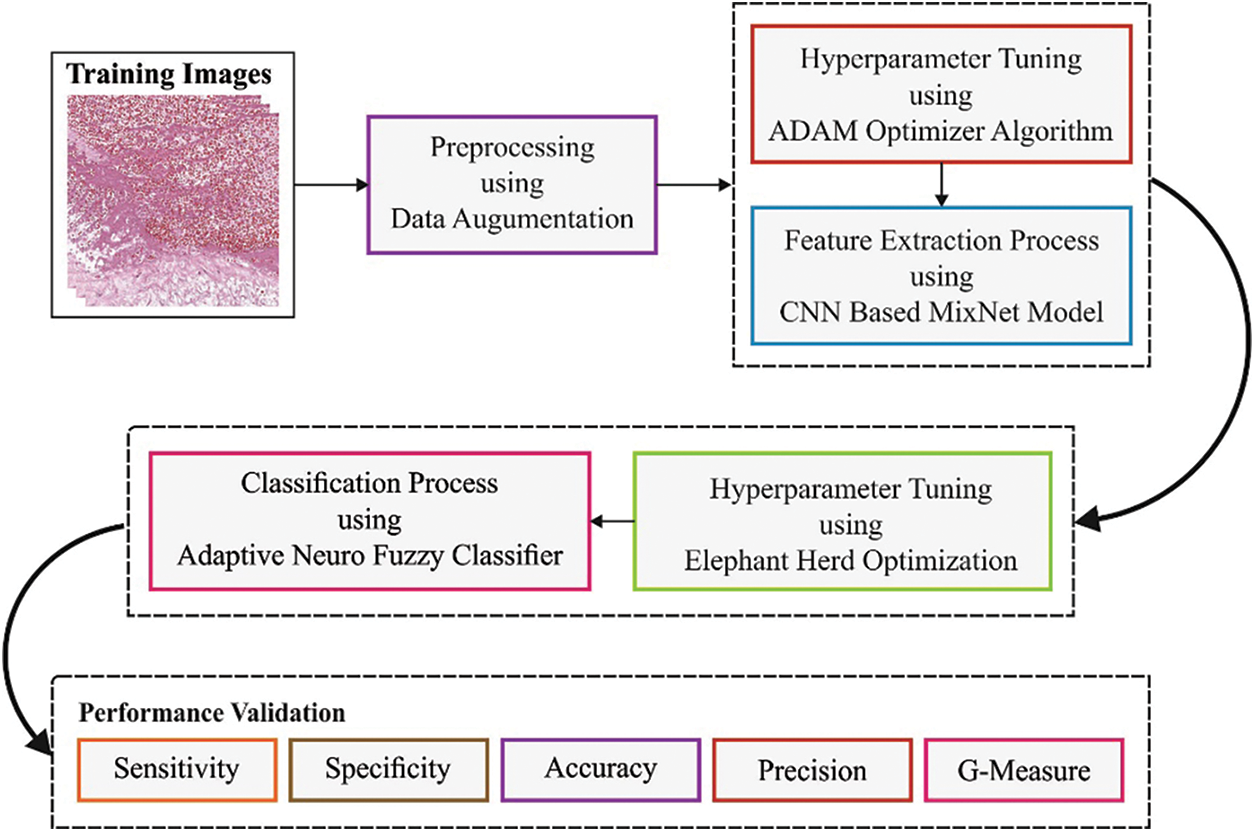
Figure 2: Block diagram of BOIC-EHODTL technique

2.1 Image Pre-Processing

At the initial stage, GF technique is employed as a pre-processing technique to get rid of the noise. GF is a bandpass filter that is widely used to remove noise. In 2-D coordinate (a,b) system, GF comprises of real and imaginary components as given below.

Gδ,θ,ψ,σ,γ(a,b)=exp⁡(−a′2+γ2b′22σ2)×exp⁡(j(2πa′δ+ψ))(1)

where

a′=acos⁡θ+bsin⁡θ(2)

b′=−asin⁡θ+bcos⁡θ(3)

where δ denotes the sinusoidal factor wavelength, and θ denotes the orientation separation angle of Gabor kernels.

2.2 Feature Extraction

After image pre-processing, Adam optimizer with MixNet model is employed as a feature extraction technique to generate feature vectors [18]. In general, it is an observation that good efficiency and accuracy are attained by imposing a balance among each dimension of the network. So, EfficientNet is presented to improve the efficiency of Convolution Neural Network (CNN) by scaling in 3D values i.e., resolution, width, and depth, with a subset of scaling coefficients that meet certain constraints. With a total of 18 convolutional layers i.e., D = 18, all the layers are armed with kernel k(3,3) or k(5,5). The input image contains R, G, and B channels that correspond to the size, 224 × 224. The second layer is scaled down in terms of resolution to minimize the feature map size, while on the other hand, it is scaled up in terms of width to improve the performance. For example, the next convolution layer contains W = 16 filters, and the amount of filters using second convolutional layer is W = 24. The maximal amount of filters is D = 1,280 and for the final layer, it is 200 which is fed to Fully Connected (FC) layer. It uses k(3,3), k(5,5), or k(7,7) kernels. But large kernel tends to enhance both efficiency and accuracy. Moreover, large kernel assists in capturing high-resolution patterns, whereas smaller kernels allows the extraction of low-resolution patterns. In order to retain a balance between efficiency and accuracy, MixNet family is constructed on the basis of MobileNet architecture. It has an aim to achieve i.e., to reduce FLOPs and the number of parameters.

Adam optimization, ‘Adaptive Moment estimate optimization’ follows an approach for 1st-order gradient-based optimization [19]. It depends upon adaptive estimate of low-order moment. At this point, gt signifies the gradient, θt represents the parameter at time t, β1 and β2 go to [0,1], and α signifies the rate of learning. gt2 represents element-wise square of gt⊙gt and projects the default settings i.e., α = 0.001, β1 = 0.9, β2 = 0.999, and ε=10−8. All the procedures on vector are determined element-wise, while β1t and β2t represent β1 and β2 to the power of t.

2.3 Image Classification

For image classification, ANFC model is utilized to recognize and categorize osteosarcoma [20]. ANFC structural method is a dynamic network that utilizes supervised learning method and is similar to Takagi-Sugeno method. Assume a set of two inputs, x and y between which one output f has the structure. A collection of if-then rules is employed and sample rules are shown herewith.

•   Rule 1: If x is A1 and y is B1 Then f1=p1x+q1y+r1.

•   Rule 2: If x is A2 and y is B2 Then f2=p2x+q2y+r2.

Here A1,A2 and B1,B2 indicate the membership functions of input x and y, p1,q1,r1 and p2,q2,r2 indicate the linear variables that exist in the resulting portion of Takagi-Sugeno method. ANFC structure involves five layers as demonstrated in the following section. The 1st and 4th layers include an adoptive node, while the residual layer has a static node.

Layer 1

All the nodes might adapt themselves to a function variable. The outcome, from all the nodes, is a degree of membership value that is represented by the input of membership function. Especially, bell-shaped Membership Function (MF) is applied as given below.

μAi(x)=11+|x−ca|2b(4)

Here, μAi indicates the degree of MF for fuzzy set Ai, and {a,b,c} denotes the variable of MF which alters its shape.

Layer 2

All the nodes in the layer are either static or pre-determined with a product operator, Π. It describes the firing strength of all the rules.

Layer 3

All the nodes in this layer are static or non-adoptive and are represented as N. It standardizes the firing strength i.e., w¯i=wi/Σwi.

Layer 4

All the nodes in this layer are dynamic in nature with a function as given below.

w¯ifi=pix+qiy+ri(5)

The variable in this layer is determined by the succeeding parameters.

Layer 5

All the nodes in this layer are either static or non-dynamic that define the overall results by calculating the received signals from previous node as Σw¯ifi.

Both 1st and 4th layers involve the adjustable variables in training phase. Epoch rate, MF, and fuzzy rule amount should be accurately selected using ANFC proposal after which the result is achieved for data over-fitting. It can be performed by integrating the least-square with gradient descent method.

2.4 Parameter Optimization

In this final stage, EHO algorithm is applied to fine tune the parameters [21–24] involved in ANFC model [25]. EHO technique is performed with the help of characterized procedures, while the performance is determined as given herewith; Assume an elephant clan to be ci. Next, the upcoming location of elephant is j in a clan and is upgraded by the following equation.

xnew,ci,j=xci,j+α×(xbest,ci−xci,j)×r,(6)

whereas xnew,ci,j demonstrates the extended position, xci,j represents the latest place of an elephant j in clan ci. xbest,ci indicates a matriarch of clan ci; in which female is an optimum elephant. A scaling factor α∈[0,1] defines the efficacy of leader i.e., ci on xci,j. r∈[0,1], while it is determined as a stochastic distribution that offers a better objective in diversified population. Recently, a standard distribution is exploited. It is apparent that xci,j=xbest,ci, indicates that a matriarch in a clan could not be upgraded. So, it is removed by expanding the optimum elephant using the following equation.

xnew,ci,j=β×xcenter,ci,(7)

Here, the power of xcenter,ci on xnew,ci, is normalized using β∈[0,1]. The dataset from an individual in clan ci is utilized for the development of a novel individual xnew,ci,j. The intermediate of clan ci, xcenter,ci, can be evaluated for d-th dimension vector using D calculation, where D denotes the whole dimension as follows:

xcenter,ci,d=1nci×∑j=1ncixci,j,d(8)

Now, 1≤d≤D denotes d-th dimensional vector, nci indicates the count of individuals in ci, xci,j,d indicates the d th dimensional vector of individual xci,j. In each clan, male elephant leaves the family and lives individually, when it grows as an adult. This separation is called isolation operator, thus the optimization problem is resolved. In order to enhance the exploration capability of EHO technique, consider that an elephant with poor fitness can execute a separate operator for all the generations as given below.

xworst,ci=xmin+(xmax−xmin+1)×rand(9)

Now xmax and xmin indicate the upper and lower limits, correspondingly. xworst,ci describes the lesser individual elephant in clan ci. rand∈[0,1] represents the group of stochastic distribution and standard distribution within [0,1] as applied recently. For EHO, similar to metaheuristic approach, a kind of elitism strategy is employed to secure the optimal individual by separating operators and ending the clan extension. Initially, an elephant is secured while a lesser individual is swapped with the protected elephant subsequently. The elitism pattern guarantees that the second elephant population is efficient than the previous one.

EHO method develops a Fitness Function (FF) to increase the classifier’s performance. During this event, minimum classifier error rate is assumed so that FF is measured using Eq. (10). Low error rate denotes the best results, while the worst result translates into maximal error rate.

fitness(xi)=ClassifierErrorRate(xi)=numberofmisclassifiedsamplesTotalnumberofsamples∗100(10)

3  Results and Discussion

In this section, the proposed BOIC-EHODTL model was experimentally validated using a benchmark dataset [26] and the results are discussed under different parameters. The benchmark data includes 1,144 images with 345 images into Viable Tumor (VT), 263 images into Non-Viable Tumor (NVT), and 536 images into Non-Tumor (NT). A few sample images is demonstrated in Fig. 3.

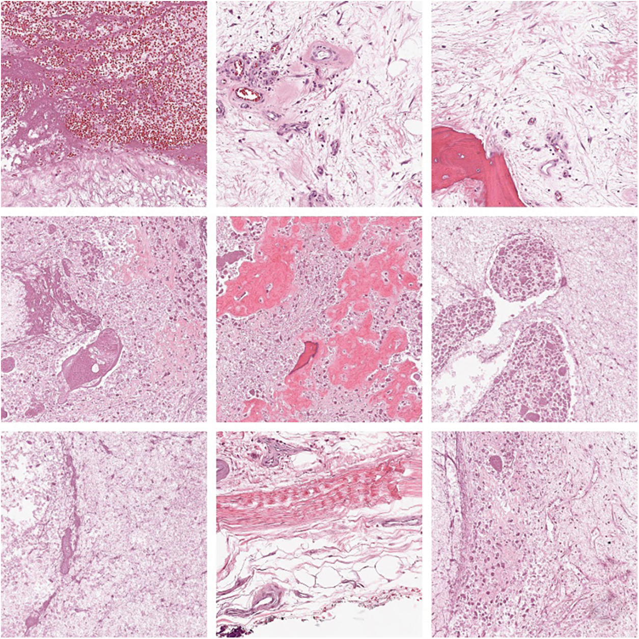
Figure 3: Sample images

Fig. 4 exhibits a set of confusion matrices generated by the proposed BOIC-EHODTL model on distinct sizes of training (TR) and testing (TS) datasets. With 70% of TR data, BOIC-EHODTL model classified 243 images into VT, 175 images into NVT, and 368 images into NT. Moreover, with 30% of TS data, the proposed BOIC-EHODTL technique categorized 96 images into VT, 83 images into NVT, and 164 images into NT. In line with this, at 80% of TR data, BOIC-EHODTL model recognized 281 images into VT, 212 images into NVT, and 397 images into NT. At last, with 20% of TS data, the proposed BOIC-EHODTL approach classified 63 images into VT, 41 images into NVT, and 122 images into NT.

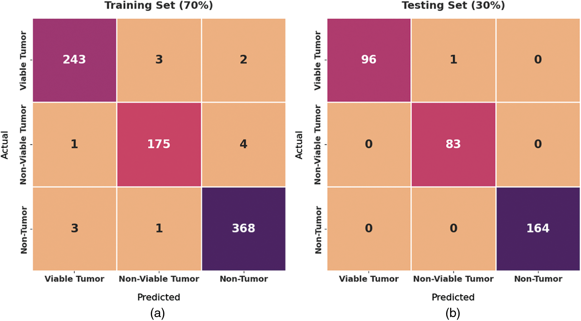
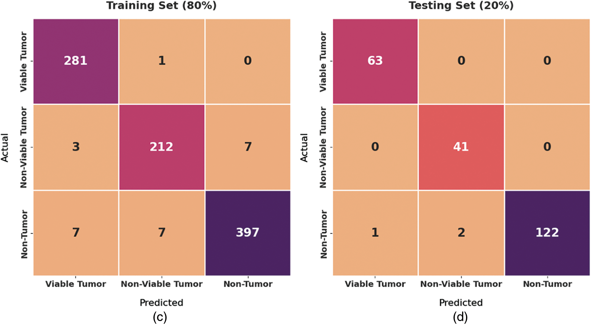
Figure 4: Confusion matrix of BOIC-EHODTL technique on distinct TR and TS datasets

Fig. 5 shows the results produced by BOIC-EHODTL model on 70% of TR data. The experimental values denote that the proposed BOIC-EHODTL model showed high performance under every class. For instance, BOIC-EHODTL model identified the samples under VT class with accuy, precn, recal, specy, and Gmeasure values such as 98.88%, 98.38%, 97.98%, 99.28%, and 98.18% respectively. Along with that, BOIC-EHODTL system identified the samples as NVT class with accuy, precn, recal, specy, and Gmeasure values such as 98.88%, 97.77%, 97.22%, 99.35%, and 97.49% respectively. Moreover, the proposed BOIC-EHODTL algorithm categorized the samples under NT class with accuy, precn, recal, specy, and Gmeasure values such as 98.75%, 98.40%, 98.92%, 98.60%, and 98.66% respectively.

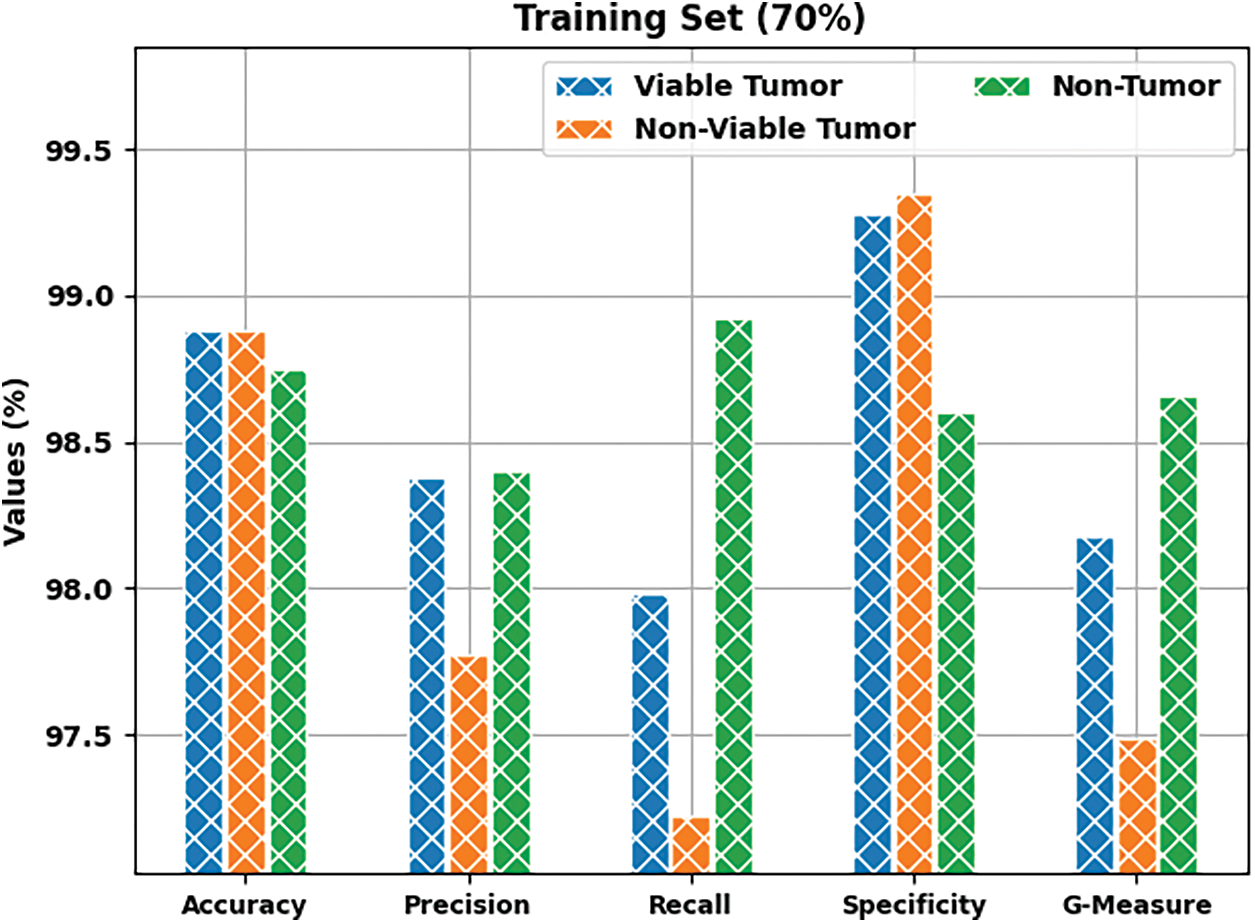
Figure 5: Results of the analysis of BOIC-EHODTL technique on 70% of TR data

Tab. 1 provides a brief overview on classifier results achieved by BOIC-EHODTL model under distinct class labels. Fig. 6 demonstrates the results accomplished by BOIC-EHODTL model on 30% of TS data. The experimental values represent that the proposed BOIC-EHODTL system increased its performance under every class. For instance, the proposed BOIC-EHODTL technique identified the samples under VT class with accuy, precn, recal, specy, and Gmeasure values such as 99.71%, 100%, 98.97%, 100%, and 99.48% correspondingly. Likewise, BOIC-EHODTL approach classified the samples under NVT class with accuy, precn, recal, specy, and Gmeasure values like 99.71%, 98.81%, 100%, 99.62%, and 99.40% correspondingly. Furthermore, BOIC-EHODTL model categorized the samples under NT class with accuy, precn, recal, specy, and Gmeasure values such as 100%, 100%, 100%, 100%, and 100% correspondingly.

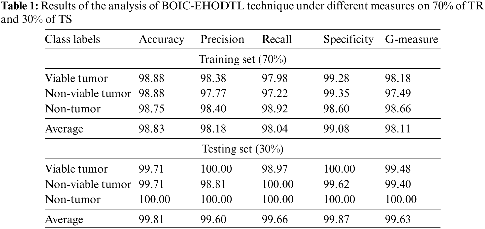
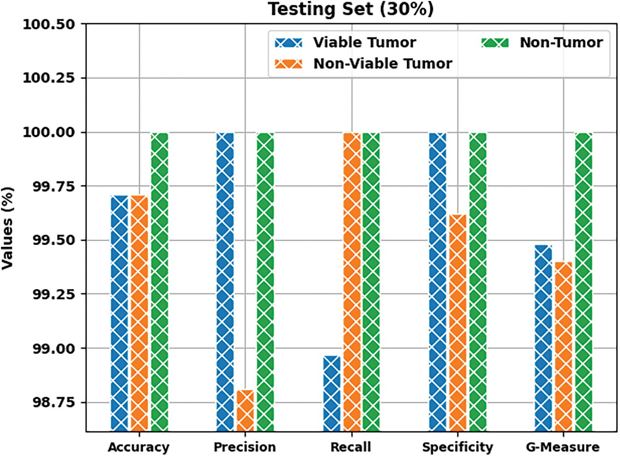
Figure 6: Results of the analysis of BOIC-EHODTL technique on 30% of TS data

Tab. 2 offers an overview on classifier results accomplished by BOIC-EHODTL technique under distinct class labels. Fig. 7 portrays the results attained by BOIC-EHODTL approach on 80% of TR data. The experimental values denote that the proposed BOIC-EHODTL methodology obtained an increased performance under every class. For instance, BOIC-EHODTL model found the samples under VT class with accuy, precn, recal, specy, and Gmeasure values such as 98.80%, 96.56%, 99.65%, 98.42%, and 98.09% respectively. Similarly, the presented BOIC-EHODTL model categorized the samples under NVT class with accuy, precn, recal, specy, and Gmeasure values such as 98.03%, 96.36%, 95.50%, 98.85%, and 95.93% correspondingly. Eventually, the proposed BOIC-EHODTL system classified the samples under NT class with accuy, precn, recal, specy, and Gmeasure values like 97.70%, 98.27%, 96.59%, 98.61%, and 97.43% respectively.

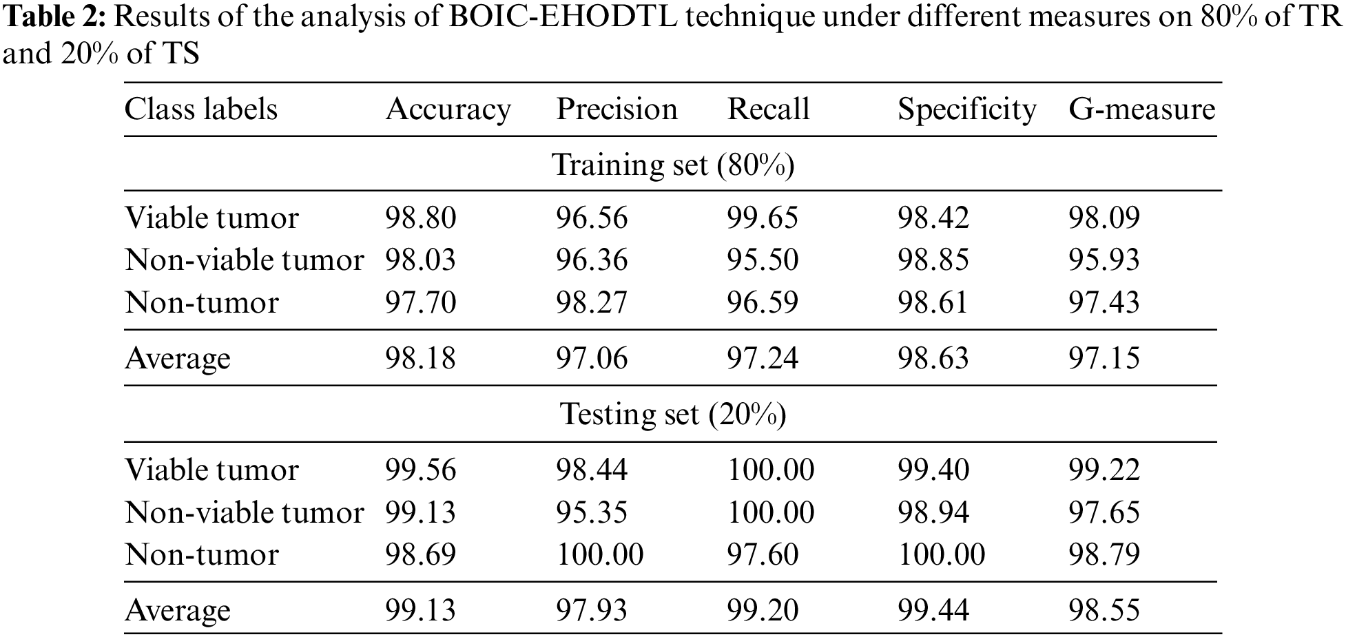
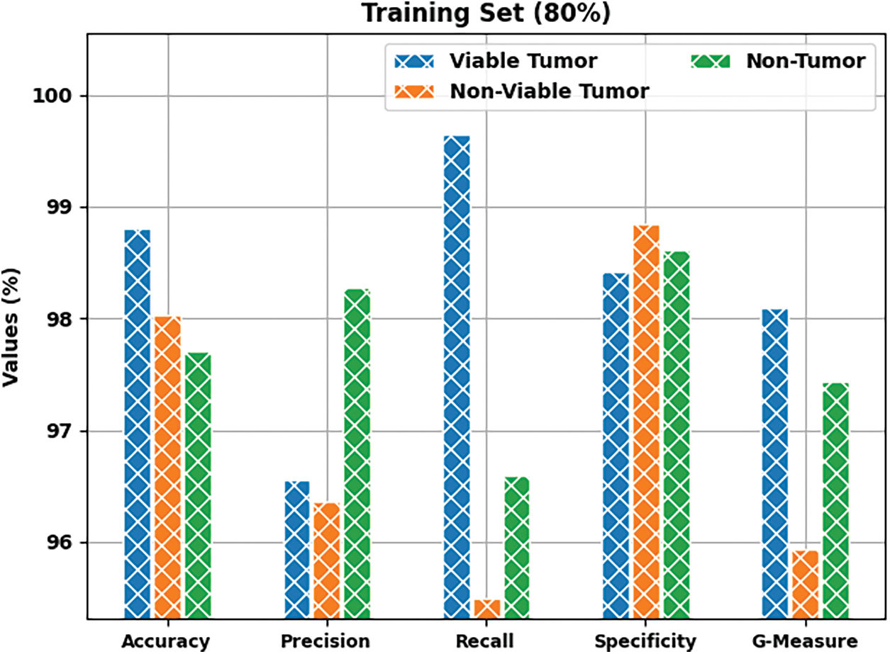
Figure 7: Results of the analysis of BOIC-EHODTL technique on 80% of TR data

Fig. 8 depicts the results accomplished by BOIC-EHODTL method on 20% of TS data. The experimental values infer that the proposed BOIC-EHODTL model achieved an increased performance under every class. For instance, BOIC-EHODTL model identified the samples under VT class with accuy, precn, recal, specy, and Gmeasure values such as 99.56%, 98.44%, 100%, 99.40%, and 99.22% respectively. Followed by, BOIC-EHODTL model classified the samples under NVT class with accuy, precn, recal, specy, and Gmeasure values such as 99.13%, 95.35%, 100%, 98.94%, and 97.65% correspondingly. In addition, BOIC-EHODTL approach categorized the samples under NT class with accuy, precn, recal, specy, and Gmeasure values such as 98.69%, 100%, 97.60%, 100%, and 98.79% correspondingly.

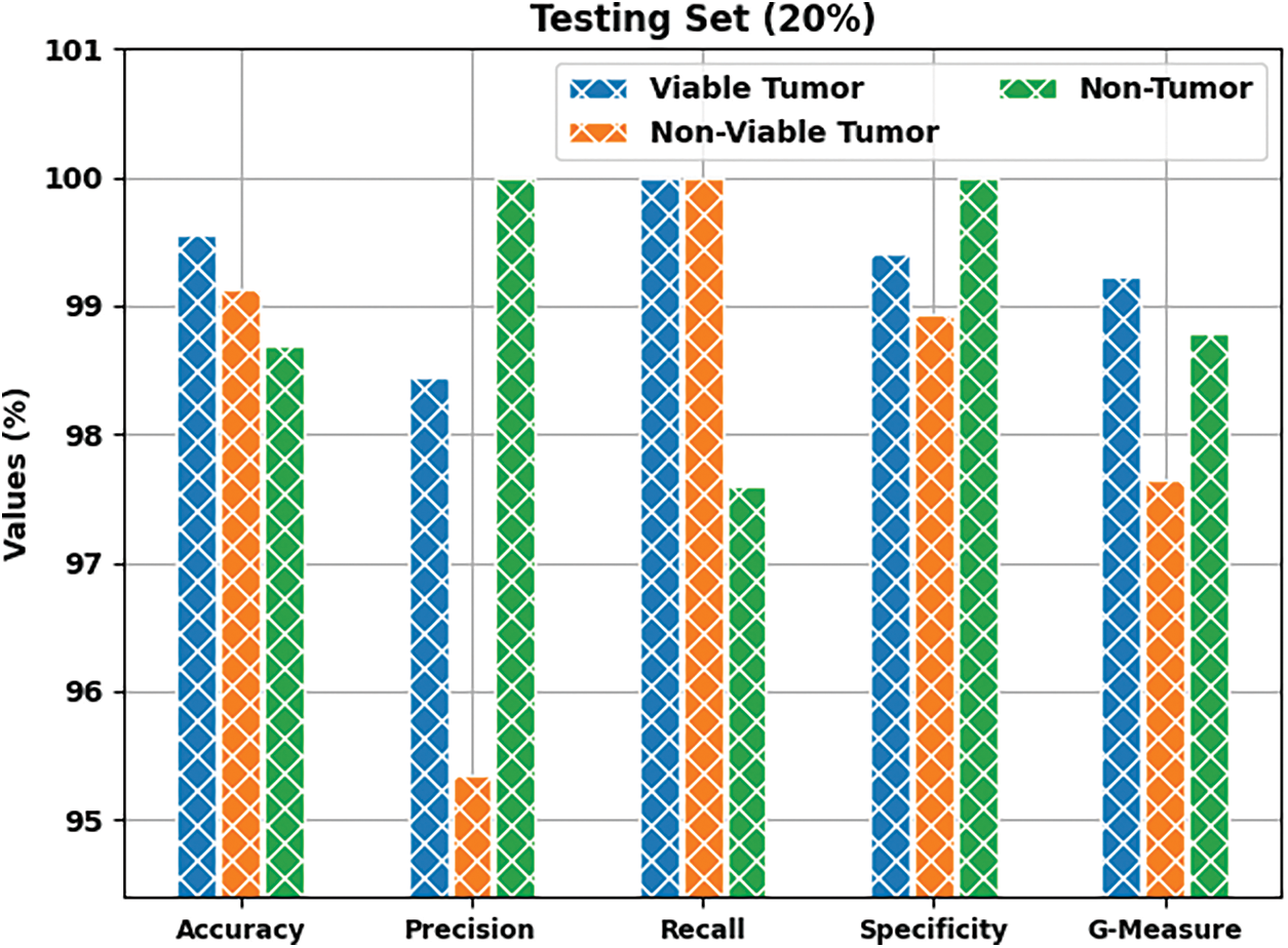
Figure 8: Results of the analysis of BOIC-EHODTL technique on 20% of TS data

Both Training Accuracy (TA) and Validation Accuracy (VA), attained by BOIC-EHODTL model on test dataset, were determined and the results are demonstrated in Fig. 9. The experimental outcomes imply that the proposed BOIC-EHODTL model achieved the maximum TA and VA values. To be specific, VA seemed to be higher than TA.

Figure 9: TA and VA analyses results of BOIC-EHODTL technique

Both Training Loss (TL) and Validation Loss (VL), achieved by the proposed BOIC-EHODTL model on test dataset, were determined and the results are portrayed in Fig. 10. The experimental outcomes infer that the proposed BOIC-EHODTL model accomplished the least TL and VL values. To be specific, VL seemed to be lower than TL.

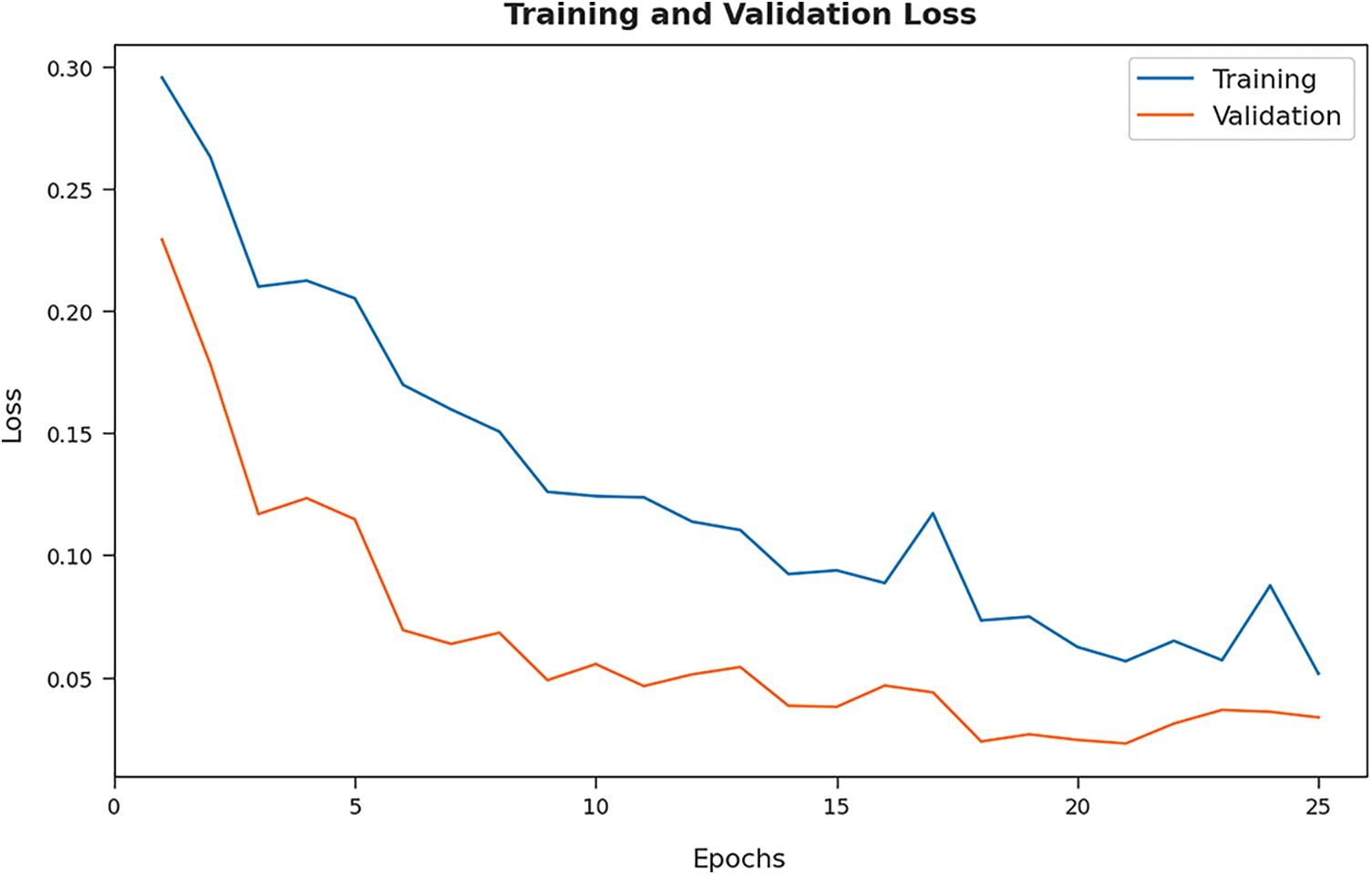
Figure 10: TL and VL analyses results of BOIC-EHODTL technique

Tab. 3 offers the comparison study results between BOIC-EHODTL model and other models. Fig. 11 shows the accuy values obtained by BOIC-EHODTL model and other recent models. The figure shows that Support Vector Machine (SVM) model achieved ineffectual results with a minimal accuy of 89.90%. In line with this, CNN, DL, and Visual Geometry Group (VGG)-19 models reached moderate accuy values such as 92.40%, 91.20%, and 93.91% respectively. Along with that, Xception model accomplished a reasonably accuy of 99.54%. But the proposed BOIC-EHODTL model produced the maximum accuy of 99.81%.

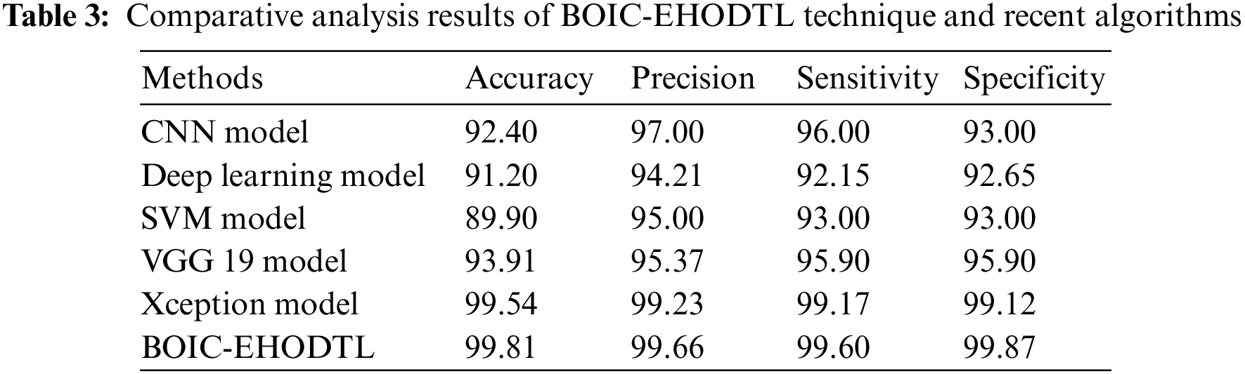
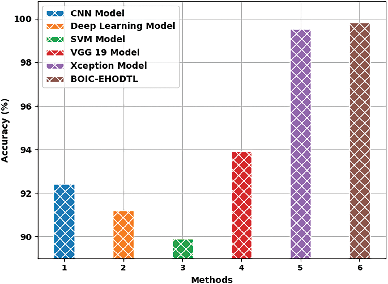
Figure 11: Accy analysis results of BOIC-EHODTL technique and other recent algorithms

Fig. 12 shows the precn values obtained by the proposed BOIC-EHODTL model and other recent models. The figure highlights that SVM model resulted in ineffectual outcomes with a minimal precn value of 95%. Eventually, CNN, DL, and VGG-19 systems reached moderately closer precn values such as 97%, 94.21%, and 95.37% respectively. In addition, Xception model accomplished a reasonable precn of 99.23%. However, the proposed BOIC-EHODTL technique produced the highest precn of 99.66%.

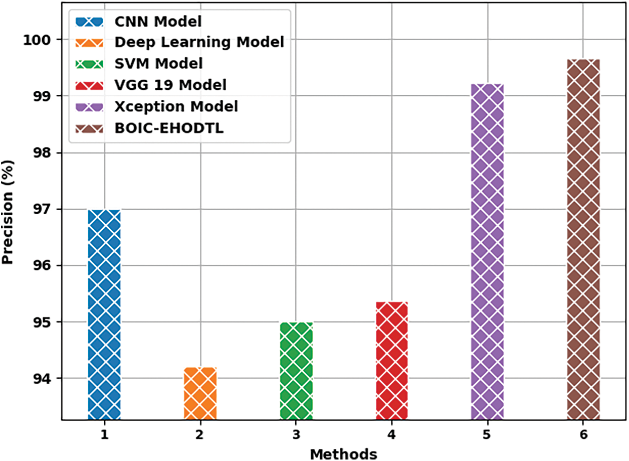
Figure 12: Precn analysis results of BOIC-EHODTL technique and other recent algorithms

Fig. 13 portrays the sensy values obtained by BOIC-EHODTL model and other recent models. The figure highlights that SVM model produced ineffectual results with a minimal sensy value of 93%. Besides, CNN, DL, and VGG-19 algorithms reached moderately closer sensy values such as 96%, 92.15%, and 95.90% respectively. Similarly, Xception model accomplished a reasonable sensy of 99.17%. At last, the proposed BOIC-EHODTL methodology produced a high sensy of 99.60%. From the detailed results and discussion, it is apparent that BOIC-EHODTL model is superior to recent models under different measures.

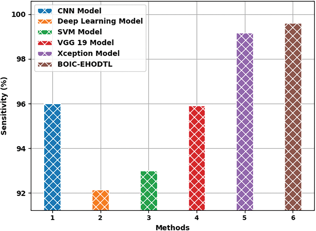
Figure 13: Sensy analysis results of BOIC-EHODTL technique and other recent algorithms

4  Conclusion

In this study, a novel BOIC-EHODTL model has been developed to analyze biomedical images and identify distinct kinds of osteosarcoma. Primarily, GF technique is employed as a pre-processing technique to get rid of the noise from images. At the same time, Adam optimizer with MixNet model is also employed as a feature extraction technique to generate feature vectors. Moreover, EHO algorithm with ANFC model is utilized for both recognition and categorization of osteosarcoma. EHO algorithm is used to fine tune the parameters involved in ANFC model. In order to demonstrate the improved performance of BOIC-EHODTL model, a comprehensive comparison analysis was conducted upon benchmark dataset and the results portrayed better performance of BOIC-EHODTL model over recent methodologies. In future, hybrid DL models can be employed in the classification of other biomedical images too.

Funding Statement: The authors extend their appreciation to the Deanship of Scientific Research at King Khalid University for funding this work through Large Groups Project under grant number (42/43). Princess Nourah bint Abdulrahman University Researchers Supporting Project number (PNURSP2022R151), Princess Nourah bint Abdulrahman University, Riyadh, Saudi Arabia. The authors would like to thank the Deanship of Scientific Research at Umm Al-Qura University for supporting this work by Grant Code: (22UQU4340237DSR16).

Conflicts of Interest: The authors declare that they have no conflicts of interest to report regarding the present study.

References

 1.  D. M. Anisuzzaman, H. Barzekar, L. Tong, J. Luo and Z. Yu, “A deep learning study on osteosarcoma detection from histological images,” Biomedical Signal Processing and Control, vol. 69, no. 5, pp. 102931, 2021. [Google Scholar]

 2.  S. Mahore, K. Bhole and S. Rathod, “Machine learning approach to classify and predict different osteosarcoma types,” in 2021 8th Int. Conf. on Signal Processing and Integrated Networks (SPIN), Noida, India, pp. 641–645, 2021. [Google Scholar]

 3.  W. Wang, X. Huang, J. Li, P. Zhang and X. Wang, “Detecting COVID-19 patients in X-ray images based on MAI-nets,” International Journal of Computational Intelligence Systems, vol. 14, no. 1, pp. 1607–1616, 2021. [Google Scholar]

 4.  Y. Gui and G. Zeng, “Joint learning of visual and spatial features for edit propagation from a single image,” The Visual Computer, vol. 36, no. 3, pp. 469–482, 2020. [Google Scholar]

 5.  W. Wang, Y. T. Li, T. Zou, X. Wang, J. Y. You et al., “A novel image classification approach via Dense-MobileNet models,” Mobile Information Systems, 2020. [Google Scholar]

 6.  S. R. Zhou, J. P. Yin and J. M. Zhang, “Local binary pattern (LBP) and local phase quantization (LBQ) based on Gabor filter for face representation,” Neurocomputing, vol. 116, no. 6 (June), pp. 260–264, 2013. [Google Scholar]

 7.  Y. Song, D. Zhang, Q. Tang, S. Tang and K. Yang, “Local and nonlocal constraints for compressed sensing video and multi-view image recovery,” Neurocomputing, vol. 406, no. 2, pp. 34–48, 2020. [Google Scholar]

 8.  D. Zhang, S. Wang, F. Li, S. Tian, J. Wang et al., “An efficient ECG denoising method based on empirical mode decomposition, sample entropy, and improved threshold function,” Wireless Communications and Mobile Computing, vol. 2020, no. 2, pp. 1–11, 2020. [Google Scholar]

 9.  X. R. Zhang, X. Sun, W. Sun, T. Xu and P. P. Wang, “Deformation expression of soft tissue based on BP neural network,” Intelligent Automation & Soft Computing, vol. 32, no. 2, pp. 1041–1053, 2022. [Google Scholar]

10. X. R. Zhang, W. F. Zhang, W. Sun, X. M. Sun and S. K. Jha, “A robust 3-D medical watermarking based on wavelet transform for data protection,” Computer Systems Science & Engineering, vol. 41, no. 3, pp. 1043–1056, 2022. [Google Scholar]

11. R. Liu, D. Pan, Y. Xu, H. Zeng, Z. He et al., “A deep learning-machine learning fusion approach for the classification of benign, malignant, and intermediate bone tumors,” European Radiology, vol. 32, no. 2, pp. 1371–1383, 2022. [Google Scholar]

12. B. C. Mohan, “Osteosarcoma classification using multilevel feature fusion and ensembles,” in 2021 IEEE 18th India Council Int. Conf. (INDICON), Guwahati, India, pp. 1–6, 2021. [Google Scholar]

13. S. J. Badashah, S. S. Basha, S. R. Ahamed and S. P. V. Subba Rao, “Fractional-harris hawks optimization-based generative adversarial network for osteosarcoma detection using renyi entropy-hybrid fusion,” International Journal of Intelligent Systems, vol. 36, no. 10, pp. 6007–6031, 2021. [Google Scholar]

14. H. Bansal, B. Dubey, P. Goyanka and S. Varshney, “Assessment of osteogenic sarcoma with histology images using deep learning,” in Machine Learning and Information Processing, Advances in Intelligent Systems and Computing Book Series. Vol. 1311. Singapore: Springer, pp. 215–223, 2021. [Google Scholar]

15. A. A. Malibari, R. Alshahrani, F. N. Al-Wesabi, S. B. Haj Hassine, M. A. Alkhonaini et al., “Artificial intelligence based prostate cancer classification model using biomedical images,” Computers, Materials & Continua, vol. 72, no. 2, pp. 3799–3813, 2022. [Google Scholar]

16. R. Poonia, M. Gupta, I. Abunadi, A. A. Albraikan, F. N. Al-Wesabi et al., “Intelligent diagnostic prediction and classification models for detection of kidney disease,” Healthcare, vol. 10, no. 2, pp. 371, 2022. [Google Scholar]

17. A. S. Almasoud, S. B. Haj Hassine, F. N. Al-Wesabi, M. K. Nour, A. M. Hilal et al., “Automated multi-document biomedical text summarization using deep learning model,” Computers, Materials & Continua, vol. 71, no. 3, pp. 5799–5815, 2022. [Google Scholar]

18. Y. Wang, J. Yan, Z. Yang, Y. Zhao and T. Liu, “Optimizing GIS partial discharge pattern recognition in the ubiquitous power internet of things context: A MixNet deep learning model,” International Journal of Electrical Power & Energy Systems, vol. 125, no. 4, pp. 106484, 2021. [Google Scholar]

19. Z. Zhang, “Improved adam optimizer for deep neural networks,” in 2018 IEEE/ACM 26th Int. Symp. on Quality of Service (IWQoS), Banff, AB, Canada, pp. 1–2, 2018. [Google Scholar]

20. J. Rawat, A. Singh, H. S. Bhadauria, J. Virmani and J. S. Devgun, “Leukocyte classification using adaptive neuro-fuzzy inference system in microscopic blood images,” Arabian Journal for Science and Engineering, vol. 43, no. 12, pp. 7041–7058, 2018. [Google Scholar]

21. K. Shankar, E. Perumal, M. Elhoseny, F. Taher, B. B. Gupta et al., “Synergic deep learning for smart health diagnosis of COVID-19 for connected living and smart cities,” ACM Transactions on Internet Technology, vol. 22, no. 3, pp. 1–14, 2022. [Google Scholar]

22. K. Shankar, E. Perumal, V. G. Díaz, P. Tiwari, D. Gupta et al., “An optimal cascaded recurrent neural network for intelligent COVID-19 detection using Chest X-ray images,” Applied Soft Computing, vol. 113, no. Part A, pp. 1–13, 2021. [Google Scholar]

23. K. Shankar, E. Perumal, P. Tiwari, M. Shorfuzzaman and D. Gupta, “Deep learning and evolutionary intelligence with fusion-based feature extraction for detection of COVID-19 from chest X-ray images,” Multimedia Systems, vol. 66, no. 2, pp. 1921, 2021. [Google Scholar]

24. K. Shankar and E. Perumal, “A novel hand-crafted with deep learning features based fusion model for COVID-19 diagnosis and classification using chest X-ray images,” Complex & Intelligent Systems, vol. 7, pp. 1277–1293, 2020. [Google Scholar]

25. J. Li, H. Lei, A. H. Alavi and G. G. Wang, “Elephant herding optimization: Variants, hybrids, and applications,” Mathematics, vol. 8, no. 9, pp. 1415, 2020. [Google Scholar]

26. P. Leavey, A. Sengupta, D. Rakheja, O. Daescu, H. B. Arunachalam et al., “Osteosarcoma data from UT Southwestern/UT Dallas for viable and necrotic tumor assessment,” [Data set] The Cancer Imaging, 2019. https://wiki.cancerimagingarchive.net/pages/viewpage.action?pageId=52756935 [Google Scholar]

This work is licensed under a Creative Commons Attribution 4.0 International License, which permits unrestricted use, distribution, and reproduction in any medium, provided the original work is properly cited.