Computers, Materials & Continua DOI:10.32604/cmc.2022.031425
Article

Water Wave Optimization with Deep Learning Driven Smart Grid Stability Prediction

Anwer Mustafa Hilal1,2,*, Aisha Hassan Abdalla Hashim1, Heba G. Mohamed3, Mohammad Alamgeer4,5, Mohamed K. Nour6, Anas Abdelrahman7 and Abdelwahed Motwakel2

1Department of Electrical and Computer Engineering, International Islamic University Malaysia, Kuala Lumpur, 53100, Malaysia
2Department of Computer and Self Development, Preparatory Year Deanship, Prince Sattam Bin Abdulaziz University, AlKharj, Saudi Arabia
3Department of Electrical Engineering, College of Engineering, Princess Nourah Bint Abdulrahman University, P.O. Box 84428, Riyadh, 11671, Saudi Arabia
4Department of Information Systems, College of Science & Art at Mahayil, King Khalid University, Saudi Arabia
5Department of Computer Science and Bioinformatics, Singhania University, Pacheri Bari, Jhnujhunu, Rajasthan, India
6Department of Computer Sciences, College of Computing and Information System, Umm Al-Qura University, Saudi Arabia
7Department of Mechanical Engineering, Faculty of Engineering & Technology, Future University in Egypt, New Cairo, 11835, Egypt
*Corresponding Author: Anwer Mustafa Hilal. Email: a.hilal@psau.edu.sa
Received: 17 April 2022; Accepted: 29 May 2022

Abstract: Smart Grid (SG) technologies enable the acquisition of huge volumes of high dimension and multi-class data related to electric power grid operations through the integration of advanced metering infrastructures, control systems, and communication technologies. In SGs, user demand data is gathered and examined over the present supply criteria whereas the expenses are then informed to the clients so that they can decide about electricity consumption. Since the entire procedure is valued on the basis of time, it is essential to perform adaptive estimation of the SG’s stability. Recent advancements in Machine Learning (ML) and Deep Learning (DL) models enable the designing of effective stability prediction models in SGs. In this background, the current study introduces a novel Water Wave Optimization with Optimal Deep Learning Driven Smart Grid Stability Prediction (WWOODL-SGSP) model. The aim of the presented WWOODL-SGSP model is to predict the stability level of SGs in a proficient manner. To attain this, the proposed WWOODL-SGSP model initially applies normalization process to scale the data to a uniform level. Then, WWO algorithm is applied to choose an optimal subset of features from the pre-processed data. Next, Deep Belief Network (DBN) model is followed to predict the stability level of SGs. Finally, Slime Mold Algorithm (SMA) is exploited to fine tune the hyperparameters involved in DBN model. In order to validate the enhanced performance of the proposed WWOODL-SGSP model, a wide range of experimental analyses was performed. The simulation results confirm the enhanced predictive results of WWOODL-SGSP model over other recent approaches.

Keywords: Smart grid; stability prediction; deep learning; energy systems; machine learning; metaheursitics

1  Introduction

Renewable Energy (RE) is a much-needed, cleaner and greener substitute for fossil fuels and it has achieved tremendous growth in recent years [1]. Before the arrival of RE, power utilities and other types of production centers supply electricity to end users through conventional grids. This conventional method is characterized by unidirectional flows between energy provider and the end-user. But, the increasing penetration of RE brought the concept of ‘prosumer’ in which both the energy is supplied as well as consumed by the end users [2]. It needs a bi-directional flow of energy in grids. The arrival of such ‘prosumers’ and increasing preference for RE involves complex energy concepts in terms of generation, allocation and dissipation. Economic effects associated with this phenomena are too complicate to address and challenging to overcome especially, whether to buy or not the energy supplied at the offered rate [3]. Related endowments on tackling the needs of such a new phenomenon have been provided by both academia and industries in the past few years. There has been significant amount of studies conducted in the domain of Smart Grid (SG) stability [4].

The durability of electrical grids is decided by the balance between demand and generation of the electricity [5]. Traditional power systems can achieve this balancing factor via demand-led electrical power production. Due to the progressive movement from fossil-related power generation to RE resources, grid topology has become decentralized and energy flow has become bi-directional. In other terms, end users might function as both consumers as well as producers simultaneously and are frequently termed as ‘prosumers’ [6]. The fluctuating nature and unstable character of RE resources pose an important problem with regards to design plans and control upon electric power grid. To create a balance between demand and supply in these fluctuating power grids, numerous SG methods have been suggested earlier. The main concept applied is the regulation of end user’s demand which is generally referred to as ‘demand response’ technique [7]. Demand response can be defined by the alterations in the dissipation of electrical power, in comparison with usual patterns of dissipation, by end users in response to the alterations in electrical power rate.

Data Mining (DM) methods are highly appropriate for decision making process in stability analysis management as well as in controlling the power systems that involve decentralization of SGs [8]. This is attributed to the fact that there exists huge volumes of experimental data on different angles of power system operations. Many DM approaches have been utilized in the research domain which are discussed in the next section. However, its important shortcomings are generally black-box, no transparency and focus only upon accuracy. It has been found that the studies conducted earlier do not want to conduct in-depth insights or justifications and clarifications for the judgments made. Further, they do not offer any insights about the mechanism for the provided system [9]. Several DM and machine-learning algorithms have been implemented too for decentralized management and control of SGs [10].

In this background, the current research article introduces a novel Water Wave Optimization with Optimal Deep Learning Driven Smart Grid Stability Prediction (WWOODL-SGSP) model. The presented WWOODL-SGSP model initially applies normalization process to scale the data to a uniform level. Then, WWO approach is utilized to choose an optimal subset of features from the pre-processed data. Next, Deep Belief Network (DBN) model is applied to predict the stability level of SGs. Finally, Slime Mold Algorithm (SMA) is exploited for fine tuning the hyperparameters involved in DBN model. In order to establish the enhanced performance of the proposed WWOODL-SGSP model, a wide range of experimental analyses was conducted.

Rest of the paper is organized as follows. Section 2 offers information on related works, Section 3 details the proposed model, Section 4 discusses the results, and Section 5 draws the conclusion.

2  Literature Review

In literature [11], the researchers developed an enhanced short-term load prediction technique. Initially, the load is decomposed into distinct frequency modules that vary from low to high levels which is realized through an ensemble empirical-mode decomposition approach. Next, the smooth and periodic low-frequency component is forecasted through a multi-variable linear regression model while preserving the effective computational ability. Mazhari et al. [12] addressed an original technique to predict the rotor angle stability in power system. In the presented architecture, a Fault Cluster (FC) theory was presented to divide the electrical network into disparate zones. FC is defined as per the installed PMU location in such a way that the powerful fault detection module can identify the source of fault in the network amongst FCs.

In the study conducted earlier [13], a Long Short Term Memory (LSTM), Recurrent Neural Network (RNN) was utilized for demand forecasting and electricity price using big data. The researchers actively worked to present a novel model for forecasting. This model contains multiple and single input variables. In the study, the researchers witnessed that the usage of multiple variables enhances prediction performance. Ghadimi et al. [14] presented a novel hybrid prediction method named as Multi-Stage Forecast Engine (MSFE) and dual-tree complex wavelet transform. In this method, a signal is entered to propose the wavelet transform. Later, it is filtrated with the help of novel feature selection. Next, the signal is forecasted by the presented model. An intelligent technique was employed in this study to predict the engine capability in terms of increasing its performance.

Huang et al. [15] presented a novel technology named Elman Neural Network (ENN)-driven Wavelet Transform (WT-ENN) to forecast the hourly solar irradiance. Zhu et al. [16] developed a hierarchical DL machine (HDLM) for effectively accomplishment of qualitative and quantitative online Transient Stability Prediction (TSP). To enhance the online efficacy, multiple generator fault-on trajectories along with two closest datapoints in pre-or post-fault phases were attained using PMU to form a raw input. Muralitharan et al. [17] presented a NN-based optimization method to predict the energy demands. Convolutional Neural Network (CNN) method was applied in this study to estimate the energy demand at user end.

3  The Proposed Model

In this study, a new WWOODL-SGSP model is proposed to predict the stability level of SGs in a proficient manner. At first, the proposed WWOODL-SGSP model employs normalization process to scale up the data to a uniform level. Besides, WWO approach is utilized to select an optimal subset of structures from pre-processed data. Then, DBN method is applied to predict the stability level in SGs. Finally, SMA algorithm is exploited for fine tuning the hyperparameters involved in DBN model. Fig. 1 illustrates the block diagram of WWOODL-SGSP technique.

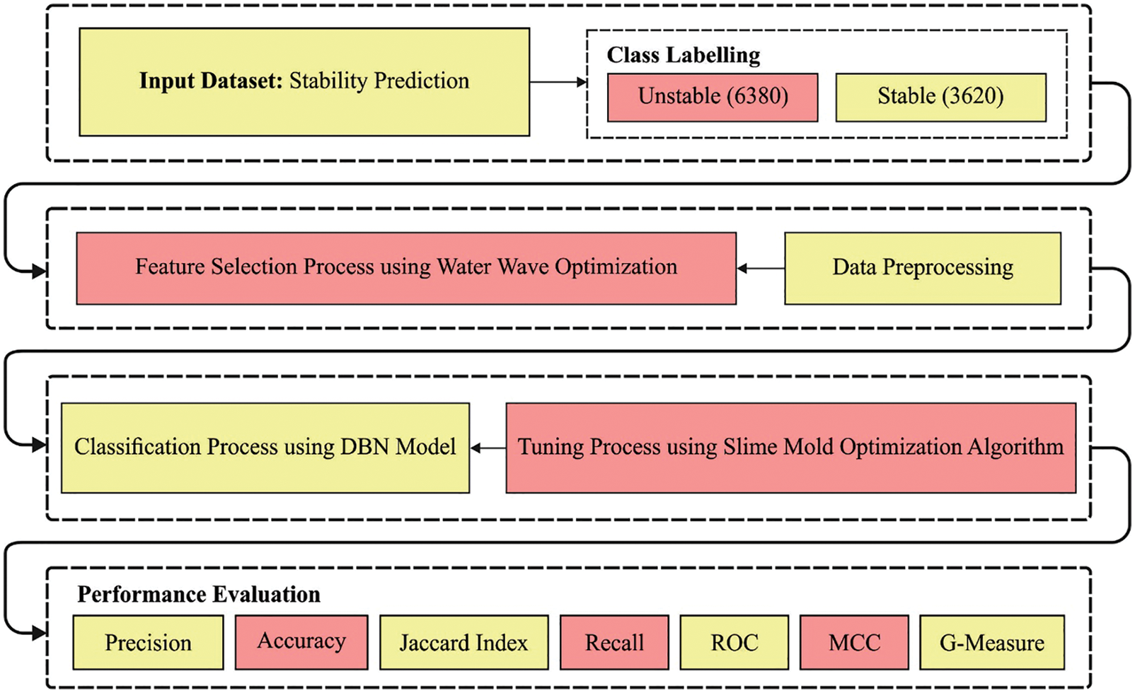
Figure 1: Block diagram of WWOODL-SGSP technique

3.1 Data Preprocessing

At the initial stage, the proposed WWOODL-SGSP model employs normalization process to scale up the data to a uniform level. In order to transform the actual data into a uniform format, data normalization is required. In this case, min-max normalization method is used to transform the data into a uniform range of 0 and1. It can be expressed as follows.

Y=Yoriginal−YminYmax−Ymin(1)

whereas Yoriginal signifies the input value of y feature, Ymin represents the minimal value of y feature, and Ymax denotes the superior value of y feature.

3.2 Feature Selection Using WWO Algorithm

Once the input data is pre-processed, WWO approach is utilized to choose an optimal subset of features from the pre-processed data [18]. WWO is an enhanced version of shallow WW methodology and is used to resolve optimization issues. Without any loss in generalization issue, an increasing problem occurs in the objective function, f. WWO algorithm has three different operations such as Breaking, Propagation and Refraction. For every generation, a wave should be forwarded precisely.

u′(d)=u(d)+ran(−1,1)⋅λL(d)(2)

whereas L(d) describe the length of dth dimensional vector (1≤d≤n), and ran indicates an arbitrary value within (−1,1). For every case, the wavelength of every wave u can be expanded with the help of the given function.

λ=λ⋅α−(f(x)−fmn+ε)/(f mx −fm1π+ε)(3)

Here, α represents the wavelength decreasing coefficients, e displays n minimum positive units to remove the divisible value by 0 and f mx  and f mn  denote the maximal and minimal fitness values from current population.

3.2.1 Refraction

In this method, refraction on wave is calculated by restricting the height to 0, and implies a simple model to determine the location after the completion of refraction method.

u′(d)=N(u∗(d)+u(d)2,|u∗(d)−u(d)|2)(4)

where u∗ displays the best outcomes, N(µ,σ) indicates a Gaussian random value with mean µ and SD σ. Novel location is an arbitrary value that is partially centered around original position along with optimal position whereas SD is the same original value of differences.

λ′=λf(u)f(u′)(5)

3.2.2 Breaking

Whenever a wave shifts from a position where the depth of water is minimal than the prevailing value, wave crest velocity exceeds wave celerity. At last, a crest is highly efficient and the wave is classified into pieces as ‘one single wave’. Further, k dimensions are randomly selected while the dimension d produces a single wave u′ as given in the following equation.

u′(d)=u(d)+N(0,1)⋅βL(d)(6)

Now, β denotes the breaking coefficient. In the absence of lonely waves, then the possible values become u∗. Then, u∗ is applied whereas it is latter is swapped with an efficient one from the lonely waves. WWO-FS technique intends to exploit the optimal set of features on input data to achieve high accuracy at less number of features. It can be integrated into an individual weighted indicator whereas identical fitness function can be employed as given below.

fitness=ω1×acc(classifier)+ω2×(1−sp)(7)

where p defines the total feature count and s implies the chosen feature count. The acc(classifer) denotes the accuracy offered by DBN model as provided below.

acc(classifier)=ncnc+ni×100% )(8)

where ni and nc define the inaccurately- and accurately-classified instance count. Fig. 2 illustrates the steps involved in WWO technique.

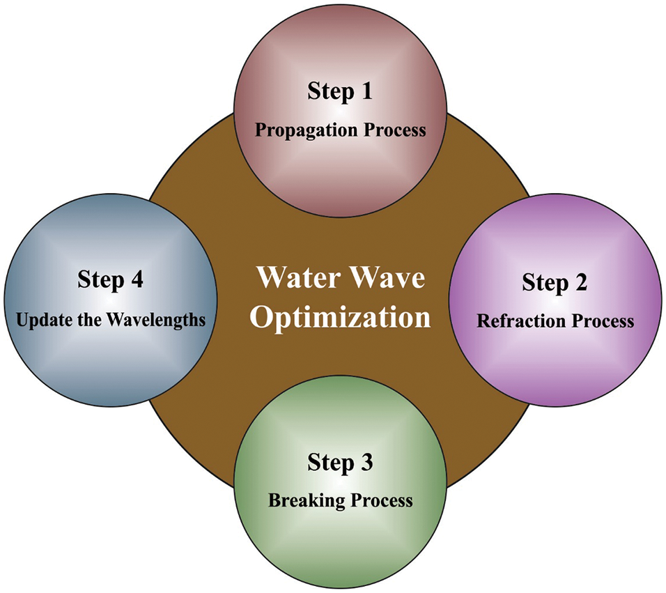
Figure 2: Steps in WWO technique

3.3 Stability Prediction Model

In this stage, DBN model is applied to predict the stability level of SGs [19]. RNN is commonly employed in time series datasets for prediction purposes. Generally, NN with multiple layers is called as Deep Neural Network (DNN). It is challenging to achieve accurate DNN models based on Backpropagation (BP) method. So, different learning methodologies have been developed earlier which are equivalent to DNN such as dropout and pre-training. There are different approaches used in DNN namely CNN, DBN, and so on. In DBN, several RBMs are organized in a layer-wise training model to resolve the optimization problem. CNN training model cannot be implemented to train multilayer networks. The training process of DBN is categorized into tuning and pre-training stages. Fig. 3 illustrates the architecture of DBN.

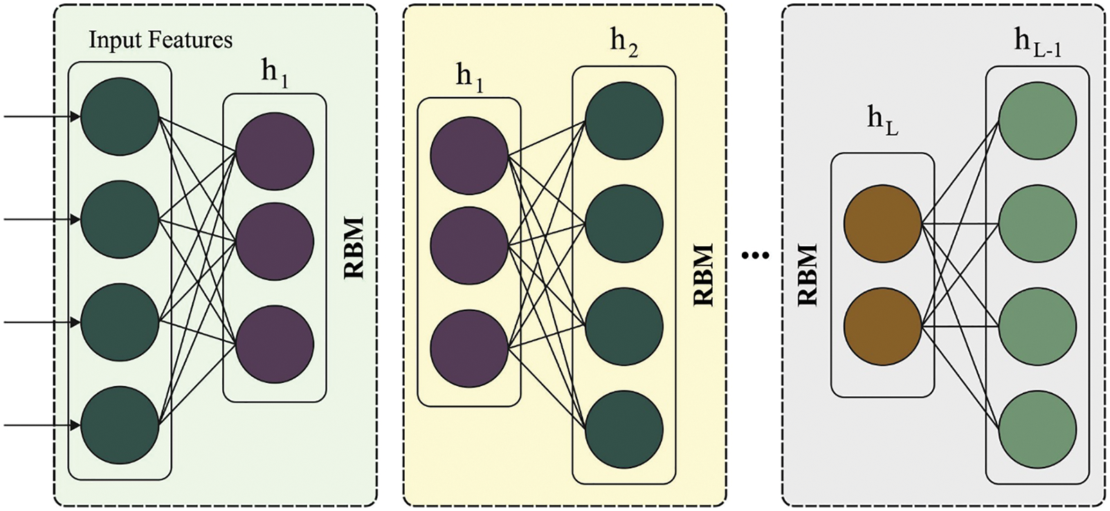
Figure 3: Structure of DBN

Being an important feed forward network and deep structure, the current study uses DBN method. Here, the sample is produced from input to output layer via hidden layer with further layers. Based on DBN, the hidden unit generates the activation functions and classifies the system on its own. Furthermore, Restricted Boltzmann Machine (RBM) is also deployed to address the problem of generating the activation function.

Next, the precise unit ν is uploaded by training RBM vector.

F(v,h)=−∑k=1K∑l=1LWklvkhl−∑k=1Kαkvk−∑l=1Lβlhl(9)

Here, Wkl indicates a programmatic interaction between the hidden unit ‘hl’ and visible unit ‘vk’. Now, α and β represent the biases while K and L denote the number of visible and hidden values. The succeeding log probability of preparation vector is concerned about the inconsistent weight. In case of hidden unit from RBM, it does not offer an instant response that could attain impartial samples from (Vk, hl) data.

ρ(hl=1|v)=δ(∑l=1LWklvk+αl)(10)

Here δ(x) denotes the logistic sigmoid function. 1(1+exp⁡(x)), while vk, hl indicate the unbiased samples.

The hidden layer is enhanced, whereas the visible unit is concurrent with visible and hidden layers.

ΔWklθ(vkhl)data−(vkhl)reconstruction(11)

Here, the RBM is trained well. Being a unique RBM, it is stacked with a frame using multi-layer model. Once the input visible unit is arranged as a vector, the quality of unit is effectively developed with the help of RBM layer. The distributed method is used to distribute the layers under current biases and weights. Therefore, the attained DNN weight is embedded during fine-tuning stage.

3.4 Hyperparameter Optimization

In this final stage, SMA algorithm is exploited for fine tuning the hyperparameters involved in DBN model [20]. SMA is a metaheuristic method inspired by the capability of a single cell organism i.e., slime mold to find the optimal path towards food centers through searching or exploring the optimal solutions. Here, the mathematical formulation of the slime mold nature is created whereas the succeeding rules are defined to determine the upgraded location, when searching for food. This condition is based on r and p.

X(t+1)→={Xb(t)→+vb→→⋅(W→⋅XA(t)→−XB(t)→)r<pvc→⋅X(t)→r≥p(12)

where vb→ denotes a variable that lies in [−a,a], vc→ implies a parameter that moves towards 0. ‘t’ implies the present round, Xb represents the location of all particles in area, where the odor is high, X→ implies the position of mold, X→A and X→B indicate the arbitrarily-chosen parameters from swarm, W→ denotes the weight of the slime mold. The maximal bound of p can be calculated as follows.

p=tan⁡h|S(i)−DF|(13)

whereas i∈1,2,…,n, S(i)= fitness of X→, DF=overallfitness from every step.

Here, v→b can be defined as follows.

vb→=→[−a,a](14)

a=arctan⁡h(−(tmax−t)+1)(15)

W→ can be determined as given herewith.

W(smellindex(i))→={1+r⋅log⁡(bF−S(i)bF−wF+1),condition1−r⋅log⁡(bF−S(i)bF−wF+1),others(16)

SmellIndex=sort(S)(17)

where S(i) ranks in first half population, r denotes an arbitrary value within [0,1], bF implies the optimum fitness attained in present process, Sort (s) function arranges the fitness value and wF represents the poor fitness value attained during iterative procedure. Next, the location of the agent is upgraded using Eq. (18):

X∗→={rand⋅(UB−LB)+LB,rand<zXb(t)→+vb→→⋅(W⋅XA(t)→−XB(t),→r<p,vc→⋅X(t)→r≥p(18)

Here, LB and UB denote the searching bounds and r denotes the arbitrary value. Finally, by upgrading the searching procedure, vb→ value arbitrarily alters between [−a,a] and vc→ that lies on [−1, 1] and it finally reaches zero which is termed as ‘food grabbing process’.

In this case, SMA technique is executed for fine tuning the hyperparameters involved in BiGRU technique by minimized MSE. It can be determined as follows.

MSE=1T∑j=1L∑i=1M(yji−dji)2(19)

Here, M and L demonstrate the outcome values of layer and data correspondingly, and yji and dji indicate the reached and appropriate magnitudes for jth unit in the outcome layer of network from time, t.

4  Performance Validation

In this subsection, the proposed WWOODL-SGSP model was experimentally validated using a dataset [21] that comprises of 10,000 samples with 13 features. Here, WWO-FS model selected a total of eight features. The dataset includes 6,380 samples under unstable class and 3,620 samples under stable class. The feature names are tau1, tau2, tau3, tau4, p1, p2, p3, p4, g1, g2, g3, g4, and stab.

Fig. 4 shows the correlation matrix of the attributes involved in the dataset. Fig. 5 illustrates a set of confusion matrices generated by the proposed WWOODL-SGSP model on test dataset and varying epochs. The results imply that the proposed WWOODL-SGSP model categorized the data under distinct class labels. For instance, with 200 epochs, WWOODL-SGSP model recognized 6330 samples as unstable class and 3425 samples as stable class. Meanwhile, with 600 epochs, the proposed WWOODL-SGSP method categorized 6,303 samples under unstable class and 3,473 samples under stable class. Eventually, with 1200 epochs, the presented WWOODL-SGSP approach recognized 6324 samples as unstable class and 3444 samples as stable class.

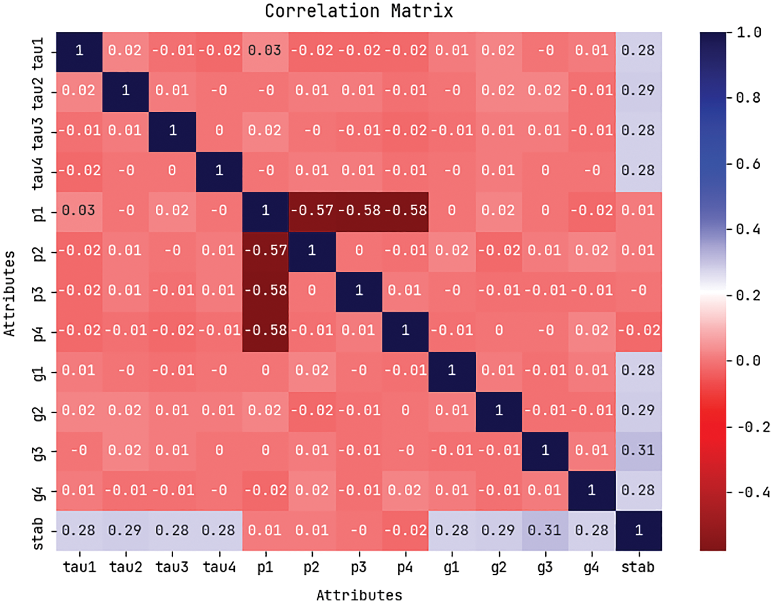
Figure 4: Correlation matrix of WWOODL-SGSP technique

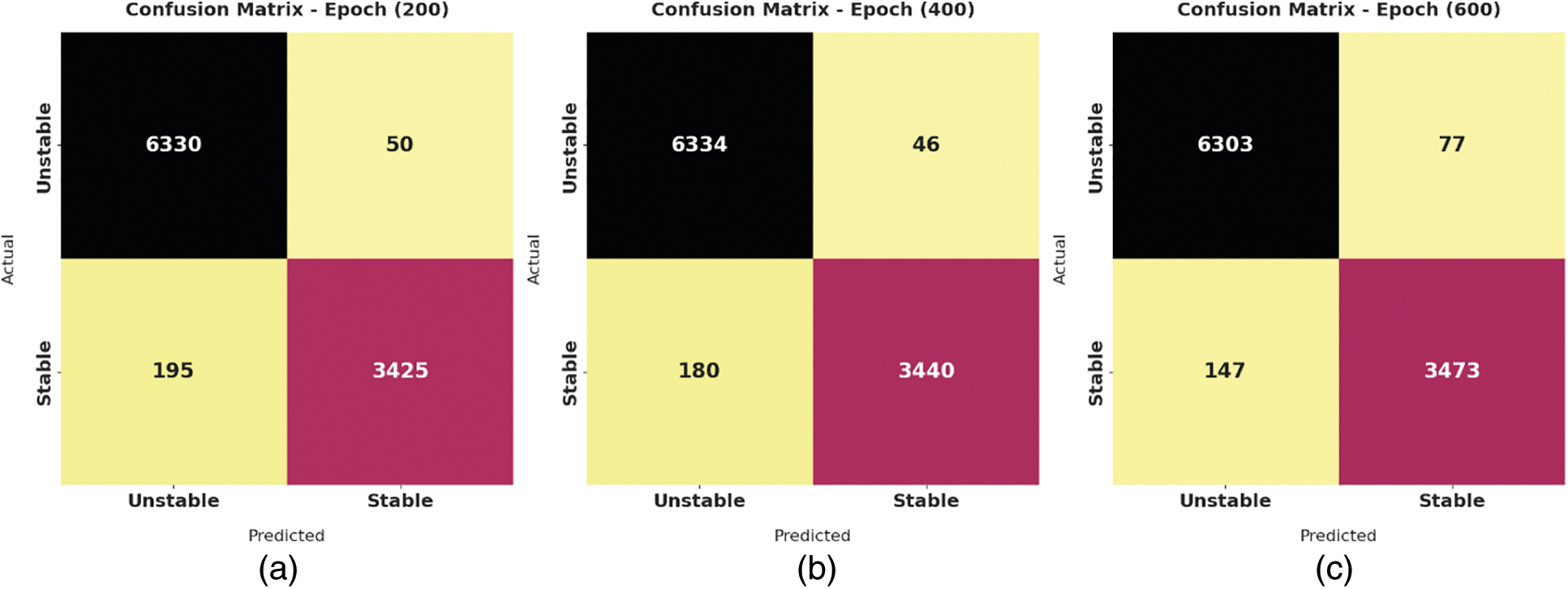
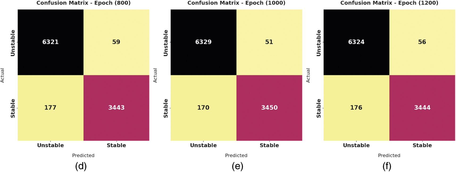
Figure 5: Confusion matrix generated by WWOODL-SGSP technique under distinct epochs

Tab. 1 and Fig. 6 highlight the overall classification results achieved by the proposed WWOODL-SGSP model under distinct epochs. The experimental values infer that WWOODL-SGSP model produced enhanced classification performance over other models. For instance, with 200 epochs, the proposed WWOODL-SGSP model attained accuy, precn, recal, MCC, Gmeasure, and Jaccard Index values such as 97.55%, 97.79%, 96.91%, 94.70%, 97.34%, and 94.80% respectively. Along with that, with 400 epochs, the proposed WWOODL-SGSP method reached accuy, precn, recal, MCC, Gmeasure, and Jaccard Index values such as 97.74%, 97.96%, 97.15%, 95.11%, 97.54%, and 95.20% correspondingly. Moreover, with 800 epochs, the presented WWOODL-SGSP model attained accuy, precn, recal, MCC, Gmeasure, and Jaccard Index values such as 97.64%, 97.80%, 97.09%, 94.89%, 97.44%, and 94.99% correspondingly. Furthermore, with 1000 epochs, the proposed WWOODL-SGSP algorithm gained accuy, precn, recal, MCC, Gmeasure, and Jaccard Index values such as 97.79%, 97.96%, 97.25%, 95.21%, 97.60%, and 95.30% respectively. At last, with 1200 epochs, the proposed WWOODL-SGSP system attained accuy, precn, recal, MCC, Gmeasure, and Jaccard Index values such as 97.68%, 97.85%, 97.13%, 94.97%, 97.48%, and 95.08% correspondingly.

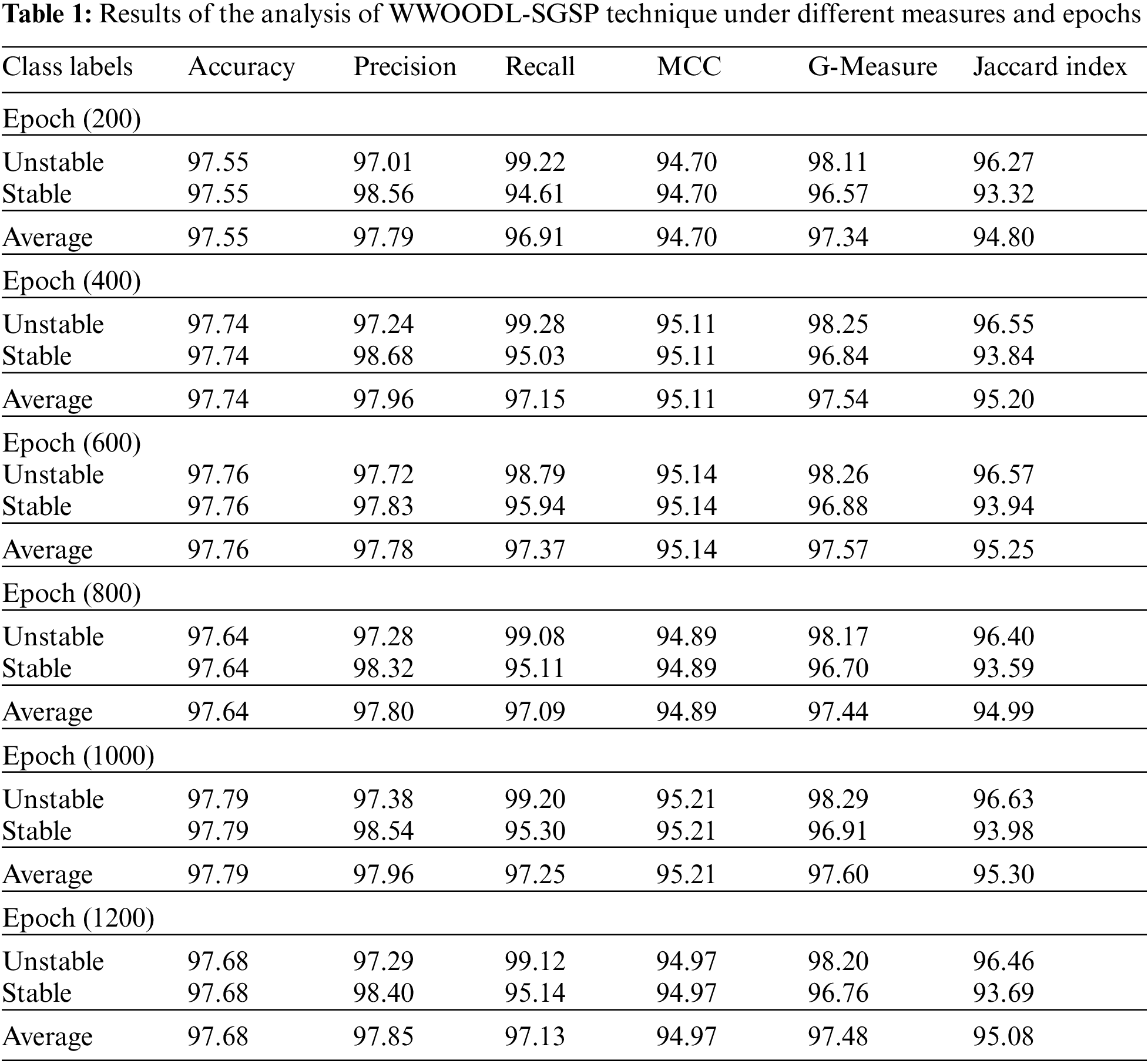
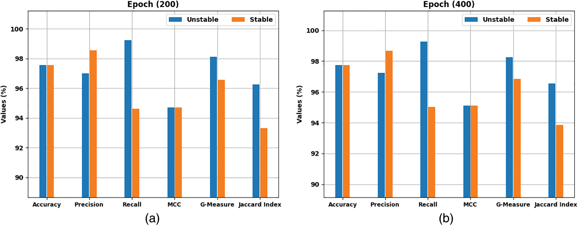
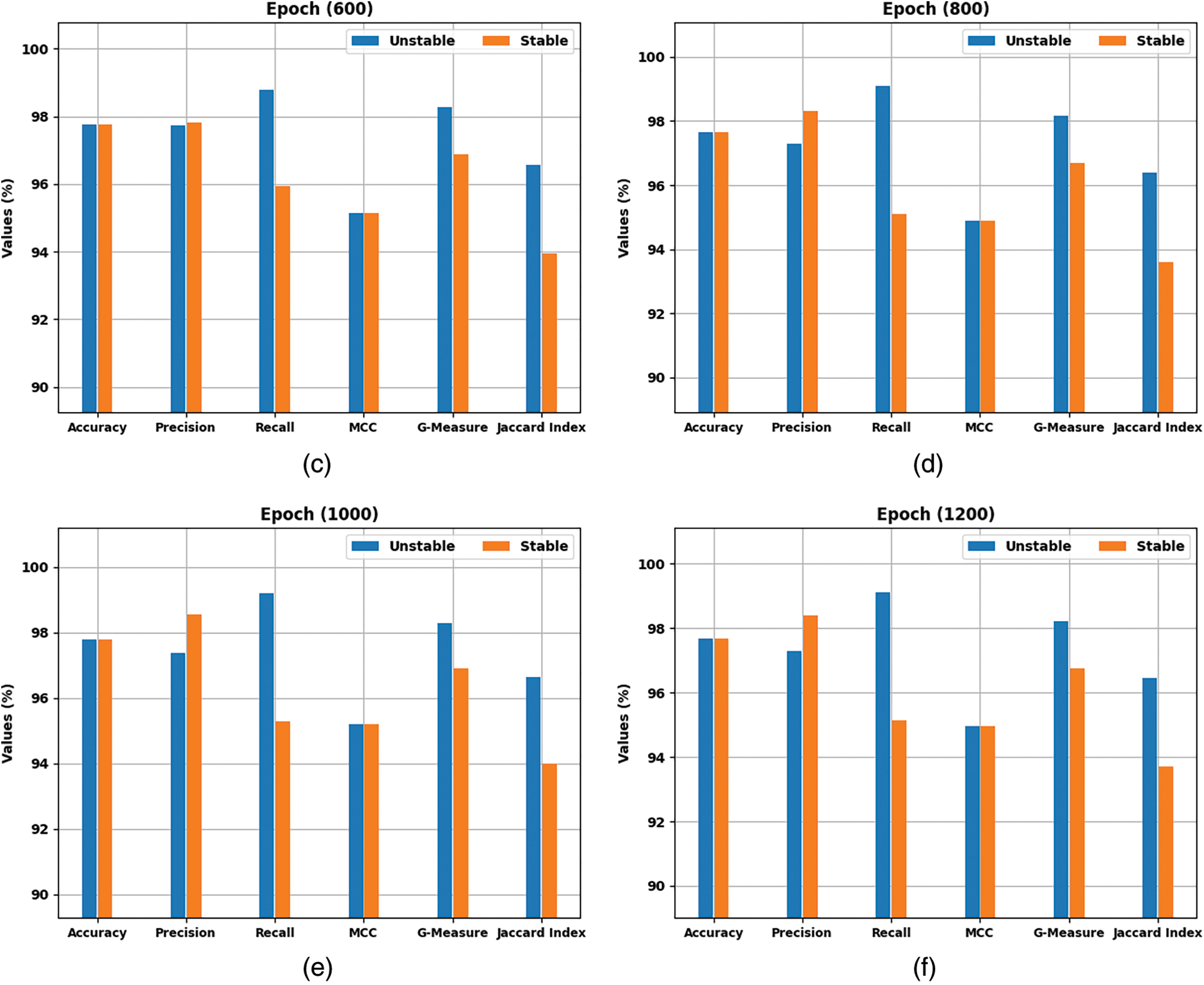
Figure 6: Results of the analysis of WWOODL-SGSP technique under different measures

Training Accuracy (TA) and Validation Accuracy (VA) values, attained by the proposed WWOODL-SGSP model on test dataset, are demonstrated in Fig. 7. The experimental outcomes infer that the proposed WWOODL-SGSP model gained the maximum TA and VA values. To be specific, VA value seemed to be higher than TA.

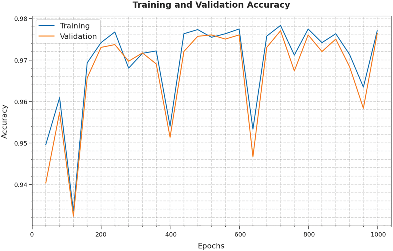
Figure 7: TA and VA analyses results of WWOODL-SGSP technique

Both Training Loss (TL) and Validation Loss (VL) values, achieved by the proposed WWOODL-SGSP model on test dataset, are shown in Fig. 8. The experimental outcomes imply that WWOODL-SGSP model accomplished the least TL and VL values. Specifically, VL seemed to be lower than TL.

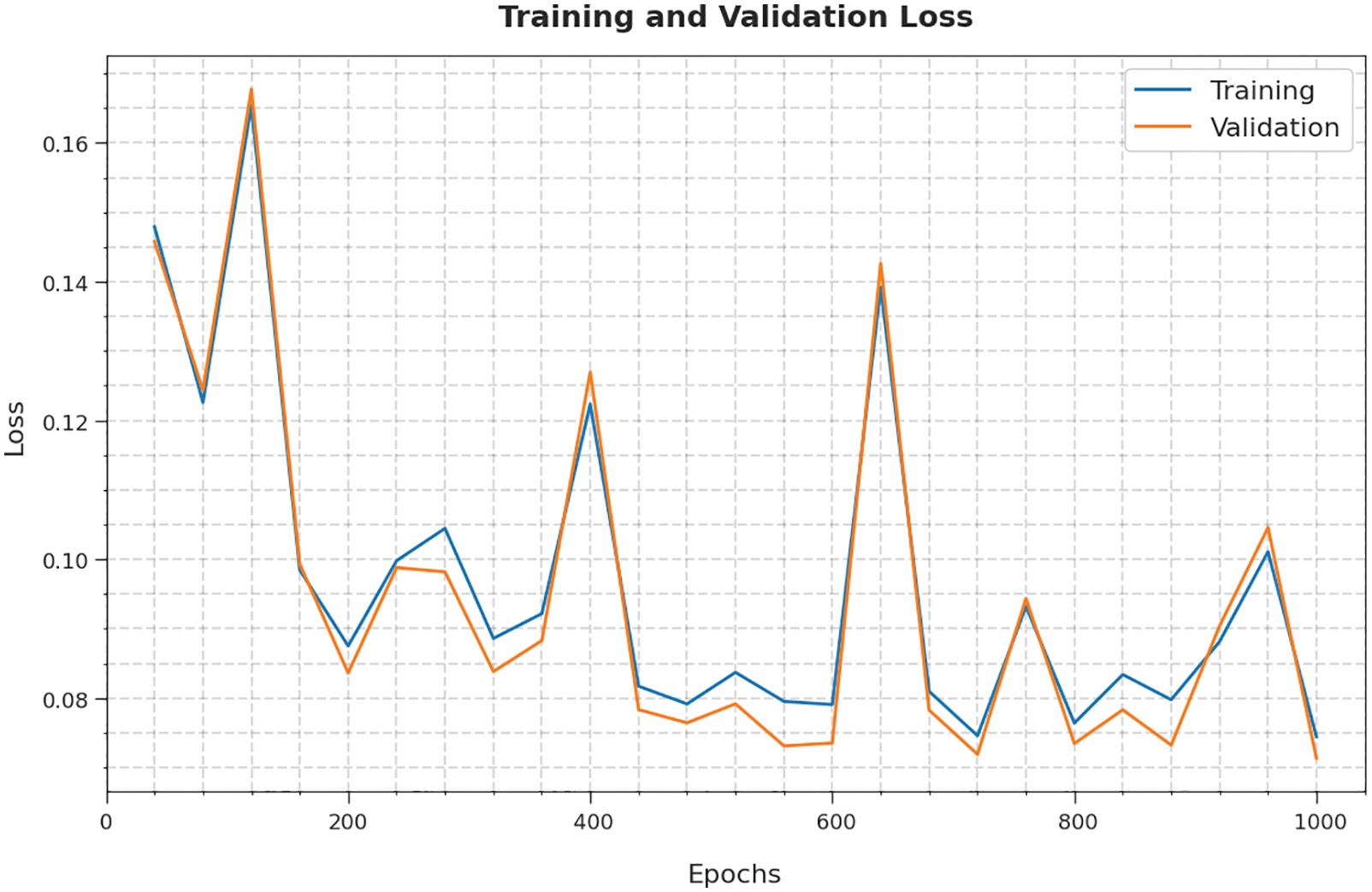
Figure 8: TL and VL analyses results of WWOODL-SGSP technique

A brief precision-recall curve analysis was conducted upon WWOODL-SGSP model on test dataset and the result is portrayed in Fig. 9. By observing the figure, it can be understood that WWOODL-SGSP model accomplished the maximum precision-recall performance under all classes.

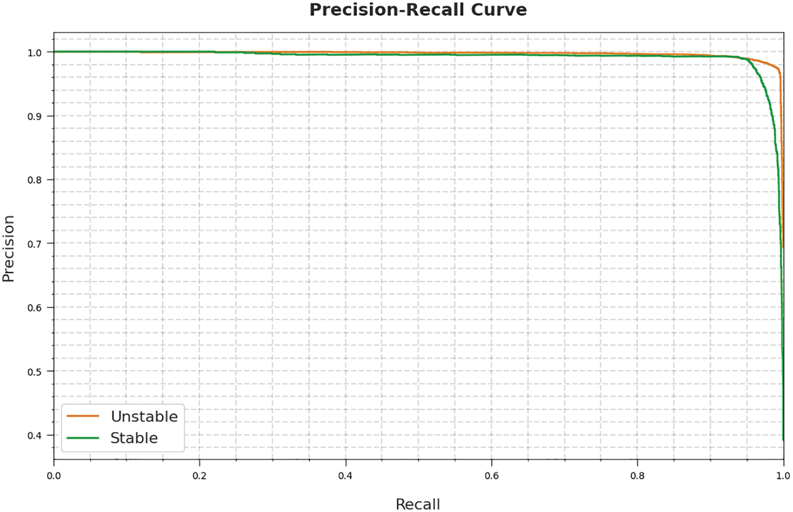
Figure 9: Precision-recall curve analysis results of WWOODL-SGSP technique

A detailed ROC curve analysis was conducted upon WWOODL-SGSP model on test dataset and the result is portrayed in Fig. 10. The result indicate that the proposed WWOODL-SGSP method exhibited its capability in categorizing two different classes such as unstable and stable on the test datasets.

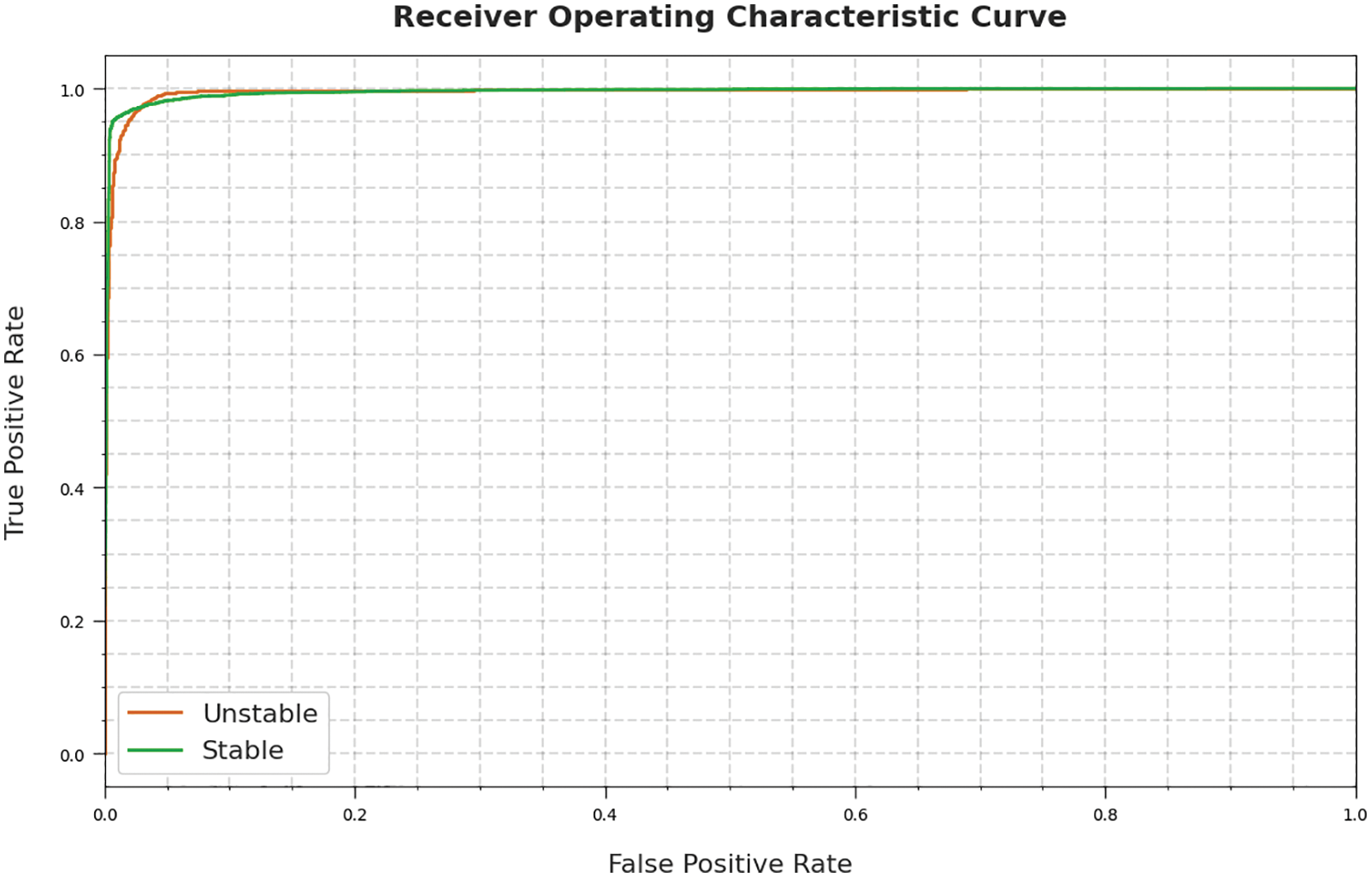
Figure 10: ROC curve analysis of WWOODL-SGSP technique

Finally, a detailed comparative accuracy analysis was conducted between WWOODL-SGSP model and other recent models and the results are shown in Tab. 2 and Fig. 11 [22]. The experimental values indicate that CART model produced the least accuracy of 79.50%. At the same time, Decision Tree (C4.5) and DL models accomplished closer accuracy values such as 89.80% and 88.72% respectively. Followed by, Bayesian optimization and XGBoost models resulted in reasonable accuracy values such as 91.10% and 97.20% respectively. However, the proposed WWOODL-SGSP model accomplished the maximum accuracy of 97.79%. From the detailed results and discussion, it can be inferred that the proposed WWOODL-SGSP model accomplished the maximum stability prediction performance on SGs.

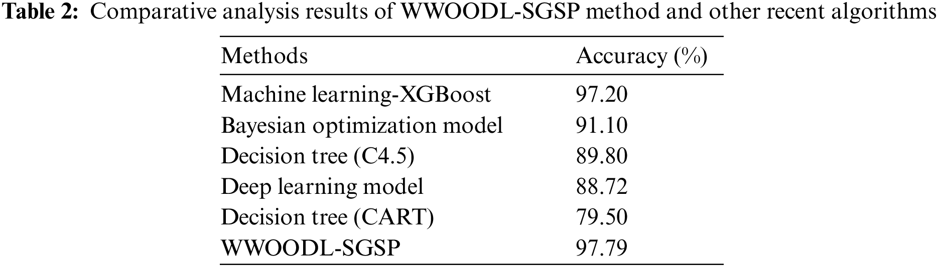
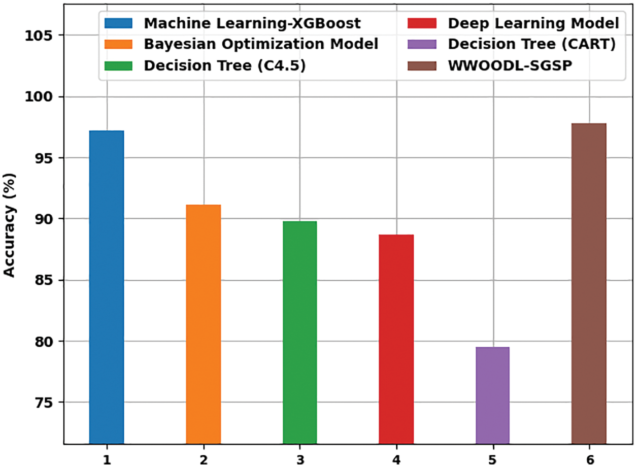
Figure 11: Comparative analysis results of WWOODL-SGSP model and other recent algorithms

5  Conclusion

In this study, a new WWOODL-SGSP model has been introduced to predict the stability level of SGs in a proficient manner. Initially, the proposed WWOODL-SGSP model employs normalization process to scale up the data to a uniform level. Besides, WWO algorithm is also utilized to choose an optimal subset of features from the pre-processed data. Then, DBN model is employed to predict the stability level in SGs. At the final stage, SMA algorithm is exploited for fine tuning the hyperparameters involved in DBN model. In order to exhibit the superior performance of the proposed WWOODL-SGSP model, a wide range of experimental analyses was conducted. The simulation results established the supreme prediction results of WWOODL-SGSP model over other recent approaches. In future, WWOODL-SGSP approach can be extended with the help of hybrid DL techniques.

Funding Statement: The authors extend their appreciation to the Deanship of Scientific Research at King Khalid University for funding this work through Large Groups Project under grant number (180/43). Princess Nourah bint Abdulrahman University Researchers Supporting Project number (PNURSP2022R140), Princess Nourah bint Abdulrahman University, Riyadh, Saudi Arabia. The authors would like to thank the Deanship of Scientific Research at Umm Al-Qura University for supporting this work by Grant Code: (22UQU4310373DSR23).

Conflicts of Interest: The authors declare that they have no conflicts of interest to report regarding the present study.

References

 1.  A. Shamisa, B. Majidi and J. C. Patra, “Sliding-window-based real-time model order reduction for stability prediction in smart grid,” IEEE Transactions on Power Systems, vol. 34, no. 1, pp. 326–337, 2018. [Google Scholar]

 2.  A. K. Bashir, S. Khan, B. Prabadevi, N. Deepa, W. S. Alnumay et al., “Comparative analysis of machine learning algorithms for prediction of smart grid stability,” International Transactions on Electrical Energy Systems, vol. 31, no. 9, pp. e12706, 2021. [Google Scholar]

 3.  B. S. England and A. T. Alouani, “Real time voltage stability prediction of smart grid areas using smart meters data and improved Thevenin estimates,” International Journal of Electrical Power & Energy Systems, vol. 122, no. 3, pp. 106189, 2020. [Google Scholar]

 4.  Z. Shi, W. Yao, Z. Li, L. Zeng, Y. Zhao et al., “Artificial intelligence techniques for stability analysis and control in smart grids: Methodologies, applications, challenges and future directions,” Applied Energy, vol. 278, no. 2015, pp. 115733, 2020. [Google Scholar]

 5.  Y. Zhang, T. Huang and E. F. Bompard, “Big data analytics in smart grids: A review,” Energy Informatics, vol. 1, no. 1, pp. 8, 2018. [Google Scholar]

 6.  T. Ahmad, H. Zhang and B. Yan, “A review on renewable energy and electricity requirement forecasting models for smart grid and buildings,” Sustainable Cities and Society, vol. 55, no. 1, pp. 102052, 2020. [Google Scholar]

 7.  F. Darbandi, A. Jafari, H. Karimipour, A. Dehghantanha, F. Derakhshan et al., “Real-time stability assessment in smart cyber-physical grids: A deep learning approach,” IET Smart Grid, vol. 3, no. 4, pp. 454–461, 2020. [Google Scholar]

 8.  S. Azad, F. Sabrina and S. Wasimi, “Transformation of smart grid using machine learning,” in 2019 29th Australasian Universities Power Engineering Conf. (AUPEC), Nadi, Fiji, pp. 1–6, 2019. [Google Scholar]

 9.  M. R. Chen, G. Q. Zeng, K. D. Lu and J. Weng, “A two-layer nonlinear combination method for short-term wind speed prediction based on ELM, ENN, and LSTM,” IEEE Internet of Things Journal, vol. 6, no. 4, pp. 6997–7010, 2019. [Google Scholar]

10. T. Ahmad, R. Madonski, D. Zhang, C. Huang and A. Mujeeb, “Data-driven probabilistic machine learning in sustainable smart energy/smart energy systems: Key developments, challenges, and future research opportunities in the context of smart grid paradigm,” Renewable and Sustainable Energy Reviews, vol. 160, no. 1, pp. 112128, 2022. [Google Scholar]

11. J. Li, D. Deng, J. Zhao, D. Cai, W. Hu et al., “A novel hybrid short-term load forecasting method of smart grid using MLR and LSTM neural network,” IEEE Transactions on Industrial Informatics, vol. 17, no. 4, pp. 2443–2452, 2021. [Google Scholar]

12. S. M. Mazhari, N. Safari, C. Y. Chung and I. Kamwa, “A hybrid fault cluster and thévenin equivalent based framework for rotor angle stability prediction,” IEEE Transactions on Power Systems, vol. 33, no. 5, pp. 5594–5603, 2018. [Google Scholar]

13. R. Khalid, N. Javaid, F. A. Al-zahrani, K. Aurangzeb, E. H. Qazi et al., “Electricity load and price forecasting using jaya-long short term memory (JLSTM) in smart grids,” Entropy, vol. 22, no. 1, pp. 10, 2019. [Google Scholar]

14. N. Ghadimi, A. Akbarimajd, H. Shayeghi and O. Abedinia, “A new prediction model based on multi-block forecast engine in smart grid,” Journal of Ambient Intelligence and Humanized Computing, vol. 9, no. 6, pp. 1873–1888, 2018. [Google Scholar]

15. X. Huang, J. Shi, B. Gao, Y. Tai, Z. Chen et al., “Forecasting hourly solar irradiance using hybrid wavelet transformation and elman model in smart grid,” IEEE Access, vol. 7, pp. 139909–139923, 2019. [Google Scholar]

16. L. Zhu, D. J. Hill and C. Lu, “Hierarchical deep learning machine for power system online transient stability prediction,” IEEE Transactions on Power Systems, vol. 35, no. 3, pp. 2399–2411, 2020. [Google Scholar]

17. K. Muralitharan, R. Sakthivel and R. Vishnuvarthan, “Neural network based optimization approach for energy demand prediction in smart grid,” Neurocomputing, vol. 273, no. 1, pp. 199–208, 2018. [Google Scholar]

18. F. Zhao, L. Zhang, J. Cao and J. Tang, “A cooperative water wave optimization algorithm with reinforcement learning for the distributed assembly no-idle flowshop scheduling problem,” Computers & Industrial Engineering, vol. 153, no. 10, pp. 107082, 2021. [Google Scholar]

19. D. A. Pustokhin, I. V. Pustokhina, P. Rani, V. Kansal, M. Elhoseny et al., “Optimal deep learning approaches and healthcare big data analytics for mobile networks toward 5G,” Computers & Electrical Engineering, vol. 95, no. 11, pp. 107376, 2021. [Google Scholar]

20. D. Dhawale, V. K. Kamboj and P. Anand, “An effective solution to numerical and multi-disciplinary design optimization problems using chaotic slime mold algorithm,” Engineering with Computers, 2021. [Google Scholar]

21. https://github.com/pcbreviglieri/data-science-smart-grid-stability. [Google Scholar]

22. P. Breviglieri, T. Erdem and S. Eken, “Predicting smart grid stability with optimized deep models,” SN Computer Science, vol. 2, no. 2, pp. 73, 2021. [Google Scholar]

This work is licensed under a Creative Commons Attribution 4.0 International License, which permits unrestricted use, distribution, and reproduction in any medium, provided the original work is properly cited.