Computers, Materials & Continua DOI:10.32604/cmc.2022.031602
Article

Two-Fold and Symmetric Repeatability Rates for Comparing Keypoint Detectors

Ibrahim El rube'*

Department of Computer Engineering, CCIT, Taif University, Taif, 21944, Saudi Arabia
*Corresponding Author: Ibrahim El rube'. Email: ibrahim.ah@tu.edu.sa
Received: 22 April 2022; Accepted: 08 June 2022

Abstract: The repeatability rate is an important measure for evaluating and comparing the performance of keypoint detectors. Several repeatability rate measurements were used in the literature to assess the effectiveness of keypoint detectors. While these repeatability rates are calculated for pairs of images, the general assumption is that the reference image is often known and unchanging compared to other images in the same dataset. So, these rates are asymmetrical as they require calculations in only one direction. In addition, the image domain in which these computations take place substantially affects their values. The presented scatter diagram plots illustrate how these directional repeatability rates vary in relation to the size of the neighboring region in each pair of images. Therefore, both directional repeatability rates for the same image pair must be included when comparing different keypoint detectors. This paper, firstly, examines several commonly utilized repeatability rate measures for keypoint detector evaluations. The researcher then suggests computing a two-fold repeatability rate to assess keypoint detector performance on similar scene images. Next, the symmetric mean repeatability rate metric is computed using the given two-fold repeatability rates. Finally, these measurements are validated using well-known keypoint detectors on different image groups with various geometric and photometric attributes.

Keywords: Repeatability rate; keypoint detector; symmetric measure; geometric transformation; scatter diagram

1  Introduction

Keypoints can be defined as the significant image features used in various applications, including image matching, registration, remote sensing, computer vision, and robot navigation [1–6]. Over the last few decades, numerous keypoint detectors have been proposed, each with its own set of characteristics, computation methods, intended applications, geometrical transformation invariance, and immunity to image artifacts. Consequently, a variety of measurements have been published in the literature to evaluate the performance of these detectors [7–13]. One of these critical metrics is the repeatability rate, which quantifies how well the keypoint detector produces the same keypoint for images taken of the same scene but with varying capturing viewpoints and conditions. The repeatability rate has been calculated using diverse interpretations and, as a result, different equations. While these measurements are derived from the same definition, the calculation criteria vary, resulting in different values when the same image set is used.

Moreover, the calculations for these measurements assume that one of the two images used to calculate the repeatability rate is a reference image that has not been altered. Usually, the first image in each group represents the reference image, while the following images exhibit increasing degrees of transformation or photometric variation, such as in [14]. However, this is not always true for other datasets used by researchers in this field, and it cannot always be guaranteed [10]. Thus, as a consequence, if the same repeatability rate calculation is performed while traversing the image order, the repeatability rate value may differ. Most often, calculations are performed on one image’s coordinates (referred to as an image domain in this paper), onto which the other image and its keypoints are projected. This paper examines this issue using repeatability rate plots and a scatter diagram. Additionally, a symmetric measure based on a two-fold repeatability rate definition is used to resolve the problem.

This article’s main aspects are:

•   A review of the most commonly used repeatability rates for keypoint detector evaluation;

•   A two-fold repeatability rate measure;

•   A scatter diagram that depicts the directional repeatability rates as a function of the size of the keypoints’ neighboring region; and,

•   A symmetric measure based on the two-fold repeatability rate for each pair of images.

This paper will be organized as follows: Section Two follows the definition of the repeatability rate with a generalized formula and discusses the most frequently used repeatability rate measures. Section Three illustrates and analyses the two-fold and symmetric repeatability rate measures. The fourth section contains detailed descriptions of the experiments and analyses of the results. Finally, in Section Five, conclusions are drawn based on the study’s findings and analysis.

2  Repeatability Rate Measurement

The repeatability rate measurement was introduced in [15] and later in [7] to assess and compare different feature detectors and keypoint detectors. For two images, Ia and Ib, the geometrical changes, such as rotation, scale, and translation, between the two images, are described by the homography matrix (H). This H matrix also maps the features (or keypoints) of the image Ia into the “domain” of image Ib. A keypoint or feature on the image Ia is said to be repeatable if it appears in the second image in nearly the same visible “scene” location as it should be. Consequently, the repeatability rate is defined as the number of repeated features within the two images divided by the number of all possible features that could be repeated. In general, the repeatability rate (R) is defined by:

R=#{repeatedfeatures}#{featuresallocatedfornormlization}%(1)

The repeatability rate has been used to compare feature detectors’ performance on images [1,7,8]. Despite their agreement on the definition in Eq. (1), the literature contains varying interpretations and equations. This can be attributed to the determination method of repeated features and the number of normalizing features. The type of distance measurement, the maximum distance for repeated features, and the image domain that hosts the calculations are all considered factors. This section will first formulate a general equation of a two-fold repeatability rate that shows how these factors affect calculations differently. The most common repeatability rates will be presented next, along with their calculations. The term “keypoint” is used instead of “feature” throughout this article since it focuses on keypoint detector measurements than other features.

2.1 Generalized Repeatability Rate Definition

Following the detection of the keypoints on both images separately, producing Ka and Kb, the first image Ia and its keypoints are projected onto the second image Ib using the H matrix, illustrated in Fig. 1. The projection of the image Ia onto the image Ib domain determines their common region where keypoints outside this region are excluded from correspondence computation. Therefore, these projections and common region can be represented as follows:

Ia′=HIa(2.a)

Ka′=HKa(2.b)

Ic=Ia′∩Ib(2.c)

where Ic is the common region between the projected image Ia′ and the second image Ib. Only the survived keypoints, Kas′ and Kbs, located in the common visible region Ic are considered for correspondence search. All these keypoints are also a subset of the original keypoints:

Kas′∈Ic;Kas′⊆Ka′(3.a)

Kbs∈Ic;Kbs⊆Kb(3.b)

The repeated keypoints, defined as KrpB(d), were found by searching the proximity of each keypoint Kbs with a projected keypoints Kas′ within a permissible region contoured by a distance (d), as illustrated in Fig. 1.

KrpB(d)={Kcr|dist(Kbs,Kas′)<d}(4.a)

where KrpB is the repeated keypoints based on the projection onto the domain of the image Ib, Kcr is the one-to-one correspondences, dist(.) is the distance measure, and d is the maximum allowable distance between keypoints to consider as repeatable. The computation of the repeated keypoints is influenced by the direction of the image and keypoints projection; therefore, another repeated keypoints’ measure defined by KrpA(d) exists. This is similar to Eqs. (2)–(4.a); however, this time, by projecting the image Ib and its keypoints Kbs into the first image domain A yields an image Ib′ with Kbs′ keypoints, the following repeated keypoints are given:

KrpA(d)={Kcr|dist(Kas,Kbs′)<d}(4.b)

Typically, the Euclidean distance metric is used to calculate the proximity of keypoints. This means that any projected keypoint is considered a candidate for matching if it lies in a disk region centered at a keypoint in its image domain with a maximum radius of d, as exampled in Fig. 1. Most of the repeatability measures in the literature are computed using either the repeatable keypoints KrpB(d)or KrpA(d) defined in Eqs. (4.a) and (4.b), respectively.

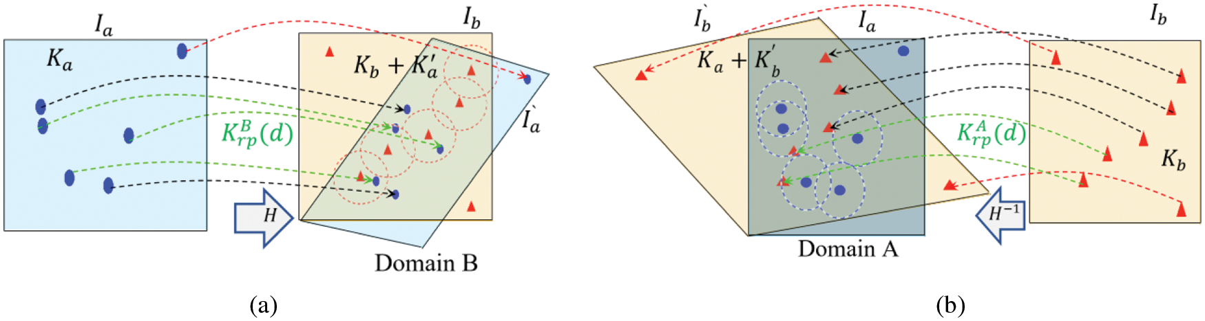
Figure 1: The repeatability is calculated either by (a) projecting the first image Ia and its keypoints Ka into the second image Ib (Domain B) using matrix H, or (b) projecting the second image Ib and its keypoints Kb into the first image Ia (Domain A) using matrix H−1. Then, the projected keypoints that fall in the d-neighbor region (dashed circles) located around the domain’s keypoints in the common visible area are used to determine repeated keypoints, which are presented by green dashed arrows and denoted by KrpA(d) and KrpB(d). Both directions have the same d value. The red dashed arrows represent keypoints projected outside the common area, while the black dashed arrows represent keypoints projected within the common area but with no correspondences

Calculating the repeatability rate may differ depending on the number of keypoints allocated (the dominator of Eq. (1). This value is used as a normalization factor to adjust the repeatability to a range of 0 to 1. As a result of the reasons mentioned above, the repeatability rate of Eq. (1) is calculated as follows:

RX(d)=NrpX(d)Nn(5)

where X is the domain in which the distance d is applied, NrpX(d)=#{KrpX(d)} is the number of repeated keypoints in the domain of image Ix, Nn is the number of the allocated keypoints that normalizes the repeatability rate measure and ensures that its upper limit equals 1. For example, if X = B and theimageIa is projected onto the domain of of the image Ib, then NrpB(d)=#{KrpB(d)}, whereas vice versa, X = A and NrpA(d)=#{KrpA(d)}. To identify a match, each keypoint’s d-neighborhood is searched for a keypoint projected from another image. The distance metric used to detect the repeating keypoints shapes the d-neighborhood around them.

The following section introduces a variety of repeatability rate definitions used in the literature to evaluate keypoint detectors and their differing interpretations of the numerators and dominators used to compute Eq. (5).

2.2 Common Repeatability Rates

The computation of the repeatability rate introduced in [7] was carried out after projecting the reference image and its features to the domain of the second image (i.e., X = B), similar to the upper graph of Fig. 1. In addition, the authors choose to normalize the repeatability by dividing it by the minimum number of features in the common visible region of the two images. Therefore, the repeatability rate concerning Eq. (5) is defined as follows:

R1B(d)=NrpB(d)min(Na′,Nb)(6.a)

where NrpB(d) is the number of repeated keypoints in the domain of the second image for d search distance. Na′=#{Kas′} is the number of the survived keypoints of the image Ia when projected to domain B, and Nb=#{Kbs} is the number of the survived keypoints of the image Ib in the same domain and same shared region Ic.

The authors of [8] calculated the repeatability; however, this was done as a function of overlapping regions. They proposed a method for calculating repeatable regions by normalizing elliptic regions between images to overcome geometric transformations such as scale change. In their work, the second image regions were projected to the first image’s domain, and then the overlay error was calculated after normalization. The repeatability of this method was found to be biased, as described in [9,16]. Furthermore, calculating the precise area of digitized elliptical regions is challenging, particularly for small sizes. The procedures in [7–9] may be appropriate for region detectors; however, for keypoint detectors, the repeatability rates using Eq. (5) are more convenient and easier to calculate because it relays more on keypoint proximity rather than overlap areas. Thus, the repeatability rate depends on computing the number of repeated keypoints and the normalizing factor dominated by the minimum number of visible keypoints in both images.

The repeatability rate of Eq. (6.a) can also be expressed in the domain of the first image:

R1A(d)=NrpA(d)min(Na,Nb′)(6.b)

where NrpA(d) is the number of repeated keypoints in the domain of the first image within the d-neighbor region, Na=#{Kas} and Nb′=#{Kbs′} represent the number of keypoints in the common area for the image Ia and the number of keypoints of the second image when projected onto domain A, respectively.

Despite being used by several authors [7, 17–19], the repeatability rate computed from Eqs. (6.a) and (6.b) has the following limitations:

•   This repeatability measurement is unreliable in terms of the effect of inter-image changes [10].

•   The minimum number of keypoints largely influences repeatability. This is especially noticeable in images with significant differences in keypoints, found in their common region, due to image scale or scene content changes [10].

•   The repeatability rate results depend on the image domain which hosts the projected keypoints.

Instead of taking the minimum value, an alternative repeatability measure proposed in [10] recommends normalizing the repeated keypoints by the average number of the survived keypoints of both images.

R2X(d)=NrpX(d)average(Na,Nb′)(7)

Although the repeatability measure, given in Eq. (7), attempted to resolve the mentioned shortcomings of the previous repeatability, its value is still dependent on the projected image domain.

Another measure, as used in [10,11], defines the repeatability rate as follows:

R3X(d)=NrpX(d)Nref(8.a)

where NrpX(d) is the number of repeated keypoints between the two images in the domain of image Ix, and Nref is the number of keypoints in the reference image that appear in the common area. The same definition has recently been applied to 3D datasets [20] and far-infrared and thermal images [21]. In [22], the authors used a similar criterion but divided by a fixed number of keypoints.

For a sequence of images, the paper in [23] demonstrated a repeatability rate for visual camera tracking that was similar to Eq. (8.a) First, the number of repeatable keypoints between two images was calculated relative to the sequence’s reference image, then divided by the number of keypoints in the first image alone.

Before performing the repeatability rate measurement described in Eq. (8.a), the authors of [17] used a “virtualized 3D scene” to pre-select the closest repeatable points in 2D and 3D spaces.

According to [12], to measure repeatability precisely, the keypoints of an image must be visible on the second image. This measurement can be performed by tracking the location of each keypoint on the images being examined using a 3D surface model. Keypoints can also be found in common regions between images, which can be used to identify them approximately. The repeatability measure used in [12]:

R3X(d)=NrpX(d)Nu(8.b)

where NrpX(d) is the number of repeated keypoints between the two images in the domain of image Ix. Nu is the number of useful keypoints of an image that appear in the common region without occlusion. Although Eq. (8.b) is more precise than Eq. (8.a), it requires manual alignment of the 3D model before applying gradient descent and simulated annealing procedures [12]. Furthermore, Eqs. (8.a) and (8.b) can obtain similar results for the non-occluded scene images; therefore, the earlier one will be used hereafter.

In [13], the repeatability rate was defined by the following:

R4X(d)=NrpX(d)2(1Na+1Nb)(9)

where Nrpx(d) is the number of repeated corners (keypoints) in image domain X, Na is the number of corners (keypoints) in the original image, and Nb is the number of corners (keypoints) in the test image. This repeatability measure is considered “average” since it uses the number of keypoints of both images to compute it. However, repeated keypoints are found only in one image domain. The definition of Eq. (9) has been used recently in the literature by several authors [6,24,25].

All the directional repeatability rates in this section are dependent on the image (domain) that hosts the computations, as shown in the plots in Fig. 2. For example, R1X(d), R2X(d), R3X(d), and R4X(d) of the two-fold repeatability rates for image groups with varying scales computed for the SURF (Speeded Up Robust Features) keypoint detector [26] are shown in Fig. 2. As in [17], in this paper, the d-neighbor distance for repeatability rates was set at d = 2.

The first group in Fig. 2, labeled “BIP,” contains images with zoom-out changes from the group’s first image, while the second, labeled “Venice,” contains zoom-in changes from the group’s reference image. The blue lines, for example, represent the repeatability rates for the image group “BIP,” with the zoom-out scale changing when calculations are performed on the first image domain, A. In contrast, the orange lines represent the repeatability rates for the same images but when computing the repeatability according to the domain of the other image. The other image group, “Venice,” exhibits zoom-in variation with gray colored lines for image domain A and yellow lines for domain B. The results, detailed in Fig. 2, confirm the repeatability rates dependency on the image domain where the distance is calculated. Therefore, a two-fold repeatability rate measure, inclusive of both calculation directions, is preferred for a pair of images.

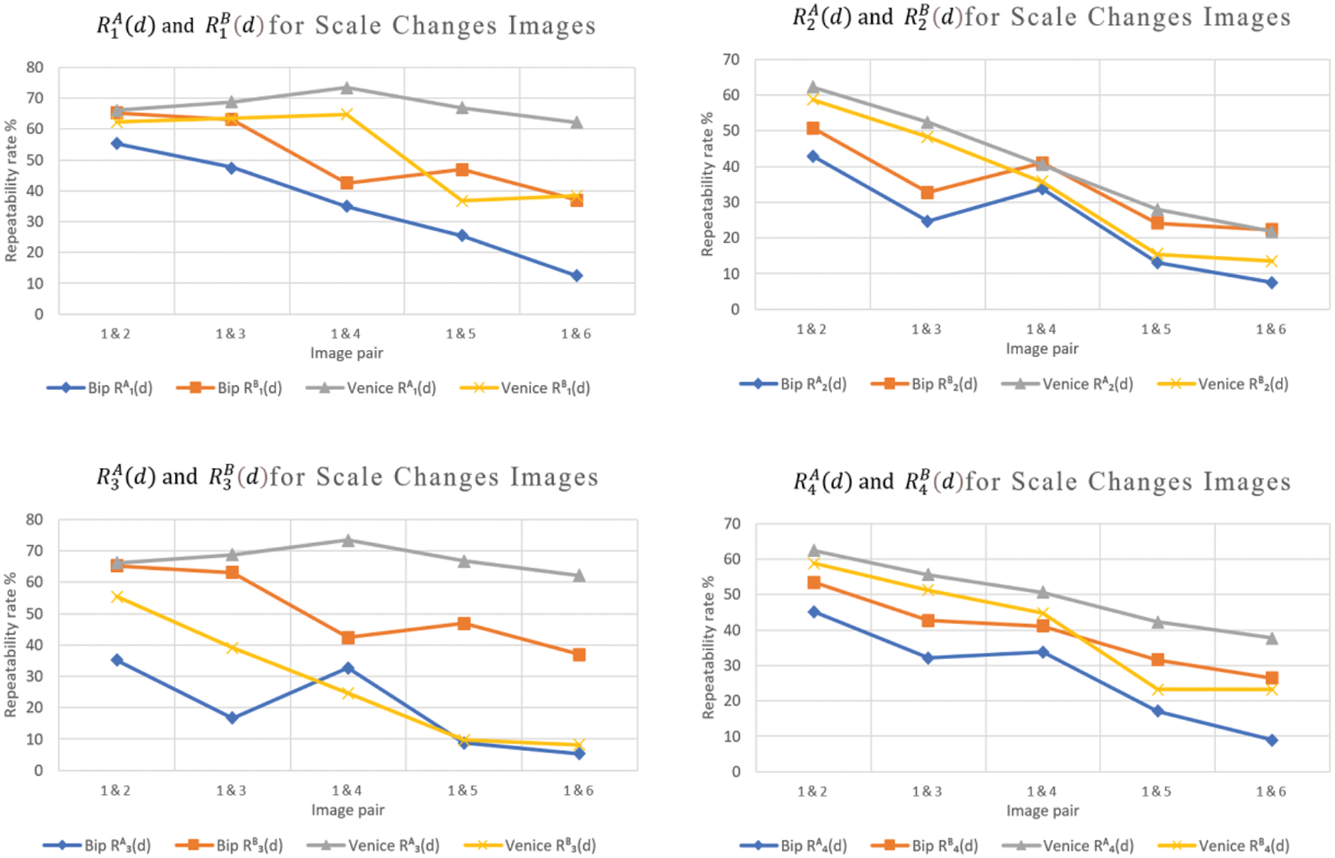
Figure 2: Examples of the repeatability rates R1X(d), R2X(d), R3X(d), and R4X(d) at d = 2 in image domains X = A and X = B for scale-change image groups. “BIP” and “Venice,” using SURF keypoint detector

3  Two-Fold Repeatability Rate Measure

The previous section’s repeatability rates are directional and image domain-dependent; this affects the measures. Consequently, all demonstrated repeatability rates are asymmetric, meaning that when the same computational process performed on one image domain is repeated on another, the results may vary. Additionally, not all the datasets’ images can be generally categorized according to their type and degree of variation [19]. Therefore, unless otherwise indicated, both directions of calculation should be considered when comparing image pairs, as long as both projections have the same d value, which represents the two-fold repeatability rate.

R(d)=<RA(d),RB(d)>(10)

A scatter diagram representation is presented to visualize and compare the two repeatability rate values concurrently.

3.1 Scatter Diagram Representation

The scatter diagram in Fig. 3 depicts the relationship between repeatability rates R1A(d) and R1B(d) that compose the two-fold measure described in Eq. (10). The computation method for the two-directional repeatability rates is similar but with different image domains (A or B). The diagram shows the change in repeatability rates for the image group “Boat” at various d values for the d-neighbor regions ranging from d = 0.5 to d = 4, with a 0.5 increment generated by the Euclidian distance from the keypoint centers to the neighbor region’s boundary. The shown curves deviate towards one axis according to the relationships between the two repeatability rates. If the two repeatability rates are equal, the plots should be on the equality line (green dashed line). The scatter diagram is helpful for groups that have variations between images, particularly scale transformations, such as the image groups shown in Figs. 3 and 4.

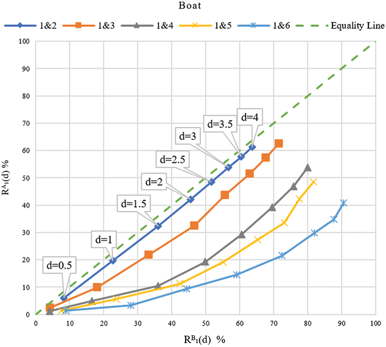
Figure 3: Scatter diagram for the two-fold repeatability rate <R1A(d),R1B(d)> at different d values for the image group “Boat.”

Fig. 4 illustrates the two-fold repeatability rate computed from the directional measures R1A(d) and R1B(d) for the “BIP” and “Venice” groups’ zoom-out and zoom-in changes. When R1A(d) > R1B(d), the curves for the zoom-out image group “BIP” are in the upper triangle, while those for the zoom-in image group “Venice” are in the lower triangle because R1A(d)< R1B(d). Consequently, the values in one of the two triangular zones in the diagram show that one repeatability rate measure is superior. However, the scatter diagram reveals plots close to the equality line for images with other geometric and photometric transformations, such as rotation changes and illumination variations. For example, Fig. 5 represents the image group “NewYork,” which has rotation variations between its images. The two repeatability rates have slight differences for such variation.

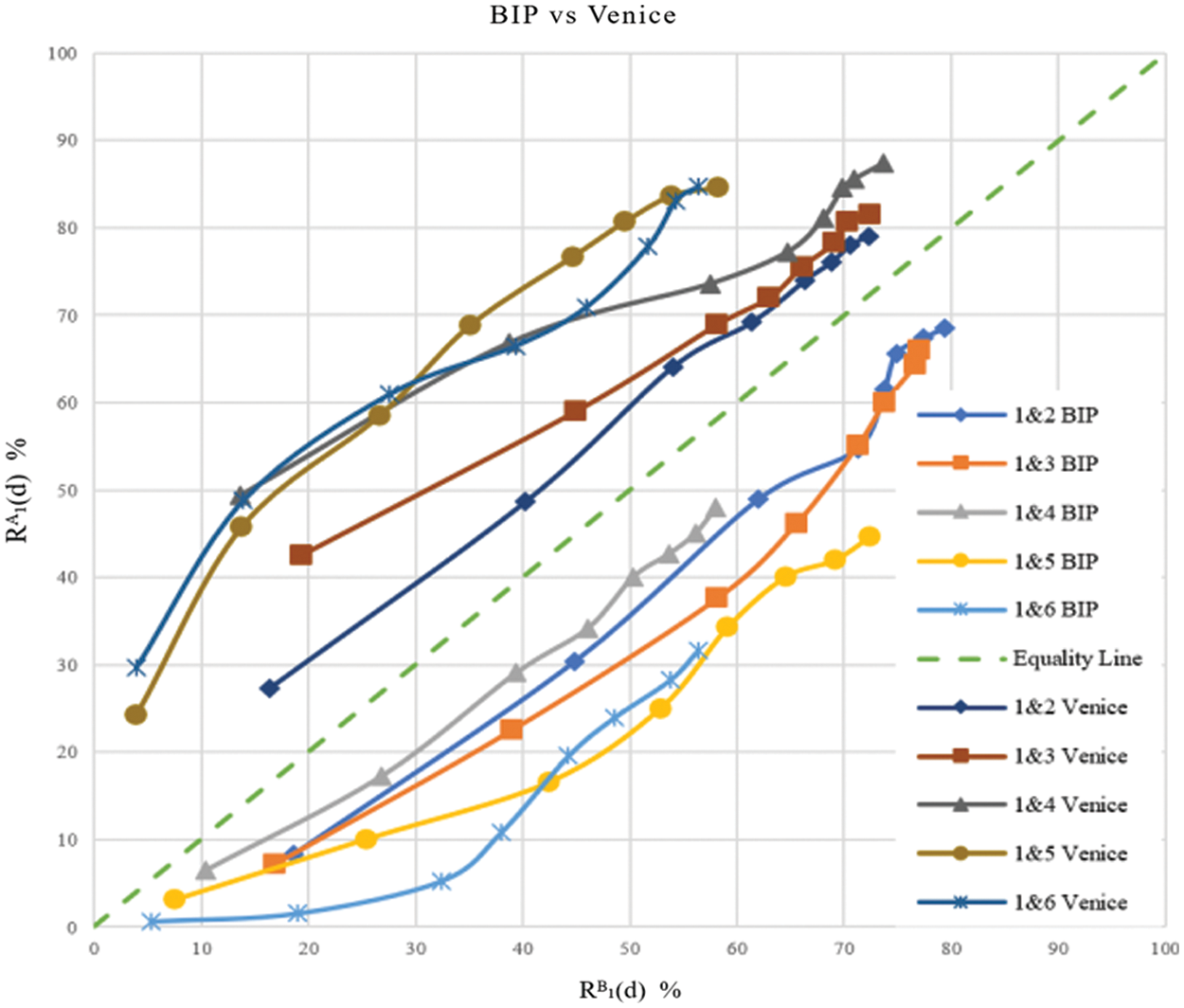
Figure 4: Scatter diagram for the two-fold repeatability rate <R1A(d),R1B(d)> computed for two scale-change image groups: “BIP” and “Venice,” with varying values of d

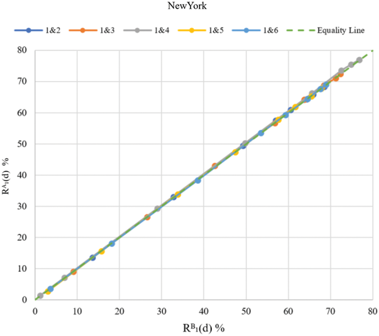
Figure 5: Scatter diagram for the two-fold repeatability rate <R1A(d),R1B(d)> computed for rotation changes image group: “NewYork,” with varying values of d

3.2 Symmetric Repeatability Rate Measurement

While the two-fold repeatability rate defined in Eq. (10) shows the values in both directions, for performance comparisons, a single value is usually required for each image pair. Thus, the repeatability rate is calculated independently for each direction. It is then combined using one of the mean calculation methods, such as arithmetic, geometric, or harmonic means. The harmonic mean is not suitable because it can divide by zero. However, the geometric mean will result in a zero-repeatability rate if one case of the directional measure equals zero. As a result, the arithmetic mean is used as a symmetric repeatability rate measurement, and it is defined as:

RiM(d)=(RiA(d)+RiB(d))2(11)

where i∈{1,2,3,4}. Tab. 1 shows the arithmetic-mean symmetric measurements for the four repeatability rate measures found in the literature and defined in Eqs. (6)–(9). The four given symmetric repeatability rates, Eqs. (11.a)–(11.d) shown in Tab. 1, have different responses to variations on the images and different keypoint detectors. The relations among the keypoints affect the calculations of the symmetric repeatability rate equations in Tab. 1. These effects are shown as different cases in Tab. 2.

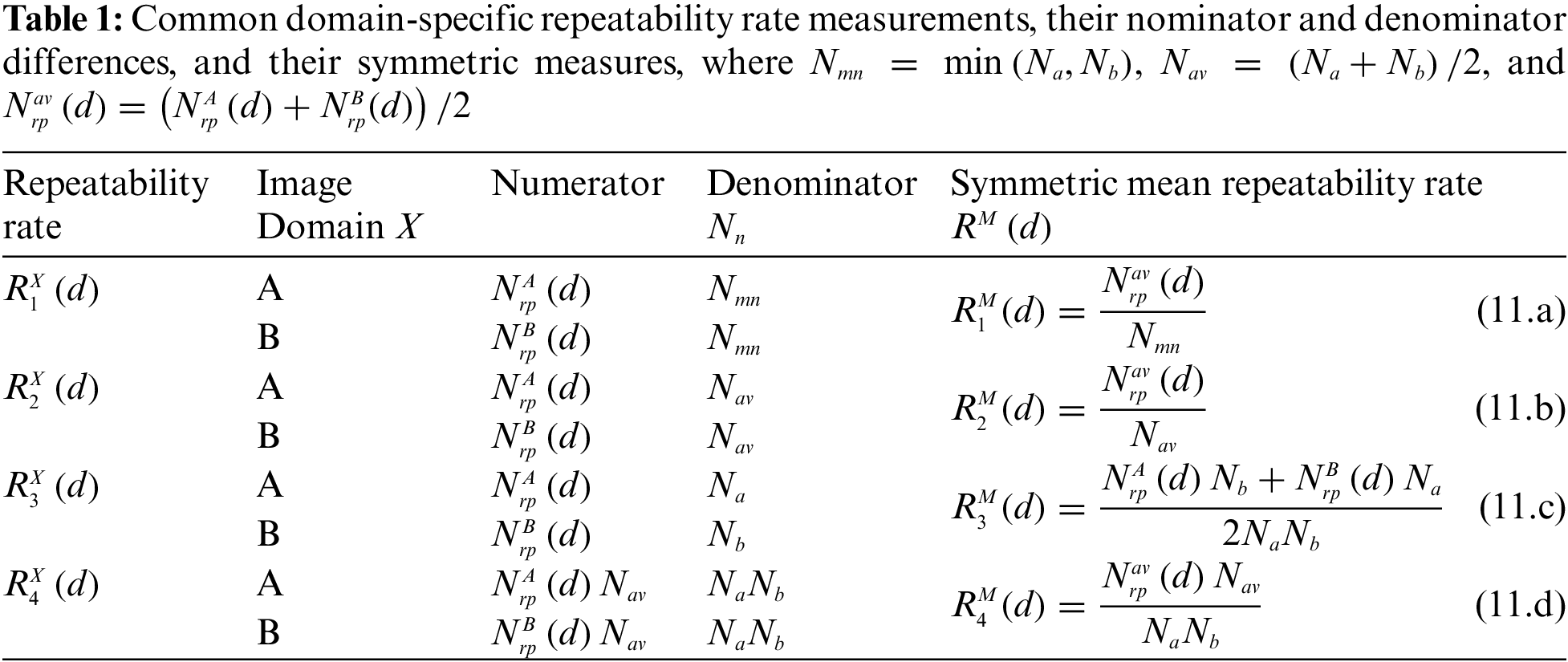
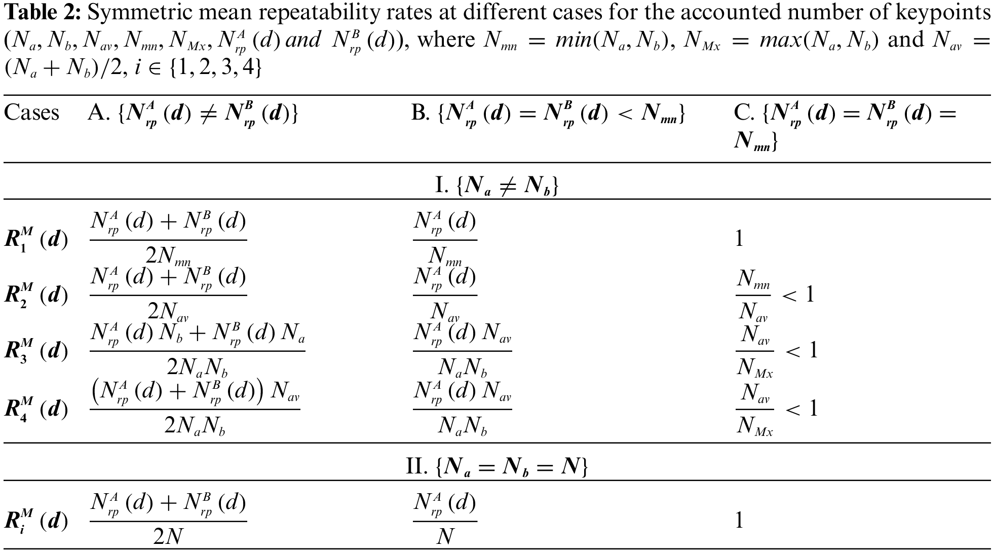
The number of surviving keypoints is assumed to be identical before and after projection to the other image domain for convenience, i.e., Na′=Na and Nb′=Nb. Furthermore, the Nmn value is significant because it represents the highest limit of keypoints count that can be repeated in the shared viewable region of the two images. Tab. 2’s findings lead to the following:

•   The number of repetitive keypoints in both domains, rather than the relationships between Na and Nb, influences the symmetrical mean repeatability rate R1M(d) because the denominator always takes the lesser of the two values. Therefore, R1M(d) has the same responses for I and II at A, B, and C cases.

•   Despite having the same numerator, R2M(d) will always be less than R1M(d) when Na≠Nb because ofNav>Nm in this case.

•   Except for the case (A-I), where the numbers of repeated keypoints and keypoints in the common region are not identical for both domains, R3M(d) and R4M(d) resemble the same equations.

•   When two conditions are satisfied (case C-II), all repeatability rates converge to one (=100%); the number of repeatable keypoints in both domains is equal to the number of visible survived keypoints in the common region of the two images. While the number of repeated keypoints in images with no scale changes (e.g., rotated images) can be similar, images meeting this criterion are uncommon unless they are nearly identical or force these numbers to be equal.

•   When {Na=Nb}, all the symmetric mean repeatability rates RiM(d) (i = 1,2,3, and 4) for the three cases A, B, and C will be similar. As a result, regardless of the relationships between repeated keypoints in the two image domains, all repeatability rate metrics in this scenario will have the same equation and thus produce the same results. In practice, case A of this situation is an uncommon for similar images.

•   Each repeatability rate may produce a different value if the common region of both images does not contain the same number of keypoints (i.e., Na≠Nb), as in the cases of I in Tab. 2.

Although some of these cases are challenging for images with noticeable changes, for example, when the repeatability rate equals 1, most of the findings in Tab. 2 are experimentally verified in the following section.

4  Experimental Results

Experiments are conducted using the symmetric measure of the two-fold repeatability rates for the four measures studied in this article. For each symmetric repeatability rate, three different keypoint detectors are tested on eight groups of images taken from two datasets ( [14] and [27]). Each group consists of 6 images and exhibits geometric or photometric changes, as shown in Fig. 6. These geometric and photometric changes, including scale (zoom-in and zoom-out), rotation, viewpoint, blur, and illumination changes, as demonstrated in Fig. 6.

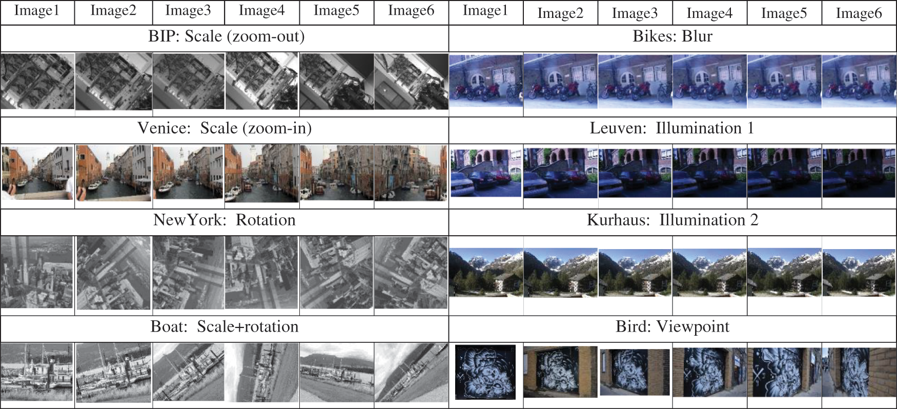
Figure 6: The eight image groups utilized in the experiments. Each group’s name and the primary variation are displayed above its images

Several keypoint evaluations have been proposed in the literature [5,28,29]. However, there is no consensus on a universally optimal detector for all possible image geometrical and photometric variations [23]. Conversely, the results in these papers indicate that the detectors tested proclaim superiority interchangeably over the others for various geometric and photometric image changes such as scale, rotation, and illumination. Consequently, the three keypoint detectors, SURF (Speeded Up Robust Features) [26], SIF (Scale Invariant Feature Transform) [30], and KAZE (which translates to ‘wind’ in Japanese) [31], were selected as examples to demonstrate the variety of responses of these detectors to the dataset presented. In addition, other keypoint detectors can be used to confirm the results. A comparison of the performance of the three mentioned keypoint detectors using the symmetric repeatability measures is in the following experiments. The experiments are conducted using built-in keypoint detectors in MATLAB 2021b software by their default parameters.

Fig. 7 shows the comparisons of the symmetric mean repeatability rates R1M(d), R2M(d), R3M(d), and R4M(d) at d = 2 using the keypoint detectors SURF, SIFT, and KAZE on the eight image groups. The results verify the derivations of Tab. 1 and Tab. 2, in which R1M(d) has the highest values because its repeatable keypoints are always divided by the minimum allocated keypoints in the common region of the tested images. R2M(d) has the lowest values because the repeatable keypoints are divided by the average keypoints in this common region. The remaining repeatability measures the range between these values as each number of repeated keypoints is individually weighted by a ratio of the survived keypoints observed in the common region. Except for the case where repeated keypoints differ in both directions, and the number of allocated keypoints in the common region is not equal, the repeatability rates R3M(d) and R4M(d) are identical in their responses. In general, the later repeatability represents the lower limit for the earlier one.

The response of the three keypoint detectors differs for the four repeatability rates due to the varying criteria for allocating keypoints. R1M(d) fails to capture the degree of transformation change, particularly for scale changes, whereas R2M(d) is more convenient in this issue. However, R2M(d) has low values even with minor image variations. The R2M(d) measure, on the other hand, attempts to maintain the trend across all keypoint detectors. While they start with the same value in most cases, R3M(d) diverges from R2M(d) toward R1M(d) in the “Boat” image group, resulting in an undesirable trend. R4M(d) has better values than R2M(d) for these images but has a lower slope than the other measures. The four rates have nearly identical values for images with rotations, such as those in the “NewYork” group, and images with modest natural illumination change, such as those in the “Kurhaus” group. In the “Leuven” group, the illumination changes uniformly on the whole image from one image to another, producing more challenges in obtaining similar keypoints in the dataset. Therefore, R3M(d) and R4M(d) have similar values that are close to R2M(d), while R1M(d) exceeds all other measures due to the difference between Na and Nb. The differences in repeatability rates are rather noticeable for image groups that include scale or blur changes. Uniform scale differences, such as those caused by zooming in and out, significantly affect directional computations over non-uniform scale differences caused by affine and higher geometric transformations.

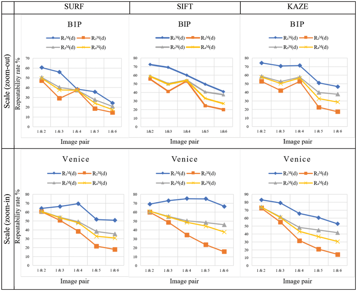
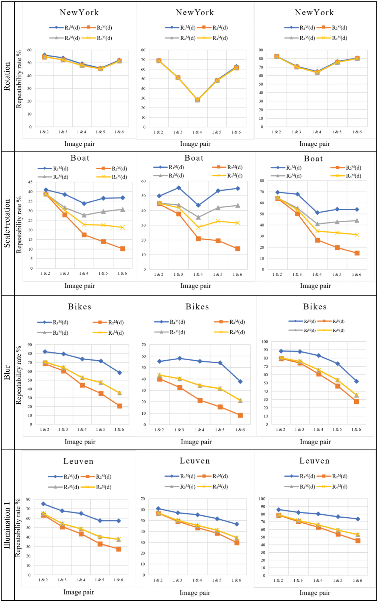
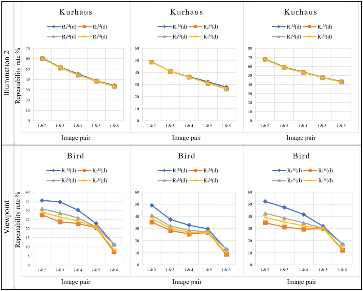
Figure 7: The symmetric mean repeatability rate measurements R1M(d), R2M(d), R3M(d), and R4M(d), as defined in Tab. 2, at d = 2, when applied to various image groups with different geometric and photometric changes

Comparing the performance of the three keypoint detectors depicted in Fig. 7 shows that the KAZE keypoint detector outperforms the other methods. Furthermore, for image groups with scale changes (e.g., scale, scale+rotation, and viewpoints), the SIFT method is superior to the SURF method, while SURF is better for blur and illumination changes.

5  Conclusions

The repeatability rate measurement is critical for evaluating and comparing the performance of keypoint detectors. However, the traditional repeatability rates demonstrated in this paper are biased with regard to the image domain in which the calculations are performed. Therefore, two-fold repeatability that represents the two values is introduced instead. The scatter plots reveal the directional repeatability rate variations that are affected by changes occurring between images. For further comparison, a symmetric measure that calculates the arithmetic mean for the two-fold repeatability rates is recommended.

When image groups with illumination, blur, and geometric variations are used to test the repeatability rates, the symmetric measurements of the four examined repeatability rates exhibit a range of responses. The repeatability rate R1M(d) produces acceptable results for images with low variation but continues a trend of disregarding the degree of transformation change. While R2M(d) resolves the issue, it returns low values for small image transformations. The other two repeatability rates have nearly identical values for small transformations. However, R3M(d) begins differing toward R1M(d) for more significant transformations. While the repeatability rate R4M(d) illustrates a good trend, it has a low slope compared to other measurements. Variation in the repeatability rates of R3M(d) and R4M(d) is limited to the values of R1M(d) and R2M(d). In general, the relationship between the four symmetric repeatability rate measurements satisfies R2M(d)≤R4M(d)≤R3M(d)≤R1M(d).

Funding Statement: The author received no specific funding for this study.

Conflicts of Interest: The author declares that he has no conflicts of interest to report regarding the present study.

References

1. T. Tuytelaars and K. Mikolajczyk, “Local invariant feature detectors: A survey,” Foundations and Trends® in Computer Graphics and Vision, vol. 3, no. 3, pp. 177–280, 2008.
2. C. Liu, J. Xu and F. Wang, “A review of keypoints’ detection and feature description in image registration,” Scientific Programming, vol. 2021, pp. 25, 2021.
3. D. DeTone, T. Malisiewicz and A. Rabinovich, “Toward geometric deep slam,” arXiv preprint arXiv:1707.07410, 2017.
4. C. Romero-González, I. García-Varea and J. Martínez-Gómez, “Shape binary patterns: An efficient local descriptor and keypoint detector for point clouds,” Multimedia Tools and Applications, vol. 81, no. 3, pp. 3577–3601, 2022.
5. A. Moghimi, T. Celik, A. Mohammadzadeh and H. Kusetogullari, “Comparison of keypoint detectors and descriptors for relative radiometric normalization of bitemporal remote sensing images,” IEEE Journal of Selected Topics in Applied Earth Observations and Remote Sensing, vol. 14, pp. 4063–4073, 2021.
6. X. Lin, C. Zhu, Q. Zhang, X. Huang and Y. Liu, “Efficient and robust corner detectors based on second-order difference of contour,” IEEE Signal Processing Letters, vol. 24, no. 9, pp. 1393–1397, 2017.
7. C. Schmid, R. Mohr and C. Bauckhage, “Evaluation of interest point detectors,” International Journal of Computer Vision, vol. 37, no. 2, pp. 151–172, 2000.
8. K. Mikolajczyk, T. Tuytelaars, C. Schmid, A. Zisserman, J. Matas et al., “A comparison of affine region detectors,” International Journal of Computer Vision, vol. 65, no. 1/2, pp. 43–72, 2005.
9. I. Rey-Otero, M. Delbracio and J. -M. Morel, “Comparing feature detectors: A bias in the repeatability criteria,” in Proc. IEEE Int. Conf. on Image Processing (ICIP), Quebec City, QC, Canada, pp. 3024–3028, 2015.
10. S. Ehsan, N. Kanwal, A. Clark and K. McDonald-Maier, “Improved repeatability measures for evaluating performance of feature detectors,” Electronics Letters, vol. 46, no. 14, pp. 998–1000, 20
11. S. Ehsan, A. Clark, A. Leonardis, N. Ur Rehman, A. Khaliq et al., “A generic framework for assessing the performance bounds of image feature detectors,” Remote Sensing, vol. 8, no. 11, pp. 928, 2016.
12. E. Rosten, R. Porter and T. Drummond, “Faster and better: A machine learning approach to corner detection,” IEEE Transactions on Pattern Analysis and Machine Intelligence, vol. 32, no. 1, pp. 105–119, 2010.
13. M. Awrangjeb and G. Lu, “Robust image corner detection based on the chord to point distance accumulation technique,” IEEE Transactions on Multimedia, vol. 10, no. 6, pp. 1059–1072, 2008.
14. [Dataset] Affine Covariant Features Datasets, Visual Geometry Group-University of Oxford, https://www.robots.ox.ac.uk/~vgg/data/affine/ (Last visited: 21 April 2022).
15. R. Haralick and L. Shapiro, Computer and Robot Vision, 1st ed., USA: Addison-Wesley Longman Publishing Co., Inc., 1992.
16. I. Rey-Otero and M. Delbracio, “Is repeatability an unbiased criterion for ranking feature detectors?,” SIAM Journal on Imaging Sciences, vol. 8, no. 4, pp. 2558–2580, 2015.
17. S. Lang, M. Luerssen and D. Powers, “Virtual ground truth, and pre-selection of 3D interest points for improved repeatability evaluation of 2D detectors,” MATEC Web of Conferences, vol. 277, pp. 2032, 2019.
18. K. Mikolajczyk and C. Schmid, “Scale & affine invariant interest point detectors,” International Journal of Computer Vision, vol. 60, no. 1, pp. 63–86, 2004.
19. K. Lenc and A. Vedaldi, “Large scale evaluation of local image feature detectors on homography datasets,” in Proc British Machine Vision Conf. BMVC, Newcastle, UK, 2018.
20. O. Kechagias-Stamatis, N. Aouf and M. Richardson, “Performance evaluation of single and cross-dimensional feature detection and description,” IET Image Processing, vol. 14, no. 10, pp. 2035–2051, 20
21. T. Mouats, N. Aouf, D. Nam and S. Vidas, “Performance evaluation of feature detectors and descriptors beyond the visible,” Journal of Intelligent. Robotics Systems, vol. 92, no. 1, pp. 33–63, 2018.
22. C. Zhang, X. Lu and T. Akashi, “Blur-countering keypoint detection via eigenvalue asymmetry,” IEEE Access, vol. 8, pp. 159077–159088, 2020.
23. S. Gauglitz, T. Höllerer and M. Turk, “Evaluation of interest point detectors and feature descriptors for visual tracking,” International Journal of Computer Vision, vol. 94, no. 3, pp. 335, 2011.
24. S. Zhang, L. Huangfu, Z. Zhang, S. Huang, P. Li et al., “Corner detection using the point-to-centroid distance technique,” IET Image Processing, vol. 14, no. 14, pp. 3385–3392, 2020.
25. S. Zhang, B. Li, M. Chen, Y. Sang and M. Huang, “Feature detection using relative distance and multi-scale technique,” Alexandria Engineering Journal, vol. 61, no. 11, pp. 8585–8593, 2022.
26. H. Bay, T. Tuytelaars and L. Van Gool, “Surf: Speeded up robust features,” in European Conf. On Computer Vision, Graz, Austria, Springer, pp. 404–417, 2006.
27. V. Balntas, K. Lenc, A. Vedaldi and Kn Mikolajczyk, “HPatches: A benchmark and evaluation of handcrafted and learned local descriptors,” CVPR, 2017. [Online]. Available: http://icvl.ee.ic.ac.uk/vbalnt/hpatches/hpatches-sequences-release.tar.gz.
28. Y. Ou, Z. Cai, J. Lu, J. Dong and Y. Ling, “Evaluation of image feature detection and matching algorithms,” in 5th Int. Conf. on Computer and Communication Systems (ICCCS), Shanghai, China, pp. 220–224, 2020.
29. S. Tareen and Z. Saleem, “A comparative analysis of SIFT, SURF, KAZE, AKAZE, ORB, and BRISK,” in Proc Int. Conf. on Computing, Mathematics and Engineering Technologies (iCoMET’18), Washington, DC, IEEE, pp. 1–10, 2018.
30. D. G. Lowe, “Distinctive image features from scale invariant keypoints,” International Journal of Computer Vision, vol. 60, no. 2, pp. 91–110, 2004.
31. P. F. Alcantarilla, A. Bartoli and A. J. Davison, “Kaze features,” in European Conf. on Computer Vision, Florence, Italy, Springer, pp. 214–227, 2012.

This work is licensed under a Creative Commons Attribution 4.0 International License, which permits unrestricted use, distribution, and reproduction in any medium, provided the original work is properly cited.