| Computers, Materials & Continua DOI:10.32604/cmc.2022.031734 | |
| Article |
An Effective Classifier Model for Imbalanced Network Attack Data
Department of Information System Engineering, Mugla Sıtkı Koçman University, Mugla, 48000, Turkey
*Corresponding Author: Gürcan Çetin. Email: gcetin@mu.edu.tr
Received: 25 April 2022; Accepted: 07 June 2022
Abstract: Recently, machine learning algorithms have been used in the detection and classification of network attacks. The performance of the algorithms has been evaluated by using benchmark network intrusion datasets such as DARPA98, KDD’99, NSL-KDD, UNSW-NB15, and Caida DDoS. However, these datasets have two major challenges: imbalanced data and high-dimensional data. Obtaining high accuracy for all attack types in the dataset allows for high accuracy in imbalanced datasets. On the other hand, having a large number of features increases the runtime load on the algorithms. A novel model is proposed in this paper to overcome these two concerns. The number of features in the model, which has been tested at CICIDS2017, is initially optimized by using genetic algorithms. This optimum feature set has been used to classify network attacks with six well-known classifiers according to high f1-score and g-mean value in minimum time. Afterwards, a multi-layer perceptron based ensemble learning approach has been applied to improve the models’ overall performance. The experimental results show that the suggested model is acceptable for feature selection as well as classifying network attacks in an imbalanced dataset, with a high f1-score (0.91) and g-mean (0.99) value. Furthermore, it has outperformed base classifier models and voting procedures.
Keywords: Ensemble methods; feature selection; genetic algorithm; multilayer perceptron; network attacks; imbalanced data
The most important instrument offered for fulfilling security criteria in the area of cybersecurity is an Intrusion Detection System (IDS). It utilizes two types of the detection strategies: signature-based detection and anomaly detection. Signature-based IDSs aim to match events and traffic to pre-defined attack patterns using a database of the security attack signatures [1]. On the other hand, anomaly detection examines the data to see if anything unusual is occurring. Both techniques suffer from poor detection rates and high false alarm rates [2]. The performance of IDSs can be enhanced by the use of the machine learning algorithms [3]. The goal of the machine learning (ML) algorithms is to discriminate between normal network traffic and other types of intrusions. Many studies [4–8] have been conducted on which ML algorithms are suitable, and which parameter values should be selected. The using of the benchmark network attack datasets such as DARPA, KDD-Cup’99, NSL-KDD, Kyoto2006+, CAIDA-2007 and CICIDS2017 are the most popular approach for testing the performance of the ML algorithms [9].
Network attack datasets face two major challenges: imbalanced data and high-dimensional data. The number of attacks in the CICIDS2017 is an example of the problem of class imbalance. While there are 2,830,743 entries in this attack dataset, only 11 are related to “hearthbleed” and 21 are related to “web attack SQL injection” attacks. However, the ability of a robust IDS to categorize all attack types will increase its efficiency. To improve the performance of the classification, there are algorithm-based, data-based (undersampling and oversampling) or hybrid techniques [10]. When the literature studies are examined, it is seen that many studies make performance evaluations according to the macro averages of the classical methods such as accuracy and precision. Nevertheless, traditional metrics for imbalanced data sets are not useful for measuring the performance of these algorithms. This is due to their high bias towards the majority class [11].
Another difficulty with network attack datasets is the number of features. While not all of these features contribute equally to explaining the remaining information in the data, overfitting occurs affecting the accuracy of the ML model negatively. Because of this dimensionality, the training and testing phases of ML may necessitate more memory requirements and computational cost [12,13]. The KDD-Cup’99 and NSL-KDD datasets, for example, include 42 features, the Kyoto 2006+ dataset has 48 features and the CICIDS2017 dataset has 79 features [9]. The high-dimensional data spaces degrade the performance of the ML-based IDSs. As a result, it is critical to choose an appropriate feature selection (FS) strategy that may eliminate those features. There are three approaches to feature selection: statistical (Chi-Square), entropy-based (Information Gain, Symmetric Uncertainty), and sample-based (ReliefF). Nonetheless, the strategies of these FS algorithms often negatively affect the success of the subsequent classifications. In other words, a selected feature subset that works successfully for one class may reduce the performance of the determining another class [14].
In this paper, a model is proposed to address these two problems using the CICIDS2017 dataset. The first challenge is to select features that can be used to classify each type of attack and normal traffic data equally. A genetic algorithm-based feature selection (GAbFS) approach has been utilized to address this challenge. In minimizing the number of features with a genetic algorithm (GA), the average highest f1-score values (macro average) of the base classification methods have been utilized as the objective function. Removing irrelevant features from the data decreases False Positives (FPs) and False Negatives (FNs) while improving the classifier’s learning rate, detection accuracy [13], and f1-score value. The performance of the GAbFS has been compared with Recursive Feature Elimination (RFE), Random Forest (RF) and Linear models.
The second challenge is the high-performance classification of all attack types with reduced features on the imbalanced CICIDS2017 dataset. In this study, a multilayer perceptron (MLP) based ensemble method has been developed to overcome this difficulty and increase the overall performance. Multiple base-classifiers are constructed using classic ensemble techniques in order to make predictions about unknown data by voting [15]. However, in the proposed MLP-based ensemble method uses the estimations of the selected base classifiers as input to the MLP model to predict the attack type. At the end of the study, the overall performance of the proposed system has been assessed using the f1-score, and g-mean value criteria, and compared with traditional voting methods.
The study is divided into the following sections: Section 2 discusses related efforts on the network attack classification with feature selection and ensemble learning. The concepts of the GA, MLP, classification algorithms, and ensemble methods are explained in Section 3, while the CICIDS2017 dataset is explained in Section 4. The general model of the proposed method is detailed in Section 5. Section 6 includes the models’ assessment criteria, the study’s experimental results, the findings, and discussions. Section 7 brings the research to a close.
Many studies have been offered in order to find effective solutions to the imbalanced and high-dimensional data problems of the network attack datasets. The classification performance of the offered approaches varies according to the selected ensemble algorithms and the number of features.
Kurniabudi et al. [16], in their study on the CICIDS2017 dataset, used Information Gain, ranking and grouping the features methods for FS. The dataset with decreased features has been subjected to RF, Bayes Net (BN), Random Tree (RT), and Naive Bayes (NB) analysis. The test findings revealed that the number of features chosen by Information Gain has a substantial impact on the performance and execution time. Khsirsagar et al. [17] has been used the FS approach to categorize “DoS attacks” in the CICIDS2017 dataset. A FS approach based on a combination of the Information Gain, Correlation, and ReliefF algorithms has been proposed. The system first generates subsets of the features for each classifier based on the average weight, and then employs the Subset Combination Strategy (SCS). The suggested FS strategy decreased the number of features in the CICIDS2017 to 24 and in KDD-Cup’99 to 12. The accuracy of the system for “DoS attacks” is 99.95%.
Chohra et al. [18] presented an optimization strategy for solving the FS challenge that incorporates swarm intelligence and ensemble approaches. The features picked during the optimization phase, and then the technique used automated encoders in each dataset to develop a deep learning-based anomaly detection model. With an f1-score of 0.92 in the NSL-KDD dataset, 0.929 f1-score in the UNSW-NB15 dataset, and f1-score of 0.973 in the IoT-Zeek dataset, the model outperformed state-of-the-art ML algorithms.
Özgür et al. [19] proposed a model that uses GA to accomplish FS and weight selection for classifier fusion. The NSL-KDD has been used as the dataset. In addition, classifier selections have been made for fusion from base classifier algorithms, with at least 2 and at most 8. The 41 features have been decreased to 21. The use of the GAbFS decreased training time by 30% to 34% and testing time by 23% to 25%. The weighted f1-score has been obtained 0.908 after applying classification fusion. In the most successful classifier fusions, AdaBoost, Decision Tree (DT), Logistic Regression (LR), and K-Nearest Neighbor (KNN) base classifiers have been employed. On the other hand, as the number of the fusion classifiers increased, the success values declined.
Moukafih et al. [20] introduced the neural network-based voting system for IDSs. The approach created feed-forward neural networks as weak learners. And then, an ensemble module combines the predictions of the weak learners to produce a majority vote. As a result of the tests performed on the NSL-KDD, 0.89 accuracy and 0.9 f1-score values have been obtained.
The Genetic Algorithm (GA) is a stochastic optimization algorithm based on natural selection theory. In GA-based problem solutions, gene structure is encoded in a binary system generally. These genes are also representatives of the population. By modifying the genes in the population across generations, searches are undertaken in different parts of the solution space [19].
According to the GA, an initial population is primarily produced based on the possible solution space. The numerical model of the problem is utilized to calculate the objective function and individual fitness. The selection, crossover, and mutation steps are then repeated for each individual in the population. The selection stage is the process of selecting good individuals from the existing population. Thus, better individuals are used to produce the next generation. The roulette wheel and the tournament are the most prevalent methods of the selection [21]. Crossover and mutation genetic operators, on the other hand, are the most significant components of the GAs. The crossover produces a new individual by exchanging some genes between matched parents, whereas the mutation produces a new individual by randomly altering the value of a gene on a chromosome. The mutation operator is critical for preserving population variety and increasing the probability of the reaching global optimization [22]. However, thanks to elitism, a set of candidate individuals is preserved at each iteration, ensuring that some of the most successful genes are passed on to the next generation unchanged [19]. Following these steps, a new population arises, and objective functions for this population are determined. This iterative procedure is repeated until the stopping criterion is met.
Deep learning has emerged as a popular research topic in the field of artificial intelligence in recent years [23]. The MLP, one of the deep learning methods, is a supervised learning neural network structure. This feed-forward network architecture uses pre-labeled training samples to map unknown data to a label. An MLP network is made up of neurons and layers that process and categorize data according to the network’s demands [24]. Each neuron in one layer has a weighted connection to each node in the following layer [25].
As indicated in Fig. 1, an MLP contains three primary levels: an input layer, an output layer, and one or more hidden layers. The first layer of the MLP model is the input layer, which is indicated by X = x1, x2,…, xn. Its role is to accept the input data. The output layer of MLP is represented by the expression Y = y1, y2,…, yn. Each class label in the training dataset is represented by the nodes. The hidden layer is one of MLP’s most critical layers. The hidden layer’s activation functions determine whether or not a neuron is activated. It accomplishes this by doing computations based on data and a learning algorithm [26]. The equation for a node in a hidden layer is given in Eq. (1).
where; h1j is the jth node in the h1 hidden layer. f(.) is a nonlinear activation function that can be any of the following: linear, sigmoid, tanh, or ReLU. The bm is the bias, and wij represents the weight associated with the xth input entering the jth node of the hidden layer h1 [25]. At the feed-forward level, weight connections are given random values at first. However, throughout the gradient descent process, the error between the predicted and actual labels is calculated, and the weights and bias values are updated by iterative reduction at the back-forward level [24].
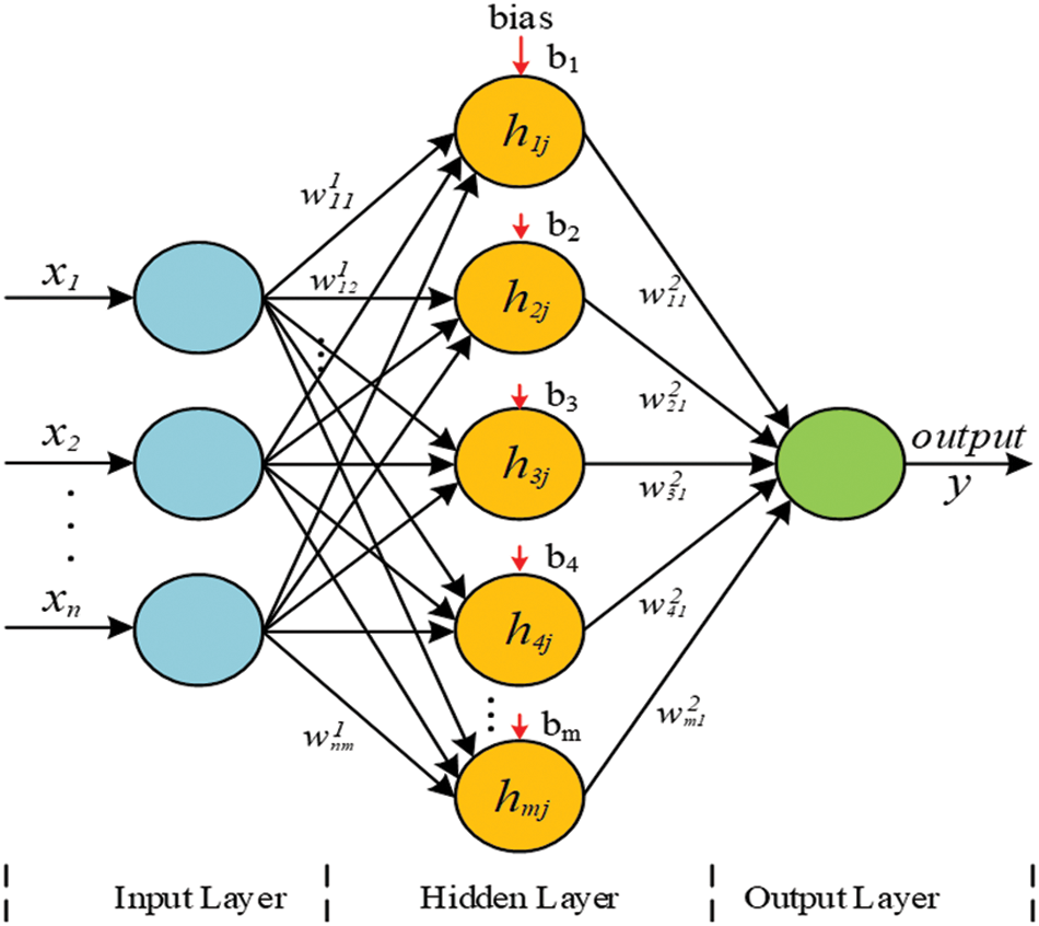
Figure 1: Multi-layer perceptron topology
Ensemble learning is a methodology that combines low-performance classifiers to produce a high-performance classifier [27]. Instead of constructing a single complex and powerful classifier, the basic principle of ensemble learning is to combine several weak and simple classifiers to enhance the accuracy of the prediction rate. Fig. 2 depicts a common ensemble learning framework. With reference to Fig. 2, the dataset is separated into two parts: test and training. A stronger model was created by applying N weak models to both datasets.
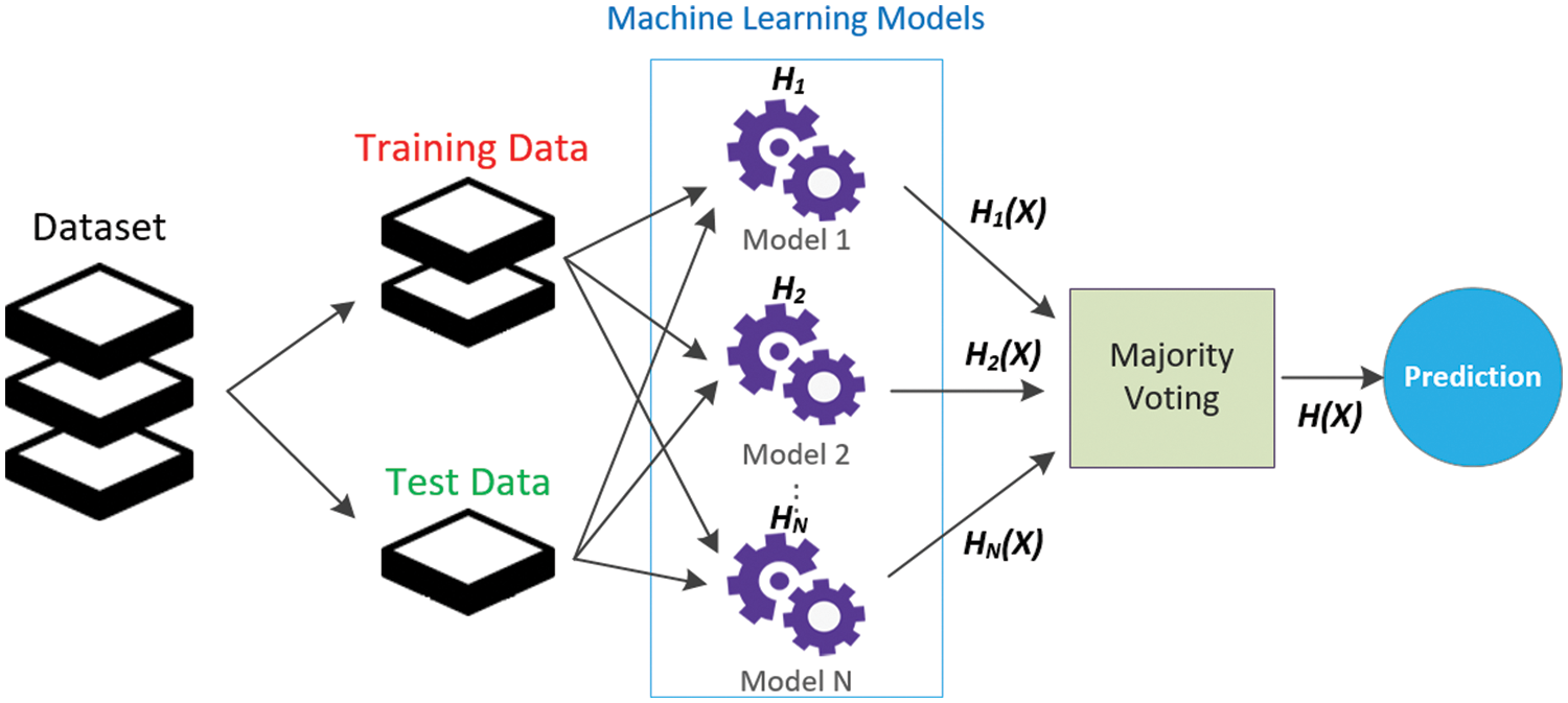
Figure 2: The general structure of the ensemble learning
According to Fig. 2, it is assumed that the nth weak classifier is indicated by Hn : X → {1, +1}, for n = 1,…,N, and (x ɛ X) is the classification input. In addition, the outputs of the N classifiers (H1(x), H2(x) ,…, HN(x)) can be combined into a single ensemble classifier (H(x)) in a variety of ways. Based on Eq. (2), a single strong classifier can be calculated by giving a weighted combination of the weak classifiers, where (w1, w2, …, wN) indicates a collection of the classifier weights. At each epoch of the algorithm, each instance from the training dataset gets a weight based on the degree of accuracy of the previous weak classifiers, and therefore the algorithm attaches importance to the misclassified examples [28].
The main purpose of the classification process is to predict which class the new input data belongs to in a dataset with many different data categories [29]. If a classification process generates one of two outputs for an input data, it is referred as “binary classification”. On the other hand, if a classification task is carried out for more than two classes, it is called “multi-class classification”. There are a wide variety of the classification algorithms, and the basic ones have been used in this study. If these are summarized; The LR is frequently used for binary classification tasks. If the learning method employs one-vs.-rest, it can also be utilized for multi-class classification tasks [12]. The NB classifier is based on the Bayes theorem for classification tasks. It learns probability information from current features and applies it to unknown features. The NB algorithm deals with nonlinear parameters. As a result, it is robust to outliers. The KNN is a supervised ML technique that predicts each class based on the target’s feature similarity. To determine similarity between data points, it employs the Euclidean distance, Manhattan distance, chi-square, and cosine similarity methods. The KNN classifier performs better with fewer input variables and the same data size [30]. A Support Vector Machine (SVM) is used as a classifier to aid in the determination of suitable decision boundaries or hyperplanes for performing multiple tasks. Depending on the type of used kernel (linear, polynomial, or rbf), linearly separable and non-linearly separable issues can be addressed [31]. The DT is a method for creating or improving classifying models in the shape of a tree [32]. Overfitting is one of DT’s most significant matters. To overcome this problem, the RF model randomly selects and trains alternative subsets from both the data set and the feature set.
The overall performance of the proposed system has been evaluated using the accuracy, precision, f1-score, and g-mean metrics. All of these metrics are based on the number of true positive (TP), true negative (TN), false positive (FP) and false negative (FN) predictions. According to the formulas given in Eqs. (3)–(8). The precision indicates how many positively predicted data are actually positive. A classifier with high precision is considered good. On the other hand, the accuracy of positive predictions is measured by recall, whereas the accuracy of negative predictions is measured by specificity.
The harmonic mean of a classifier’s precision and recall is combined into a single statistic by the f1-score. One of the most important reasons to use it, is to avoid selecting the wrong model in imbalanced data sets. G-mean measures the balance between classification performances in the majority and minority classes. Even with enough TN predictions, a low g-mean score suggests that the model’s TP performance is inadequate. Balanced accuracy score (BAS) should be used to measure accuracy in the event of extremely imbalanced data.
The Canadian Cyber Security Institute’s CICIDS2017 dataset has been used in the research. Sharafaldin et al. [4], in order to produce a comprehensive content in the dataset, they employed two alternative network; the attack and victim networks. It based on HTTP, HTTPS, FTP, SSH, and e-mail protocols [6,8]. These statistics were taken during a 5-day period between 09:00–17:00 on weekdays. The network traffic feature information collected via the CICFlowMeter program has been reduced to 78. The features in CICIDS2017 dataset are listed in Tab. 1.

After all data was labeled, the dataset was reduced to 14 attack categories and normal packet data [33]. Tab. 2 shows the types of attacks carried out in the CICID2017 dataset, as well as the ratio of these attacks in the overall dataset. According to Tab. 2, the dataset generated a total of 6 attack profiles from the list of the frequent attack types. DoS, PortScan, Bot, Brute-Force, Web Attack, and Infiltration are examples of such threats. For example, with 158,930 attacks, PortScan attacks represent 5.61 percent of the overall dataset, whereas Web Attacks account for 0.077 percent. Furthermore, at 0.00127 percent, the Infiltration attack has the lowest value.

This section proposes a new model for high-performance classification of the attack types in the imbalanced network attack datasets. This approach consists of three fundamental and successive phases, as shown in Fig. 3. First, data preprocessing steps on the CICIDS2017 dataset are performed, then features and strong classification algorithms are selected with genetic algorithm. Finally, overall performance is improved by combining selected features and classification algorithms in an MLP-based ensemble method.
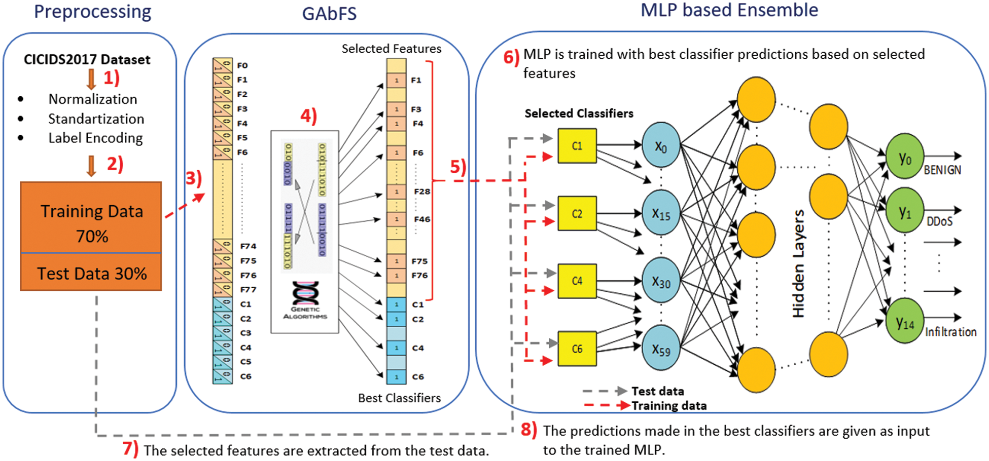
Figure 3: The diagram of the proposed model
The following are the data preprocessing methods performed for the CICIDS2017 dataset in the study: (1) 1358 data with NAN and NULL values have been extracted from the data set. (2) The Categorical data in the ‘label’ feature were digitized in the binary format by using One Hot Encoder. (3) The cleaned and corrected data has been subjected to Z-Score scaling. (4) The dataset has been split into two parts: 70% training and 30% testing. At this stage, the distribution of attack types and BENIGN data has been ensured to be equal in the both datasets. For example, 70% of the 5796 slowloris attack data has been moved to the training set and 30% to the test set.
5.2 Feature Selection Using Genetic Algorithms
A genetic algorithm-based feature selection (GAbFS) strategy is used in this study to select features. Furthermore, another goal of the suggested technique is to choose the most powerful classifiers from among the fundamental classification algorithms. Fig. 4 depicts the suggested model’s binary chromosomal sequence. The chromosomal organization is divided into two sections: feature genes and classifier genes.
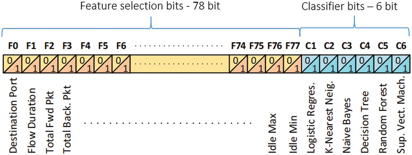
Figure 4: Binary chromosomal sequence of the GAbFS
A binary gene structure has been encoded for 78 features in the CICIDS2017 dataset. If a bit has a value of 0, the feature indicated that gene is not selected; if it has a value of 1, the feature is selected. For example, considering the feature ID values given in Tab. 1, the “destination port” and “total backward packets” features will be selected for a chromosome starting with “10010…”. On the other hand, the features “flow duration”, “total fwd packets” and “total length of fwd packets” will not be used in the calculation of the objective function.
Studies have shown that suitable algorithms vary depending on the datasets, and the performance of these algorithms is highly tied to the characteristics of the datasets [35]. For this purpose, a 6-bit classifier gene is placed at the end of the feature genes. The 6 bits, each representing a method, decide whether base classifiers LR, NB, KNN, DT, RF, and SVM will be used in the performance calculation. So, the relationship between each selected feature and the candidate algorithms’ performance has been studied. The hyper parameter values of the used classifiers are given in Tab. 3.

In the minimizing the number of features by the GA, the mean highest f1-score values (macro average) of the selected basic classification methods have been used as the objective function. The classifiers are trained on the training dataset with the features selected by the GA. The final success of the model is tested on test data that has never been seen by the GA. The GA parameters and values are given in Tab. 4.

In the following stage, the predicted values derived by employing the GA-selected features and the four most powerful classifiers are input into the MLP network in the binary format. The purpose is to train the MLP network utilizing predicted data labeled by the defined classifiers as well as the actual values at the output. Each classifier’s prediction data is a 15-bit array that represents 15 separate cases (benign or attack types). As a result, the MLP network has 4 × 15 = 60 inputs. On the other hand, the MLP includes 15 outputs, which indicate BENING or attack kinds, and there are 3 hidden layers. The number of the neurons in the hidden layers is 105, 55, and 28, respectively. The ReLU as the activation function for hidden layers. The adam algorithm as an optimizer and learning rate = 0.001 has been chosen.
The overall performance of the suggested model has been assessed with test data at the end of the study. The selected features have been extracted from the test data first, and then the strong classifiers produce new prediction values. The trained MLP network receives these prediction values as inputs, and the unknown inputs are mapped to a label with high performance.
The research has been carried out in Python, with 8 GB RAM and an Intel-Core i7 1.80 GHz CPU. The multi-class performance macro-averaged metrics have been used to evaluate the performance of the classifiers. Accordingly, the findings of the study have been evaluated from two perspectives.
6.1 Evaluation of the GA Based Feature and Classifier Selection
The GAbFS method aims to get the best classification performance by using the least number of features in the CICIDS2017 dataset. Tab. 5 lists the 23 features that the GAbFS algorithm determined to be the most optimal after 50 iterations.

The GAbFS approach has been also employed to choose the top 4 base classifiers based on the selected features. Tab. 6 displays the results depending on the selected features. RF is the most effective classifier, with 0.88 f1-score, 0.819 g-mean, and 0.878 BAS values. A BAS value close to 1.0 indicates a highly accurate prediction for each class. On the other hand, LR has the weakest classification performance, with 0.35 f1-score, 0.001 g-mean, and 0.333 BAS. A g-mean value of 0.001 indicates that the ratio of TP and TN for LR is quite low. As a result, RF, DT, and KNN classifiers have good g-mean, f1-score, and BAS value. SVM has been chosen as a fourth classifier because it showed the highest performance after the three classifiers.

The GAbFS method has been compared with the RFE, RF, Ridge, and Lasso Regression algorithms that rank the features in order of importance. The rank values for the first 23 features sorted by Mean values, are given in Tab. 7. Each model calculated the impact of the features for a range of 0.0 to 1.0 (normalized with min-max). While Average Packet Size in the RFE technique has the greatest rank value, Subflow Fwd Bytes in Ridge, Max Packet Length in Lasso, and Bwd Packet Length Max in RF have the highest rank value. For this reason, the study has been also compared by calculating the Mean rank value.

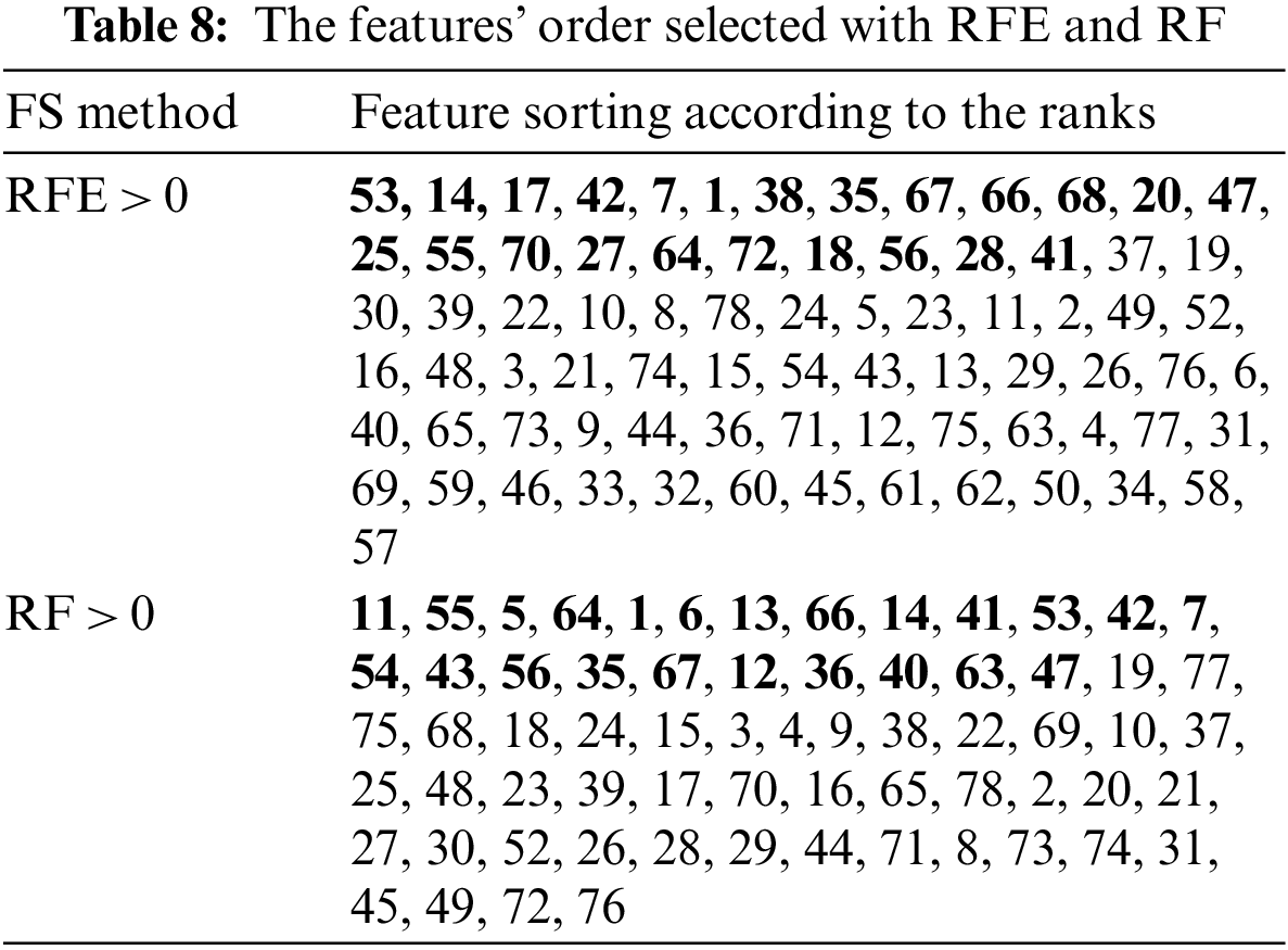
The RFE and RF are other feature selection techniques compared in the study. Tab. 8 lists the features with their rank. This table excludes features having a rank of zero. The classification performances of the features chosen by RFE, RF, and Mean have been compared. Tab. 8 shows 23 selected features highlighted in bold.
The f1-score and g-mean criteria are used to evaluate classifier performances based on the features identified by RFE, RF, and Mean in Tab. 9. When the RFE approach has been compared to the GAbFS, the performance of the SVM and KNN algorithms is worse than selected 23 features. The value of g-mean = 0.682 for KNN clearly demonstrates this. As a result, in the KNN algorithm calculations, the TP and TN ratios fell. The same is true for Mean. On the other hand, according to the features selected with RF, the performance ratios remained at the lowest values. This is particularly obvious in the small number of attack packages in the dataset. The DT classifier, for example, has got an f1-score of 0.04 for a Web XSS attack, 0.20 for SQL Injection, and 0.53 for Bot. This indicates that the features used to classify these attack types have reduced performance.

The extent to which the selected features impact the execution time of the algorithms and the peak size of all traced memory values has been investigated at the end of the GAbFS procedure. Figs. 5a and 5b shows the results from the RF and DT classifier models having the highest performance values. The data type for all selected features is float64. According to Fig. 5a, the max memory size for 78 features in the DT method was 529.42 MB, but for 23 features this value has been reduced to 198.2 MB, resulting in a 62.5% performance increase. Similarly, the highest memory usage in the RF algorithm was 1237.23 MB, which has been reduced to 948.45 MB using the GAbFS method.
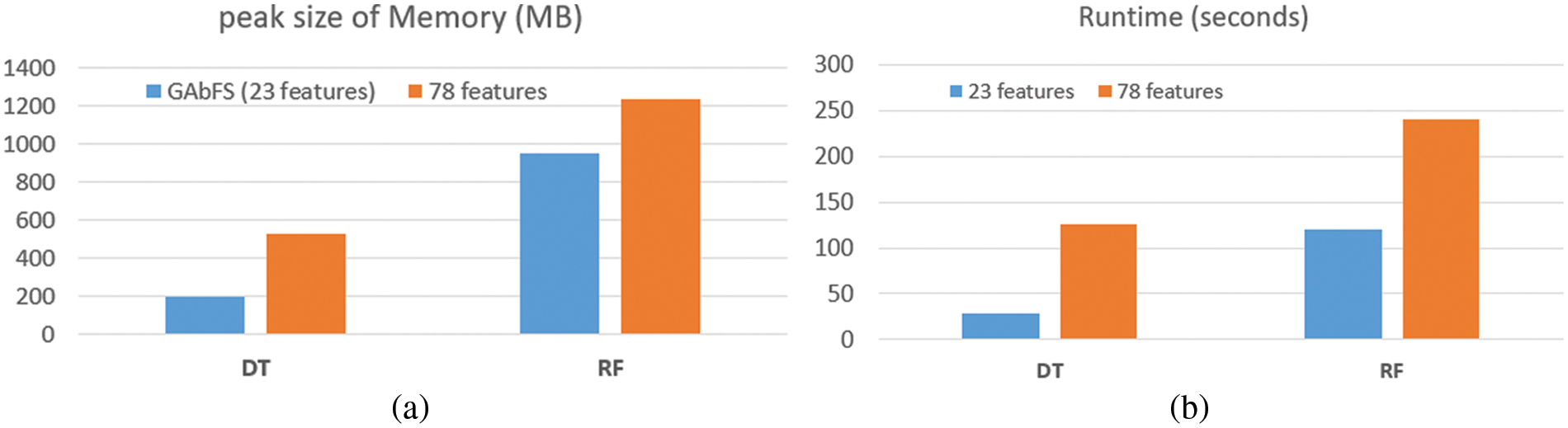
Figure 5: a) Max memory consumption values b) Runtime values of the DT and RF algorithms
Fig. 5b depicts the runtime statistics. According to the DT algorithm, the working speed has risen nearly 4.4 times, which is a significant increase. In the RF algorithm, this increase rate remained 2 times. When the algorithms’ performance is measured in terms of memory consumption and runtime, it is clear that feature reduction considerably improves their performance.
6.2 Evaluation of the MLP Based Ensemble
The estimation values of the DT, RF, KNN, and SVM classifiers, chosen by using the GAbFS approach based on the highest f1-score, have been given into the MLP model as input. Fig. 6 shows the loss curve obtained during the MLP model’s training and testing. The training and test loss curves showed that the model fitted well to the training and test data. The MLP-based ensemble method has increased the overall performance of the system to 0.91 f1-score.
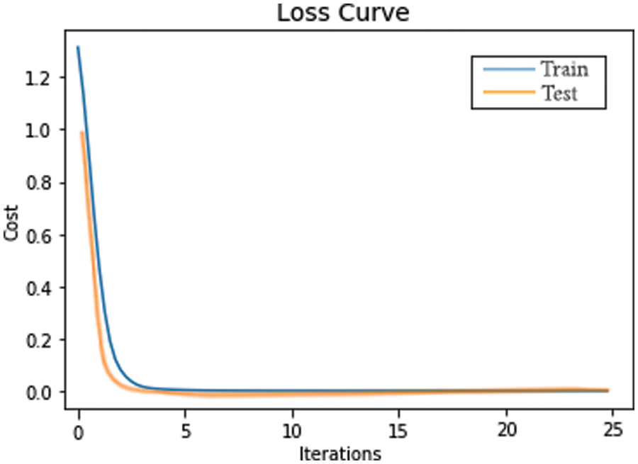
Figure 6: Train and test loss curves in the MLP
The performance results of the MLP-based ensemble method in classifying network attacks are given in Tab. 10. Based on the model’s overall evaluation, the MLP-based ensemble technique acquired a precision value of 0.93 and a recall value of 0.89. It can be said that the values estimated as positive are generally positive. The model, on the other hand, has an f1-score of 0.91 and a g-mean of 0.99. According to these results, the suggested model is a robust classification model. When the classification performances are analyzed according to the attack classes, it is seen that the performance is low for the 13 and 14 attack classes. The comparison matrix in Fig. 7 shows the reasons behind this condition in detail.

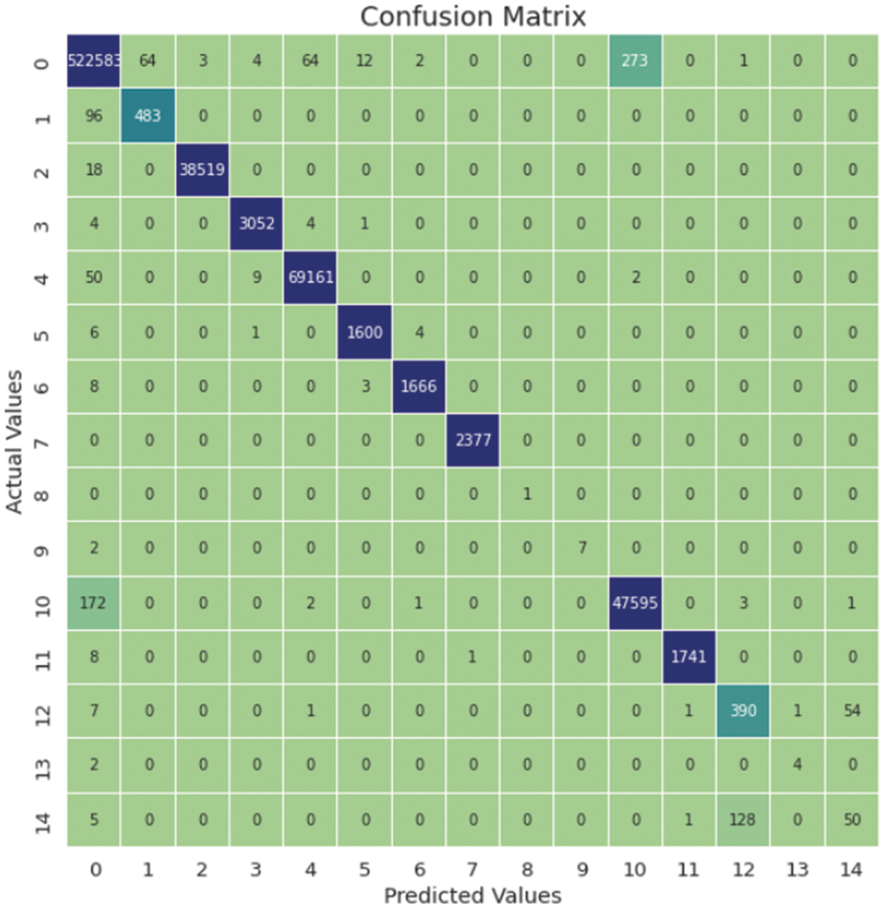
Figure 7: Confusion matrix of the MLP-based ensemble results
According to the confusion matrix in Fig. 7, the Web Attack XSS number 14 has been mostly predicted as the Brute Force number 12. In this case, 128 of the 184 Web Attack XSS data included in the test data have been mislabeled as Brute Force. Only 4 out of the 6 SQL Injection attacks were correctly classified in the 13th attack. BENIGN is labeled for 2 data.
The collected findings have been compared to the values of the hard, soft and weighted ensemble models; the results are summarized in Tab. 11. The weighted ensemble technique has been performed the best, with 0.89 f1-score and 0.85 g-mean values, while the hard voting method has been performed the worst, with 0.85 f1-score and 0.69 g-mean values. The proposed MLP-based ensemble technique outperformed all of these methods.

The research concludes with a qualitative discussion of the applicability of the proposed models, which compares the proposed model to related studies already available in the literature. It should be noted, however, that only research based on the CICID2017 dataset is discussed here, with a primary focus on feature selection and ensemble techniques. Tab. 12 summarizes the literature, with a focus on the performance results of the feature selection methodologies.

The authors in [17] developed a model based on the Information Gain Ratio, Correlation, and ReliefF algorithm. The Subset Combination strategy was used in the model to produce feature subsets for each classifier based on the average weight. The study focused solely on features for detecting DoS attacks, reducing the dataset to 24 features. 10 of these features are identical to 23 features in the GAbFS approach offered in this paper.
The feature analysis of the CICIDS2017 with Information Gain was tested in [16]. The features were sorted based on their weights, and accuracy and runtime analyses with various feature numbers (4, 15, 22, 35, 52, 57, and 77) were performed. The most successful algorithms, according to the results obtained for the 22 features that are closest to the number of features acquired with the GAbFS, were similarly RF and Random Tree. However, despite the model has an excellent overall performance, the detection rate of the Bot and Web Attack remained low, and the Infiltration attack could not be predicted in anyway.
The authors in [36] used Auto Encoder and Principle Component Analysis to feature dimensionality reduction. Selected feature subsets were tested with RF, Bayesian Network (BN), Linear Discriminant Analysis (LDA) and Quadratic Discriminant Analysis (QDA) methods. As a result of the study, a 99.6% accuracy rate for multiclass and binary classification was obtained with 10 features. However, the f1-score value was NaN when the imbalanced nature of the dataset was not taken into consideration in the research. To solve this problem, the Uniform Distribution Based Balancing approach was used, and accuracy = 98.85% and f1-score = 98.8% were achieved.
Finally, as can be seen in feature selection studies, the number of features has been reduced to approximately 20–25, as in the GAbFS algorithm. The most successful algorithms, according to features used, are RF and DT. Furthermore, the impact of the feature reduction on the lowering runtime is remarkable. Nevertheless, the imbalanced nature of the dataset is still a problem that needs to be addressed. Tab. 13 summarizes the literature, with a focus on the performance results of the ensemble techniques.

A three-layer approach based on Cost Sensitive Deep Learning and Ensemble (CSE-IDS) techniques was utilized in the model in [37]. With Cost Sensitive DNN, regular traffic and suspicious instances are separated in the first layer. The XGBoost algorithm is used to classify packets as normal, majority, or minority attacks in the second layer, while the RF algorithm was used to classify packets categorized as minority attack in the third layer. The CSE-IDS received the highest f1-scores in the Normal, DoS, and Bot attack classes.
In [20], a voting model was suggested that uses simple feed-forward neural networks as weak learners to achieve high sensing capabilities with minimal computational resources. The model achieved an accuracy of 89% and f1-score 90%. The proposed MLP-based ensemble approach yielded results that are quite close to those of this model. This is due to the fact that an MLP model is a fully connected feed forward neural network.
The authors in [38], presented an ensemble prediction model based on the Kalman filter. The accuracy value of the model was obtained as 97.02%. The study’s assessment criteria are based solely on accuracy; there are no multi-class categorization findings.
In this paper, a methodology for reducing the number of redundant features in network attack datasets and reducing classification performance losses due to imbalanced data is provided. A GA-based strategy has been employed in the selecting features stage of the proposed model. This strategy has also been used to choose the most effective fundamental classifiers. The number of features has been decreased to 23 using the GabFS approach, and the RF, DT, KNN, and SVM classifiers have achieved high f1-score and g-mean values on these features, respectively. The results have been superior than those produced using RFE, RF, Lasso, Rigid, and their means for the same amount of features. The memory consumption and runtime values have been also assessed during the training and testing of the dataset with reduced features using the RF and DT methods. It has been proven that reducing the number of features increases running performance dramatically. An MLP-based ensemble technique has been used to improve overall performance in the study’s final stage. The prediction data obtained from the selected classifiers have been given as input to the MLP, and as a result, 0.91 f1-score and 0.99 g-mean values have been obtained. Due to the misclassification rate of the Web Attack XSS attack, these values could not be increased any more. The MLP ensemble approach, on the other hand, outperformed other voting ensemble methods.
Acknowledgement: The author is very grateful to the editor and the reviewers due their appropriate and constructive suggestions as well as their proposed corrections, which have been utilized in improving the quality of the paper.
Funding Statement: The author received no funding for this study.
Conflicts of Interest: The author declares that they have no conflicts of interest to report regarding the present study.
References
1. S. W. Lee, H. M. Sidqi, M. Mohammadi, S. Rashidi, A. M. Rahmani et al., “Towards secure intrusion detection systems using deep learning techniques: Comprehensive analysis and review,” Journal of Network and Computer Applications, vol. 187, pp. 1–22, 2021. [Google Scholar]
2. J. Liu, Y. Gao and F. Hu, “A fast network intrusion detection system using adaptive synthetic oversampling and LightGBM,” Computers & Security, vol. 106, pp. 1–16, 2021. [Google Scholar]
3. T. Saranya, S. Sridevi, C. Deisy and T. D. Chung, “Performance analysis of machine learning algorithms in intrusion detection system: A review,” in Procedia Computer Science, vol. 171, pp. 1251–1260, 2020. https://www.sciencedirect.com/science/article/pii/S1877050920311121. [Google Scholar]
4. I. Sharafaldin, A. Lashkari and A. Ghorbani, “Toward generating a new intrusion detection dataset and intrusion traffic characterization,” in 4th IC on Information Systems Security and Privacy, Scitepress, Portugal, 2018. [Google Scholar]
5. S. Özekes and E. N. Karakoç, “Detection of abnormal network traffic by machine learning methods,” Düzce University Journal of Science & Technology, vol. 7, pp. 566–576, 2019. [Google Scholar]
6. B. A. Tama, L. Nkenyereye, S. R. Islam and K. S. Kwak, “An enhanced anomaly detection in web traffic using a stack of classifier ensemble,” IEEE Access, vol. 8, pp. 24120–24134, 2020. [Google Scholar]
7. A. A. Abdulrahman and M. K. Ibrahem, “Toward constructing a balanced intrusion detection dataset based on CICIDS2017,” Samarra Journal of Pure and Applied Science, vol. 2, no. 3, pp. 132–142, 2020. [Google Scholar]
8. S. Hosseini and H. Seilani, “Anomaly process detection using negative selection algorithm and classification techniques,” Evolving Systems, vol. 12, pp. 769–778, 2021. [Google Scholar]
9. M. Ghurab, G. Gaphari, F. Alshami, R. Alshamy and S. Othman, “A detailed analysis of benchmark datasets for network intrusion detection system,” Asian Journal of Research in Computer Science, vol. 7, no. 4, pp. 14–33, 2021. [Google Scholar]
10. A. Mahani and A. R. Baba-Ali, “Classification problem in imbalanced datasets,” in Recent Trends in Computational Intelligence, London: IntechOpen, 2019. [Google Scholar]
11. S. Daskalaki, I. Kopanas and N. Avouris, “Evaluation of classifiers for an uneven class distribution problem,” Applied Artificial Intelligence, vol. 20, no. 5, pp. 381–417, 2006. [Google Scholar]
12. S. M. Kasongo and Y. Sun, “Performance analysis of intrusion detection systems using a feature selection method on the UNSW NB15 dataset,” Journal of Big Data, vol. 7, no. 105, pp. 1–20, 2020. [Google Scholar]
13. Z. Halim, M. N. Yousaf, M. Waqas, M. Sulaiman, G. Abbas et al., “An effective genetic algorithm-based feature selection method for intrusion detection systems,” Computers & Security, vol. 110, pp. 1–20, 2021. [Google Scholar]
14. V. H. Semenets, L. B. Martinez and R. H. Leon, “A multi-measure feature selection algorithm for efficacious intrusion detection,” Knowledge-Based Systems, vol. 227, pp. 1–11, 2021. [Google Scholar]
15. D. Hongle, Z. Yan, K. Gang, Z. Lin and Y. C. Chen, “Online ensemble learning algorithm for imbalanced data stream,” Applied Soft Computing, vol. 107, pp. 1–12, 2021. [Google Scholar]
16. K. Kurniabudi, D. Stiawan, Darmawijoyo, M. Y. bin Idris, A. M. Bamhdi et al., “CICIDS-2017 dataset feature analysis with information gain for anomaly detection,” IEEE Access, vol. 8, pp. 132911–132921, 2020. https://ieeexplore.ieee.org/abstract/document/9142219. https://ieeexplore.ieee.org/author/37086587926. [Google Scholar]
17. D. Kshirsagar and K. Sandeep, “An efficient feature reduction method for the detection of DoS attack,” ICT Express, vol. 7, no. 3, pp. 371–375, 2021. [Google Scholar]
18. A. Chohra, P. Shirani, E. B. Karbab and M. Debbabi, “Chameleon: Optimized feature selection using particle swarm optimization and ensemble methods for network anomaly detection,” Computers & Security, vol. 117, pp. 1–17, 2022. [Google Scholar]
19. A. Özgür and H. Erdem, “Feature selection and multiple classifier fusion using genetic algorithms in intrusion detection systems,” Journal of the Faculty of Engineering and Architecture of Gazi University, vol. 33, no. 1, pp. 75–78, 2018. [Google Scholar]
20. N. Moukafih, G. Orhanou and S. El Hajji, “Neural network-based voting system with high capacity and low computation for intrusion detection in SIEM/IDS systems,” Security and Communication Networks, vol. 2020, pp. 1–15, 2020. [Google Scholar]
21. H. Chen, H. Yong and Y. Zhou, “Crack detection in bulk superconductor using genetic algorithm,” Engineering Fracture Mechanics, vol. 265, pp. 1–15, 2022. [Google Scholar]
22. Y. Xue, H. Zhu, J. Liang and A. Slowik, “Adaptive crossover operator based multi-objective binary genetic algorithm for feature selection in classification,” Knowledge-Based Systems, vol. 227, pp. 1–9, 2021. [Google Scholar]
23. D. Zhang, J. Hu, F. Li, X. Ding, A. K. Sangaiah et al., “Small object detection via precise region-based fully convolutional networks,” Computers, Materials and Continua, vol. 69, no. 2, pp. 1503–1517, 2021. [Google Scholar]
24. A. Chatterjee, S. Jayasree and J. Mukherjee, “Clustering with multi-layered perceptron,” Pattern Recognition Letters, vol. 155, pp. 92–99, 2022. [Google Scholar]
25. X. Feng, G. Ma, S. F. Su, C. Huang, M. K. Boswell et al., “A multi-layer perceptron approach for accelerated wave forecasting in Lake Michigan,” Ocean Engineering, vol. 211, pp. 1–11, 2020. [Google Scholar]
26. M. Ehteram, A. N. Ahmed, P. Kumar, M. Sherif and A. El-Shafie, “Predicting freshwater production and energy consumption in a seawater greenhouse based on ensemble frameworks using optimized multi-layer perceptron,” Energy Reports, vol. 7, pp. 6308–6326, 2021. [Google Scholar]
27. G. Wang, T. Tao, J. Ma, H. Li and Y. Chu, “An improved ensemble learning method for exchange rate forecasting based on complementary effect of shallow and deep features,” Expert Systems with Applications, vol. 184, pp. 1–14, 2021. [Google Scholar]
28. A. Shahraki, M. Abbasi and Q. Haugen, “Boosting algorithms for network intrusion detection: A comparative evaluation of real AdaBoost, gentle AdaBoost and modest AdaBoost,” Engineering Applications of Artificial Intelligence, vol. 94, pp. 1–14, 2020. [Google Scholar]
29. E. Güvenç, G. Çetin and H. Koçak, “Comparison of KNN and DNN classifiers performance in predicting mobile phone price ranges,” Advances in Artificial Intelligence Research, vol. 1, no. 1, pp. 19–28, 2021. [Google Scholar]
30. S. Ariyapadath, “Plant leaf classification and comparative analysis of combined feature set using machine learning techniques,” Traitement du Signal, vol. 38, no. 6, pp. 1587–1598, 2021. [Google Scholar]
31. O. Sevinc, M. Mehrubeoglu, M. S. Guzel and I. Askerzade, “An effective medical image classification: Transfer learning enhanced by auto encoder and classified with SVM,” Traitement du Signal, vol. 39, no. 1, pp. 125–131, 2022. [Google Scholar]
32. S. S. Panwar, P. S. Negi, L. S. Panwar and Y. P. Raiwani, “Implementation of machine learning algorithms on CICIDS-2017 dataset for intrusion detection using WEKA,” International Journal of Recent Technology and Engineering, vol. 8, no. 3, pp. 2195–2207, 2019. [Google Scholar]
33. O. Faker and E. Dogdu, “Intrusion detection using big data and deep learning techniques,” in ACM Southeast Conf., USA, 2019. [Google Scholar]
34. M. A. Ferrag, L. Maglaras, A. Ahmim, M. Derdour and H. Janicke, “RDTIDS: Rules and decision tree-based intrusion detection system for internet-of-things networks,” Future Internet, vol. 12, no. 44, pp. 1–14, 2020. [Google Scholar]
35. Q. Song, G. Wang and C. Wang, “Automatic recommendation of classification algorithms based on data set characteristics,” Pattern Recognition, vol. 45, no. 7, pp. 2672–2689, 2012. [Google Scholar]
36. R. Abdulhammed, H. Musafer, A. Alessa, M. Faezipour and A. Abuzneid, “Features dimensionality reduction approaches for machine learning based network intrusion detection,” Electronics, vol. 8, pp. 1–27, 2019. [Google Scholar]
37. N. Gupta, V. Jindal and P. Bedi, “CSE-IDS: Using cost-sensitive deep learning and ensemble algorithms to handle class imbalance in network-based intrusion detection systems,” Computers & Security, vol. 112, pp. 1–21, 2022. [Google Scholar]
38. F. I. Jamil and D. Kim, “An ensemble of prediction and learning mechanism for improving accuracy of anomaly detection in network intrusion environments,” Sustainability, vol. 13, pp. 1–22, 2021. [Google Scholar]
 | This work is licensed under a Creative Commons Attribution 4.0 International License, which permits unrestricted use, distribution, and reproduction in any medium, provided the original work is properly cited. |