| Computers, Materials & Continua DOI:10.32604/cmc.2022.031747 | |
| Article |
Block-Wise Neural Network for Brain Tumor Identification in Magnetic Resonance Images
1Radiological Sciences Department, College of Applied Medical Sciences, Najran University, Najran 61441, Saudi Arabia
2Department of Computer Science, COMSATS University Islamabad, Sahiwal Campus, Sahiwal, 57000, Pakistan
3Department of Computer Science, Bahauddin Zakariya University, Multan 66000, Pakistan
4Electrical Engineering Department, College of Engineering, Najran University, Najran, 61441, Saudi Arabia
*Corresponding Author: Ahmad Shaf. Email: ahmadshaf@cuisahiwal.edu.pk
Received: 26 April 2022; Accepted: 09 June 2022
Abstract: The precise brain tumor diagnosis is critical and shows a vital role in the medical support for treating tumor patients. Manual brain tumor segmentation for cancer analysis from many Magnetic Resonance Images (MRIs) created in medical practice is a problematic and timewasting task for experts. As a result, there is a critical necessity for more accurate computer-aided methods for early tumor detection. To remove this gap, we enhanced the computational power of a computer-aided system by proposing a fine-tuned Block-Wise Visual Geometry Group19 (BW-VGG19) architecture. In this method, a pre-trained VGG19 is fine-tuned with CNN architecture in the block-wise mechanism to enhance the system`s accuracy. The publicly accessible Contrast-Enhanced Magnetic Resonance Imaging (CE-MRI) dataset collected from 2005 to 2020 from different hospitals in China has been used in this research. Our proposed method is simple and achieved an accuracy of 0.98%. We compare our technique results with the existing Convolutional Neural network (CNN), VGG16, and VGG19 approaches. The results indicate that our proposed technique outperforms the best results associated with the existing methods.
Keywords: CNN; brain tumor; block-wise structure; VGG19; VGG16
The human brain contains nerve cells which are highly complex organs of the human body. Nerve cells and the tissues control the primary exercise of the whole body, including senses, development, and movement of muscles. Each nerve cell performs different functionalities. Some cells, with time, lose their ability to oppose and create distortion. This continuous distortion leads to abnormality of nerve cells which causes the brain tumor. Over the many previous years, humans advanced knowledge and biomedical development. Yet malignant growth of nerve cells which causes brain tumor stays revile to humanity. It is the deadliest and most growing disease. The growth rate of the tumor varies in human beings. The disturbance may cause the nervous system depending on the location and growth rate of the tumor. According to the statistical study conducted in 2015 by Siegel et al. [1,2], 23000 cases were tested positive for a brain tumor. It worsens the normal healthy activities both in kids and grownups.
Brain tumors are mostly categorized into tumorous and non-tumorous forms. A benign tumor (non-tumorous) propagates gradually and is limited to the brain only, and it does not affect further body cells. It can be identified and cured in the initial phases. In comparison, malignant (tumorous) is categorized into primary and secondary tumors. The tumor is said to be primary when it initiates in the brain, and if it spreads its limitations into the brain, it is called a secondary or metastatic brain tumor [3,4]. Moreover, glioma is a commonly found brain tumor. It is further categorized into high-grade glioma and low-grade glioma. These grades are assigned based on how much severe the tumor is.
Brain tumor diagnosis and prediction of existence time in the case of tumor detection is the most challenging task. The dataset is usually based on images obtained using magnetic resonance imaging (MRI), computerized tomography, spinal tap, and a biopsy. The required segmentation, classification, and feature extractions are carried out on available datasets gained using Deep learning. Conventional machine learning algorithms are linear and perform better on limited data sets. Still, deep learning algorithms with more complexity and abstraction enhanced the capability to make accurate predictions and conclusions [5].
Precise brain tumor segmentation is critical; treatment planning and outcome assessment are also important. Recently, automatic brain tumor segmentation has been developed vigorously as manual segmentation is tiresome and takes a lot of time and effort [6]. Semi-automatic and automatic segmentation is grounded on a generative model. Brain tumor segmentation is achieved based on the generative model requires information gathered from probabilistic images, while the discriminative model is based on image features that classify the normal or malignant tissues. The discriminative model is based on image features which include local histograms, image textures, and structure tensor eigenvalues [7], while classification algorithms adopt support vector mechanisms and random forest [8].
In current years deep learning techniques have been adopted for feature extractions, classification, and object detection. Specifically, Convolution neural network (CNN) is approved as a remarkable technique in semantic image segmentation, and CNN-based methods performed and produced accurate results [9].
To overcome the problem of deploying CNN on a limited dataset, deep learning offers a transfer learning approach. It is based on two scenarios (i) fine-tune the Convolutional Network (ConvoNet) and (ii) freeze the Convolutional Network (ConvoNet) layers. Transfer learning approaches are applied to both large and small datasets named base and training datasets. At first, the information is gained by implementing the CNN on a large dataset which is a pre-trained network; then, the resulting information acts as input and is transferred to a small dataset [10]. This technique is called fine-tuning. The used dataset consists of four tumor classes glioma, meningioma, pituitary, and No Tumor [11], as shown in Fig. 1. A glioma tumor is a common brain tumor that originates in the glial tissues surrounded by neurons [12]. In contrast, meningioma is a tumor that arises from meninges tissues surrounding the brain and spinal cardinal system [13]. A pituitary tumor is due to the abnormal growth of pituitary glands in the back of the nose [14]. Transfer learning is adopted to fine-tune the information retrieved from a base dataset. In fine-tuning, weights of pre-trained networks based on large datasets are transferred by the transfer learning approach to the desired network, which must be trained on a small dataset [15].
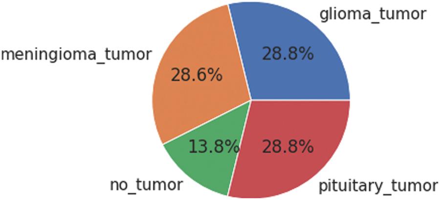
Figure 1: Each category’s proportion of the contrast-enhanced magnetic resonance imaging (CE-MRI) dataset
This research proposes a novel Block-wise VGG19 for MRI brain tumor detection and classification. It consists of a VGG19 feature extractor, and these features are further passed to BW-VGG19 architecture as input by freezing its initial layers and only training the fully connected layer. BW-VGG19 unfreezes all its layers with an already trained, fully connected layer and retrains the whole network. This way saves our computational resources and provides us the promising result to conquer future endeavors. The major contributions of the applied model are given below:
1. Implementation of fine-tuned Block-Wise VGG19 (BW-VGG19) architecture. In this method, a pre-trained VGG19 is fine-tuned with CNN architecture in the block-wise mechanism to enhance the system`s accuracy.
2. As a dataset preprocessing initially the dataset is made noise-free by using a histogram equalizer and removing duplications and missing values with CNN techniques.
The rest of this paper is organized as follows. We describe related work in Section 2. The detailed procedure of the proposed method is presented in Section 3. The datasets and evaluation criteria are presented in Section 4. Finally, Section 5 concludes the paper.
Mishra et al. [16] effectively achieved the best result for brain tumor classification by using wavelet transforms and a support vector machine. Everingham et al. [17] implemented CNNs on image classification and detection datasets and achieved the best results. Cheng et al. [18] implemented an adaptive spatial division method to enlarge tumor regions as a region of interest and then split them into sub-regions. The intensity histogram, gray-level co-occurrence matrix, and bag-of-words model-based features were extracted, and the ring-form partitioned method generated the accuracy of 87.54%, 89.72%, and 91.28%. Ismael et al. [19] proposed a method and attained 91% accuracy; they classify Meningioma, Glioma, and pituitary. Statistical features were extracted from MRI and two dimensional (2D) Gabor filter. Backpropagation was used to train multilayer perceptron neural networks for classification purposes. Kumar et al. [20] used fractional and multi-fractional dimension algorithms for a feature and essential feature extraction. Brain tumor detection performance was enhanced using machine learning based on backpropagation and a classification system was proposed.
Setio et al. [21] extracted the patches from particular points of nodule candidates using multiple streams of 2D CNNs. The information obtained from these multiple streams is then integrated to identify the pulmonary nodule. Thus, the proposed architecture for this recognition was based on multi-view convolutional networks. The results with the CNN experiment achieved 98.51% accuracy on training sets by implementing five different CNN architectures the architecture numbered 2 performed better, containing a Rectified Linear Unit (ReLU) layer and 64 hidden neurons max-pool two convolutional layers. Ayyoub et al. [22] use MATLAB and ImageJ to classify the MRIs into benign and malignant tissues; almost ten different features are extracted from MRI images to detect brain tumors. Parihar [23] proposed a CNN-based method involving preprocessing to obtain intensity normalization. Classification is performed using CNN architecture, and post-processing involves classifying the data as a tumor or not.
Zhu et al. [24] utilized two publicly available datasets and two deep learning models that classify tumors into meningioma, glioma, and pituitary tumors, and the second model assigned the grading to Glioma as Grade II, III, and IV. 16 layered CNN was used; the first model achieved 96.13%, while the second model achieved 98.7% accuracy. Ismael et al. [25] utilized CE-MRI very small dataset and experimented to find out the percentage of occurrence of three types of tumor meningioma, glioma, and pituitary tumor, achieving 45%, 15%, and 15% rates, respectively. Abdalla et al. [26] experimented with used a website named whole-brain atlas to obtain an MRI dataset. The preprocessing was applied to the available dataset, and the segmentation process was further carried out. A statistical approach was used for the feature extraction purpose, and a computer-aided detection system named the artificial neural network (ANN) model was proposed. MRI dataset was used as input to propose a system to classify the tumor or non-tumor images. The proposed method achieved 99% and 97.9% accuracy and sensitivity, respectively.
Vinoth et al. [27] proposed a CNN-based programmed division strategy to detect low and high-grade tumors. Based on the parameters and results obtained, an efficient support vector machine (SVM) is applied for the classification of benign and malignant tumors. Rehman et al. [28] performed a study based on transfer learning and CNN architecture to classify the brain tumor. For the application of transfer learning, they utilize ImageNet as the base dataset and Figshare as the target dataset to classify the glioma, meningioma, and pituitary. To identify the type of tumor AlexNet, GoogLeNet, and VGGNet, three deep CNN architectures were implemented on MRI images of the target dataset. The discriminative visual and pattern features were extracted from MRI images using Fine-tune and freeze transfer learning techniques. Swati et al. [29] used transfer learning and fine-tuning to propose a block-wise fine-tuning strategy for brain tumor image classification. T1 as weighted contrast-enhanced magnetic resonance images standard dataset used to train the model. Comparison of results with traditional machine learning and deep learning CNN-based methods; under five-fold cross-validation, the proposed method achieved 94.82% accuracy.
Ahmed et al. [30] conducted a study to predict survival time in the case of glioblastoma brain tumor and explored feature learning and deep learning methods on MRI images obtained from the ImageNet dataset, and deep CNN was pre-trained on the dataset. Training a large dataset to models increases complexity; transfer learning helps fine-tune the already trained models to a new task. The pre-trained CNN on a large dataset, and then the survival time prediction was carried out by transferring the pre-trained features. The flair sequence achieved 81.8% predictive accuracy.
To overcome the problem faced in brain tumor analysis a novel Block-wise VGG19 for MRI brain tumor detection and classification is proposed in this research. It consists of a VGG19 feature extractor, and these features are further passed to BW-VGG19 architecture as input by freezing its initial layers and only training the fully connected layer. BW-VGG19 unfreezes all its layers with an already trained, fully connected layer and retrains the whole network.
The overall structure of the methodology is explained in this section. The parameters used in the proposed fine-tuning process during the execution are explained below. The methodology workflow in Fig. 6 consists of two steps: dataset collection methods and information; dataset preprocessing includes four sub-steps known as cleaning, noise removal, resizing, and dataset distribution in test, train, and validation sets. The second and final step is feeding preprocessed data to the pre-trained CNN model. This model forwards its output for the fine-tuning of the pre-trained CNN model. The final value is forwarded to the proposed block-wise VGG19 model for the model execution to get the required results.
The freely accessible CE-MRI dataset (https://figshare.com/articles/dataset/brain_tumor_dataset/1512427) has been used in this work. The dataset consists of 2-dimensional images with a large slice gape. The dataset was collected from 2005 to 2020 from different hospitals in China. The dataset consists of four tumor classes glioma, meningioma, pituitary, and no tumor as shown in Fig. 1. A glioma tumor is a common brain tumor that originates in the glial tissues surrounded by neurons. In contrast, meningioma is a tumor that arises from meninges tissues surrounding the brain and spinal cardinal system. A pituitary tumor is due to the abnormal growth of pituitary glands in the back of the nose. The size of each image in the dataset is 512 x 512 pixels, as shown in Fig. 2. The CE-MRI dataset was separated into training 70%, validation 15%, and testing 15% to train the BW-VGG19 model for brain tumor segmentation. The description of the dataset is given below in Tab. 1.
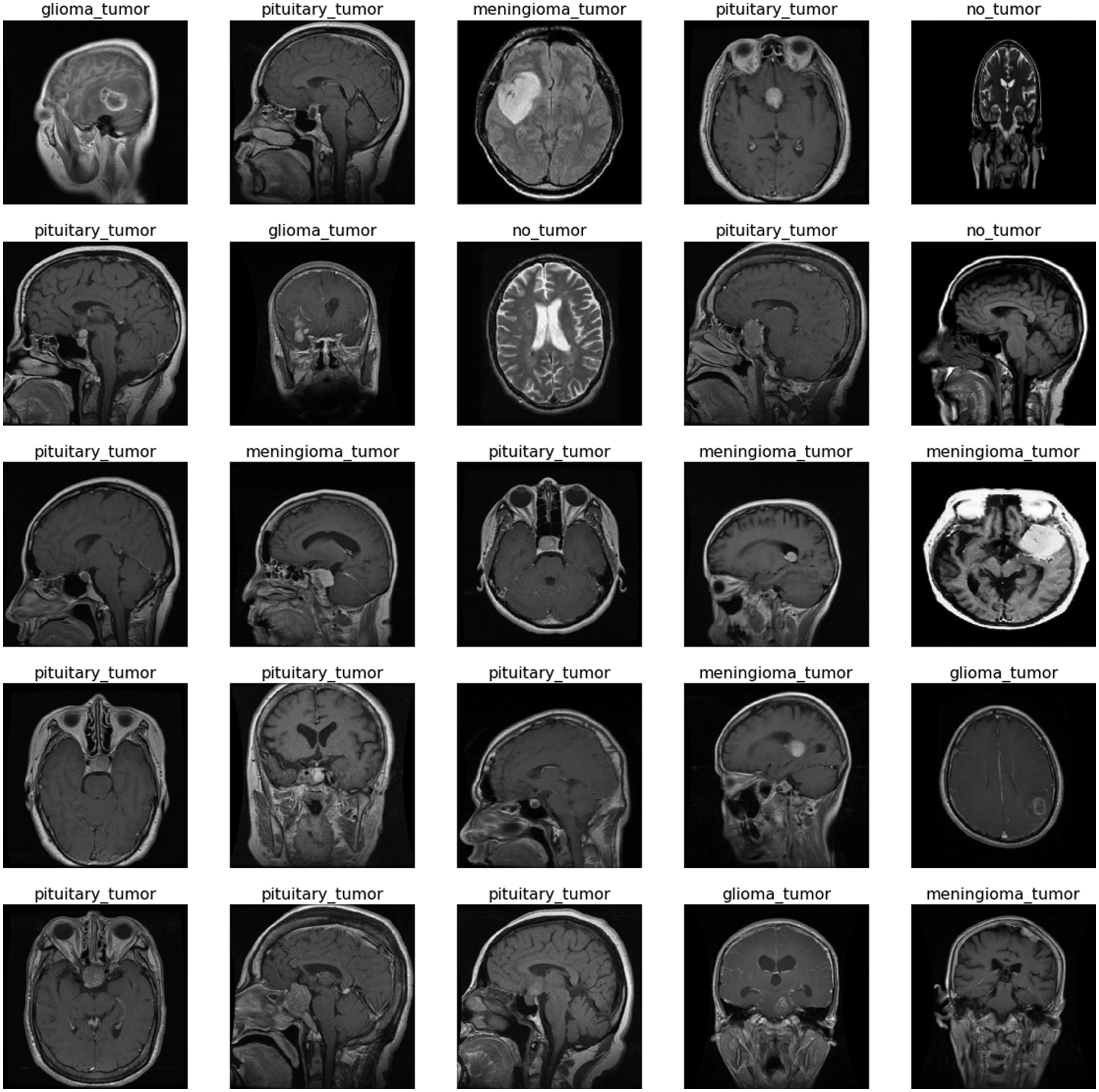
Figure 2: Sample images of contrast-enhanced magnetic resonance imaging (CE-MRI) dataset

The images in the dataset are 2-dimensional with 512 x 512 pixels, as shown in Fig. 2. The dataset is checked with duplication, missing values, label name, and extension during the cleaning. Moreover, all the images are made noise-free by using a histogram equalizer and segmentation process. In this work, the images are directly fed to the convolutional neural network, and the kernel is applied to resize the images. The results are highly dependent on these values. However, these values are not fixed and vary according to the image pixel sizes. These intensity variations are handled through normalization [31]. So before giving values to the CNN model for prediction and classification, all the values are normalized, having the same size range. Now the size of the images is 224 x 224 after normalization and resizing. In this way, the training process speeds up by resizing images and requires less memory for the prediction and classification of MRI images.
3.3 Convolutional Neural Network (CNN) Training
The training process of the CNNs is in a feed-forward manner beginning with the input layer and ending with the classification layer. On the other hand, the reverse process starts from classification to the first convolutional layer. The value of neuron I in layer J takes input from neuron K in the forward fashion calculated in Eq. (1). The output is calculated with the help of the nonlinear ReLU function, as shown in Eq. (2).
IP indicates input, OP as output, W is weight, and b neuron number.
All the neurons use Eqs. (1) and (2) to take the input value and create output results to form the nonlinear activation function. The pooling layer uses the kernel (r) sliding window to collect the results to take the maximum average values of the features.
The SoftMax function calculates the final layer classification value for each tumor type, as shown in Eq. (3).
The backpropagation cost function minimizes the unknown weights W, as shown in Eq. (4).
Here S is the training set sample,
Here
3.4 Fine-Tuning of Pre-Trained CNN
Throughout the training process, the weighted parameters for the CNN layers are in the condition of updating every time. The VGG19 pre-trained model is used for the weights handling of fine-tuning architecture. The VGG19 model contains sixteen convolutional layers tracked by one pooling layer. Each layer has different parameters and weights, as shown in Fig. 3. The convolutional layer is applied for feature extraction, the fundamental element of convolutional neural networks [32]. This layer contains different filters to extract features. The output and size of this layer are calculated using Eq. (6) and Eq. (7), respectively, where
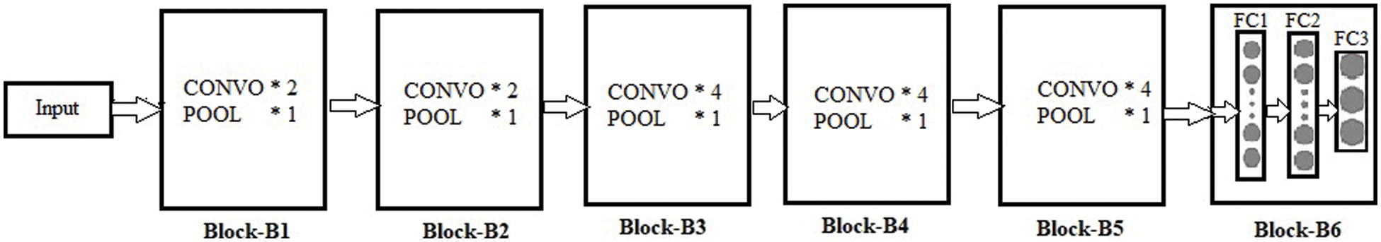
Figure 3: Proposed block-wise VGG19 (BW-VGG19) architecture
The pooling layer is frequently used after every convolutional layer in a convolutional neural network. This layer handles the parameters and is responsible for overfitting. Various pooling layers perform different functions (e.g., max, min, and average); the most frequently used layer is max pooling [33]. The size and output of the pooling layer are calculated using Eqs. (8) and (9), respectively, where x is the output and p denotes the pooling region.
In the end, three fully connected layers are added for the fine-tuning process. The strategy of layer-wise fine-tuning is more difficult because it takes more time to add a layer every time for iteration. As in the VGG19 network, we need to fine-tune nineteen layers.
Moreover, a minor enhancement in results has been observed during the layer base fine-tuning adoption. Thus, the VGG19 architecture is split into block-wise fine-tuning, as shown in Fig. 3. The fine-tuning is the multiple-step process as given below:
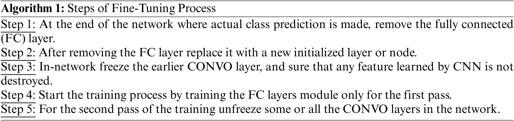
3.5 Block-Wise VGG19 (BW-VGG19) Architecture
The VGG19 trained model is fine-tuned in the block-wise mechanism. The fine-tuning process starts from the last block and freezes the other blocks by fixing the learning rate. The previous layer in this network contains the general features; the last layer emphasizes the domain-related topographies due to the features’ low-level format. We start fine-tuning from the top-level block to evaluate the domain-related topographies of brain tumors.
Fig. 4 shows the block-wise distribution of the layers for the fine-tuning process. Fig. 4A shows the original Block-Wise VGG19 (BW-VGG19) network consisting of nineteen CONV layers with each POOL layer and three FC layers. Moreover, Fig. 4B explains the removal of the FC layer head and considers the POOL layer as the feature extractor. On the other hand, in Fig. 4C old FC head is replaced with the FC head for the tuning process.
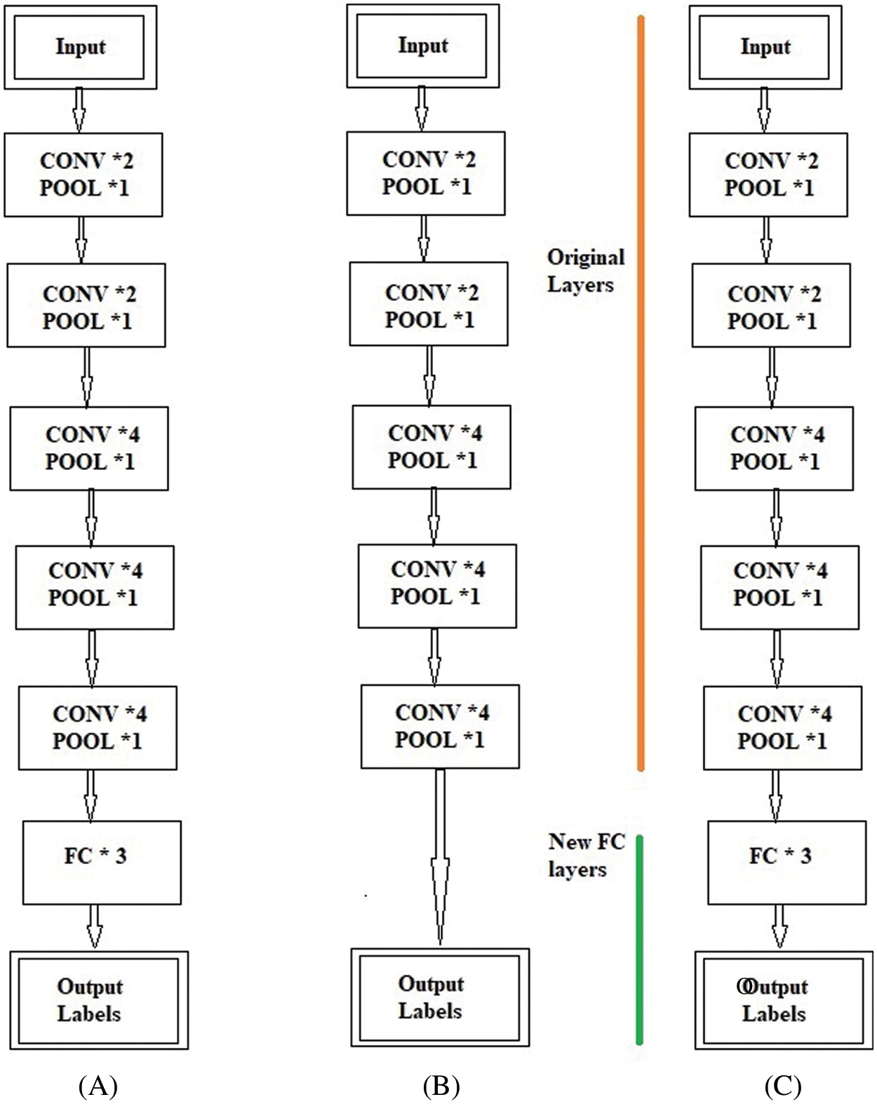
Figure 4: (A) Original VGG19 architecture (B) Removing of fully connected (FC) layer and considering pool layer as a feature extractor (C) Fully connected (FC) head substituting with new fully connected (FC) head
The freezing and unfreezing process for the BW-VGG19 is shown in Fig. 5. In Fig. 5E, the earlier layers of the BW-VGG19 network are in a frozen state. At this level, only the FC layer is in the state of training. Fig. 5F shows that the earlier layers of the BW-VGG19 network are released as unfreeze mood and start training for the whole network.
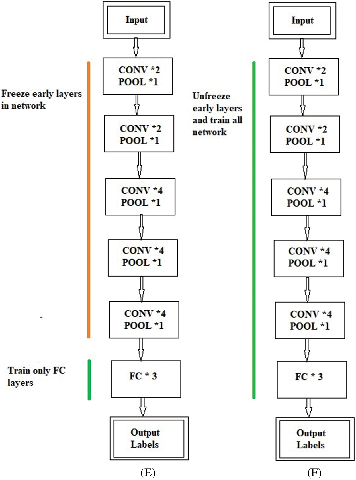
Figure 5: (E) Freeze the earlier layer and train only the fully connected (FC) layer (F) Unfreeze the earlier layer and train all the network
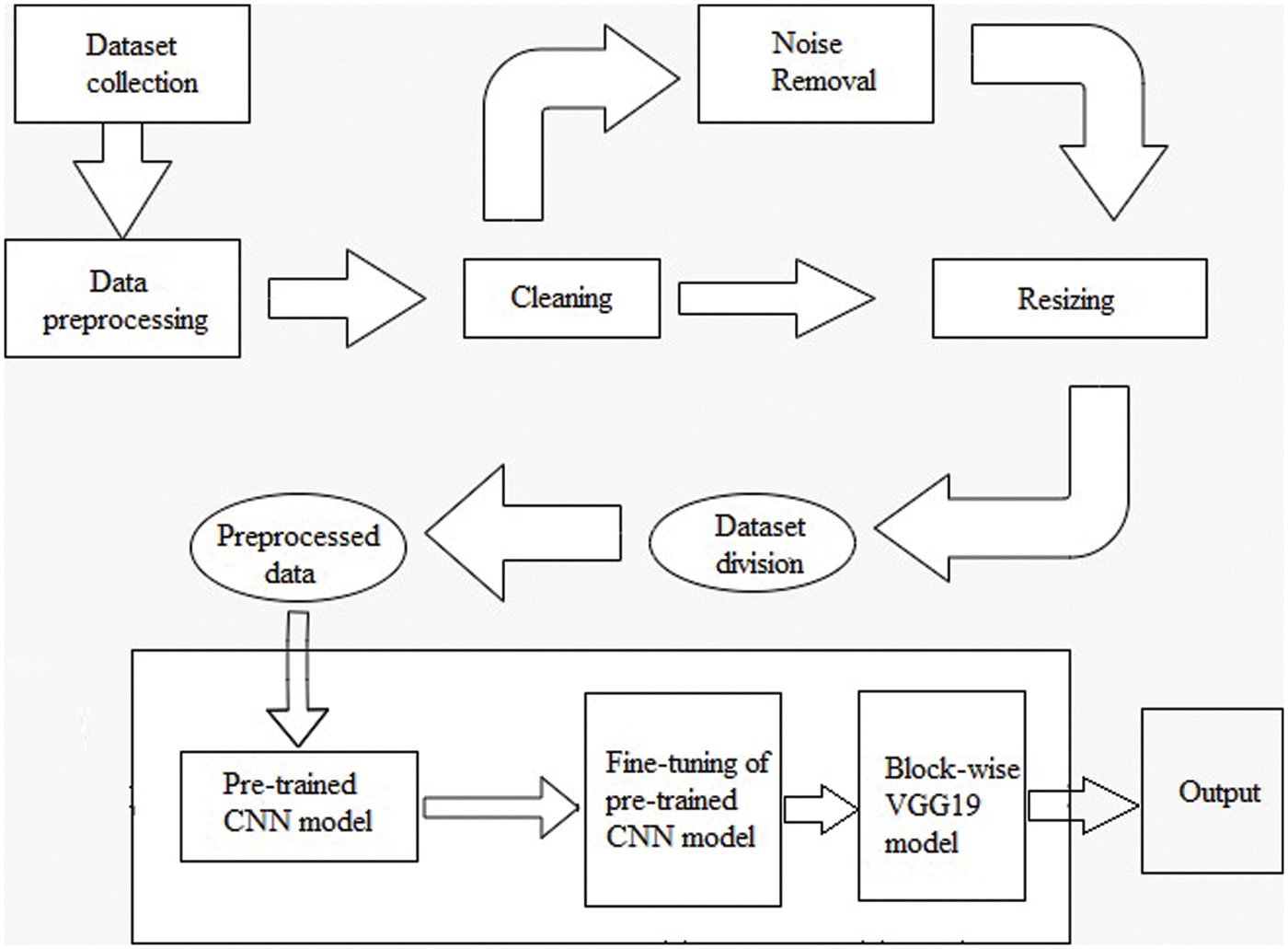
Figure 6: Methodology of workflow
This work described the experimental results achieved from fine-tuning and BW-VGG19. The anticipated fine-tuning and BW-VGG19 model was implemented in python on the computer system having GPU 6GB GTX1060, Core i7, 8th generation with RAM 16 GB to calculate brain tumor results.
The dataset consists of four classes Glioma images 826; Meningioma images 822; Pituitary images 827, and No Tumor 395 images. The CE-MRI dataset is divided into training 70%, validation 15%, and testing 15% to train the BW-VGG19 model for brain tumor segmentation. We have used Image Data Generator to generate batches of tensor images taking target size= (224, 224), color mode=’rgb’, class mode="categorical”, batch size = 32, and shuffle=False. Adam optimizer with learning rate 1e-4 and 10 epochs have been adopted for model training. To train the fine-tuning and BW-VGG19, the preprocessed dataset is fed to the proposed training process to get the required results. At this stage, many parameters are used with the proposed fine-tuning and BW-VGG19 architecture.
The test dataset from the preprocessing data phase is fed into the proposed model in the same layout as the training dataset once the model has been built. It is determined how accurate the classification or prediction is. The better the model, the closer it comes to a hundred percent accuracy. It also uses different parameters.
The proposed fine-tuning and BW-VGG19 for brain tumor classification and detection are evaluated with the help of different statistical equations given below from Eqs. (10)–(13). True positive is the correctly classified images known as Tp; a true negative is the negative classified images represented as Tn, Fp means the number of positively incorrect classified images. The Fn represents the total of negatively classified images. The statistical values sensitivity, accuracy rate, specificity, and precision were used to measure the ‘model’s output.
4.4 Results with Convolutional Neural Network (CNN) Model
Fig. 7 shows the CNN model confusion matrix for the four-class classification of the test dataset. The test dataset consists of four tumor classes glioma, meningioma, pituitary, and no tumor. The numbers in the boxes of the confusion matrix show the overall number of images used for the classification purpose. Fig. 8 displays the graphical demonstration of accuracy and loss for training and validation. The statistical values are also shown in Tab. 2 with average precision: 0.89, recall: 0.88, and F1-score: 0.88 values.

Figure 7: Convolutional neural network (CNN) model four-class classification confusion matrix for the test dataset

Figure 8: Graphical demonstration of training and validation accuracy and loss

The resultant confusion matrix of the VGG16 model is also presented in Fig. 9 to classify the test dataset into four classes of tumors glioma, meningioma, pituitary, and no tumor. The numbers in the boxes of the confusion matrix show the total number of images for classification and missed classification values. Fig. 10 shows the graphical demonstration of accuracy and loss for training and validation of VGG16. The mathematical values are also shown in Tab. 2, with an average of 0.87 values for precision, recall, and F1-score values, respectively.
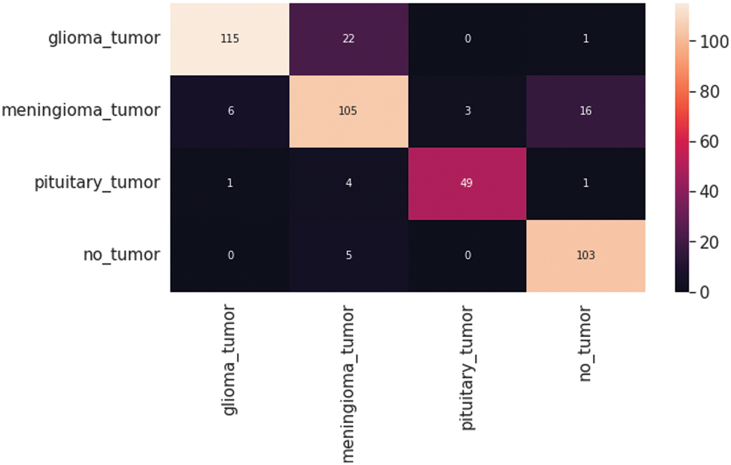
Figure 9: VGG16 Model four-class classification confusion matrix for the test dataset
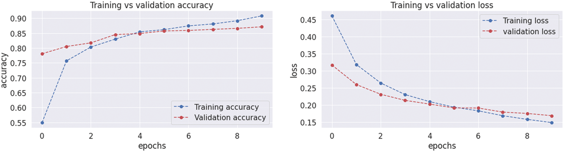
Figure 10: Graphical demonstration of training and validation accuracy and loss
The VGG19 model results are also depicted in Fig. 11 for the four-class classification with glioma, meningioma, pituitary, and no tumor for the test dataset. The numbers in the confusion matrix show the overall number of correctly and incorrectly classified images. Fig. 12 shows the graphical illustration of accuracy and loss for training and validation of VGG19. The statistical values are also shown in Tab. 2 with average precision: 0.92, recall 0.93, and F1-score: 0.93 values.
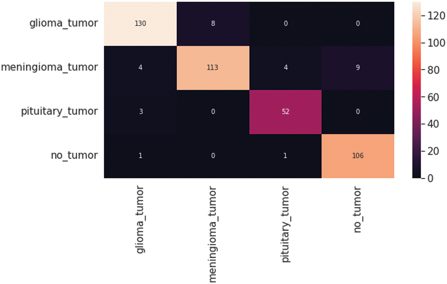
Figure 11: VGG19 model four-class classification confusion matrix for the test dataset
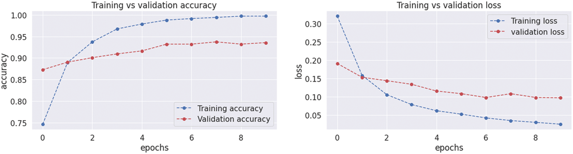
Figure 12: Graphical demonstration of training and validation accuracy and loss
4.7 Results with Block-Wise VGG19 (BW-VGG19) Model
The BW-VGG19 model results are also depicted in Fig. 13 for the four-class classification with glioma, meningioma, pituitary, and no tumor for the test dataset. The numbers in the confusion matrix show the overall number of correctly classified and incorrectly classified images. Fig. 14 shows the graphical demonstration of accuracy and loss for training and validation of BW-VGG19.

Figure 13: BW-VGG19 model four-class classification confusion matrix for the test dataset
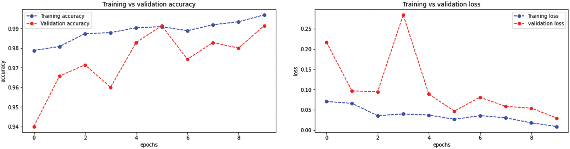
Figure 14: Graphical demonstration of training and validation accuracy and loss
The statistical values are also shown in Tab. 2 with average precision: 0.92, recall 0.93, and F1-score: 0.93 values for the VGG19 model. On the other hand, Tab. 2 also shows the average 0.87 values for precision, recall, and F1-score for the VGG19 model, and also for CNN model shows the average values for precision 0.89, recall 0.88, and F1-score 0.88.
Tab. 3 compares all the accuracy values for all the applied models below. The proposed BW-VGG19 architecture shows the best accuracy of 0.98% due to its block-wise structure. The other existing approaches show the lowest accuracy. The accuracy for other methods on the same dataset is CNN model: 0.89%, VGG16:0.86%, and VGG19 is 0.93%.

This research proposes a fine-tuned Block-Wise VGG19 (BW-VGG19) architecture. In this approach, a pre-trained VGG19 is fine-tuned in the block-wise mechanism to enhance the diagnosis accuracy. The publicly accessible CE-MRI dataset was used for this research. Our proposed method is straightforward and achieved an accuracy of 0.98%. The proposed method results are also matched with the existing CNN, VGG16, VGG19, and other approaches. The resultant statistical values represent that our proposed technique outperforms the accurate results compared to the other existing techniques on the CE-MRI dataset. As for directions, the proposed techniques would be used for other datasets and assist in the medical fields for the better analysis of brain tumors for the medical experts.
Funding Statement: Authors would like to acknowledge the support of the Deputy for Research and Innovation- Ministry of Education, Kingdom of Saudi Arabia for funding this research through a project (NU/IFC/ENT/01/014) under the institutional funding committee at Najran University, Kingdom of Saudi Arabia.
Conflicts of Interest: The authors declare that they have no conflicts of interest to report regarding the present study.
References
1. R. L. Siegel, K. D. Miller and A. Jemal, “Cancer statistics,” CA: A Cancer Journal for Clinicians, vol. 65, no. 1, pp. 5–29, 2015. [Google Scholar]
2. A. G. Sauer, R. L. Siegel, A. Jemal and S. A. Fedewa, “Current prevalence of major cancer risk factors and screening test use in the United States: Disparities by education and race/ethnicity,” Cancer Epidemiology and Prevention Biomarkers, vol. 28, no. 4, pp. 629–642, 2019. [Google Scholar]
3. N. Abiwinanda, M. Hanif, S. T. Hesaputra, A. Handayani and T. R. Mengko, “Brain tumor classification using convolutional neural network,” International Federation for Medical and Biological Engineering, vol. 68, no. 1, pp. 183–189, 2019. [Google Scholar]
4. T. A. Abir, J. A. Siraji, E. Ahmed and B. Khulna, “Analysis of a novel MRI based brain tumor classification using probabilistic neural network (PNN),” International Journal of Scientific Research in Science, Engineering and Technology, vol. 8, no. 4, pp. 69–75, 2018. [Google Scholar]
5. A. Naseer, M. Rani, S. Naz, M. I. Razzak, M. Imran and G. Xu, “Refining Parkinson’s neurological disorder identification through deep transfer learning,” Neural Computing and Applications, vol. 32, no. 3, pp. 839–854, 2020. [Google Scholar]
6. R. Núñez-Martín, R. Cubedo Cervera and M. Provencio Pulla, “Gastrointestinal stromal tumour and second tumours: A literature review,” Medicina Clínica, vol. 149, no. 8, pp. 345–350, 2017. [Google Scholar]
7. J. Kleesiek, A. Biller, G. Urban, U. Kothe, M. Bendszus et al., “Ilastik for multi-modal brain tumor segmentation,” in Proc. Medical Image Computing and Computer-Assisted Intervention on Multimodal Brain Tumor Image Segmentation, Boston, MA, USA, pp. 12–17, 2014. [Google Scholar]
8. R. Meier, S. Bauer, J. Slotboom, R. Wiest and M. Reyes, “Appearance-and context-sensitive features for brain tumor segmentation,” in Proc. Medical Image Computing and Computer-Assisted Intervention on Multimodal Brain Tumor Image Segmentation, Boston, MA, USA, pp. 20–26, 2014. [Google Scholar]
9. J. Long, E. Shelhamer and T. Darrell, “Fully convolutional networks for semantic segmentation,” in Proc. 2015 IEEE Conf. on Computer Vision and Pattern Recognition, Boston, MA, USA, pp. 3431–3440, 2015. [Google Scholar]
10. F. J. Díaz-Pernas, M. Martínez-Zarzuela, M. Antón-Rodríguez and D. González-Ortega, “A deep learning approach for brain tumor classification and segmentation using a multiscale convolutional neural network,” Healthcare (Basel), vol. 9, no. 2, pp. 153–166, 2021. [Google Scholar]
11. J. Cheng, “Brain tumor dataset.,” figshare, 17-April- 2022. Available: https://figshare.com/articles/dataset/brain_tumor_dataset/1512427. [Google Scholar]
12. L. von Baumgarten, D. Brucker, A. Tirniceru, Y. Kienast, S. Grau et al., “Bevacizumab has differential and dose-dependent effects on glioma blood vessels and tumor cells,” Clinical Cancer Research: An Official Journal of the American Association for Cancer Research, vol. 17, no. 19, pp. 6192–6205, 2011. [Google Scholar]
13. S. Ferluga, D. Baiz, D. A. Hilton, C. L. Adams, E. Ercolano et al., “Constitutive activation of the EGFR-STAT1 axis increases proliferation of meningioma tumor cells,” Neuro-oncology Advances, vol. 2, no. 1, pp. 08–19, 2020. [Google Scholar]
14. M. Satou, J. Wang, T. Nakano-Tateno, M. Teramachi, T. Suzuki et al., “L-Type amino acid transporter 1, LAT1, in growth hormone-producing pituitary tumor cells,” Molecular and Cellular Endocrinology, vol. 515, no. 1, pp. 110868–110930, 2020. [Google Scholar]
15. A. S. Razavian, H. Azizpour, J. Sullivan and S. Carlsson, “CNN features off-the-shelf: An astounding baseline for recognition,” in Proc. 2014 IEEE Conf. on Computer Vision and Pattern Recognition Workshops, Columbus, OH, USA, pp. 806–813, 2014. [Google Scholar]
16. S. K. Mishra and V. H. Deepthi, “Brain image classification by the combination of different wavelet transforms and support vector machine classification,” Journal of Ambient Intelligence and Humanized Computing, vol. 12, no. 6, pp. 6741–6749, 2021. [Google Scholar]
17. M. Everingham, S. M. A. Eslami, L. Van Gool, C. K. I. Williams, J. Winn et al., “The pascal visual object classes challenge: A retrospective,” International Journal of Computer Vision, vol. 111, no. 1, pp. 98–136, 2015. [Google Scholar]
18. J. Cheng, W. Huang, S. Cao, R. Yang, W. Yang et al., “Enhanced performance of brain tumor classification via tumor region augmentation and partition,” Public Library of Science One, vol. 10, no. 10, pp. 81–93, 2015. [Google Scholar]
19. M. R. Ismael and I. Abdel-Qader, “Brain tumor classification via statistical features and back-propagation neural network,” in Proc. 2018 IEEE Int. Conf. on Electro/Information Technology (EIT), Rochester, MI, USA, pp. 0252–0257, 2018. [Google Scholar]
20. A. Kumar, M. Ramachandran, A. H. Gandomi, R. Patan, S. Lukasik et al., “A deep neural network based classifier for brain tumor diagnosis,” Applied Soft Computing, vol. 82, no. 1, pp. 105528–105565, 2019. [Google Scholar]
21. A. A. A. Setio, F. Ciompi, G. Litjens, P. Gerke, C. Jacobs et al., “Pulmonary nodule detection in CT images: False positive reduction using multi-view convolutional networks,” Institute of Electrical and Electronics Engineers Transactions on Medical Imaging, vol. 35, no. 5, pp. 1160–1169, 2016. [Google Scholar]
22. M. Al-Ayyoub, G. Husari, O. Darwish and A. Alabed-Alaziz, “Machine learning approach for brain tumor detection,” in Proc. the 3rd Int. Conf. on Information and Communication Systems, New York, NY, United States, pp. 1–4, 2012. [Google Scholar]
23. A. S. Parihar, “A study on brain tumor segmentation using convolution neural network,” in Proc. 2017 Int. Conf. on Inventive Computing and Informatics (ICICI), Coimbatore, India, pp. 198–201, 2017. [Google Scholar]
24. H. Zhu, Y. Miao, Y. Shen, J. Guo, W. Xie et al., “The clinical characteristics and molecular mechanism of pituitary adenoma associated with meningioma,” Journal of Translational Medicine, vol. 17, no. 1, pp. 1–9, 2019. [Google Scholar]
25. S. A. Abdelaziz Ismael, A. Mohammed and H. Hefny, “An enhanced deep learning approach for brain cancer MRI images classification using residual networks,” Artificial Intelligence in Medicine, vol. 102, no. 1, pp. 101779–101786, 2020. [Google Scholar]
26. H. E. M. Abdalla and M. Y. Esmail, “Brain tumor detection by using artificial neural network,” in Proc. 2018 Int. Conf. on Computer, Control, Electrical, and Electronics Engineering (ICCCEEE), Khartoum, Sudan, pp. 1–6, 2018. [Google Scholar]
27. R. Vinoth and C. Venkatesh, “Segmentation and detection of tumor in MRI images using CNN and SVM classification,” in Proc. 2018 Conf. on Emerging Devices and Smart Systems (ICEDSS), Tiruchengode, India, pp. 21–25, 2018. [Google Scholar]
28. A. Rehman, S. Naz, M. I. Razzak, F. Akram and M. Imran, “A deep learning-based framework for automatic brain tumors classification using transfer learning,” Circuits Systems Signal Process, vol. 39, no. 2, pp. 757–775, 2020. [Google Scholar]
29. Z. N. K. Swati, Q. Zhao, M. Kabir, F. Ali, Z. Ali et al., “Brain tumor classification for MR images using transfer learning and fine-tuning,” Computerized Medical Imaging and Graphics: The Official Journal of the Computerized Medical Imaging Society, vol. 75, no. 1, pp. 34–46, 2019. [Google Scholar]
30. K. B. Ahmed, L. O. Hall, D. B. Goldgof, R. Liu and R. A. Gatenby, “Fine-tuning convolutional deep features for MRI based brain tumor classification,” in Proc. Medical Imaging 2017: Computer-Aided Diagnosis, Orlando, Florida, United States, pp. 613–619, 2017. [Google Scholar]
31. J. -F. Mangin, J. Lebenberg, S. Lefranc, N. Labra, G. Auzias et al., “Spatial normalization of brain images and beyond,” Medical Image Analysis, vol. 33, no. 1, pp. 127–133, 2016. [Google Scholar]
32. E. A. Smirnov, D. M. Timoshenko and S. N. Andrianov, “Comparison of regularization methods for ImageNet classification with deep convolutional neural networks,” Arctic and Antarctic Scientific Research Institute Procedia, vol. 6, no. 1, pp. 89–94, 2014. [Google Scholar]
33. H. J. Jie and P. Wanda, “RunPool: A dynamic pooling layer for convolution neural network,” International Journal of Computational Intelligence Systems, vol. 13, no. 1, pp. 66–76, 2020. [Google Scholar]
34. R. R. Wahid, F. T. Anggraeni and B. Nugroho, “Brain tumor classification with hybrid algorithm convolutional neural network-extreme learning machine,” International Journal of Computer, Network Security and Information System, vol. 3, no. 1, pp. 29–33, 2021. [Google Scholar]
35. P. Afshar, K. N. Plataniotis and A. Mohammadi, “Capsule networks for brain tumor classification based on MRI images and coarse tumor boundaries,” in Proc. 2019 IEEE Int. Conf. on Acoustics, Speech and Signal Processing (ICASSP), Brighton, UK, pp. 1368–1372, 2019. [Google Scholar]
 | This work is licensed under a Creative Commons Attribution 4.0 International License, which permits unrestricted use, distribution, and reproduction in any medium, provided the original work is properly cited. |