Computers, Materials & Continua DOI:10.32604/cmc.2022.032086
Article

An Image Localization System Based on Single Photon

Yanyi Wu1, Xiaoyu Li2, Qinsheng Zhu1,*, Xiaolei Liu2, Hao Wu1 and Shan Yang3

1School of Physics, University of Electronic Science and Technology of China, Chengdu, 610054, China
2School of Information and Software Engineering, University of Electronic Science and Technology of China, Chengdu, 610054, China
3Department of Chemistry, Physics and Atmospheric Sciences, Jackson State University, Jackson, USA
*Corresponding Author: Qinsheng Zhu. Email: zhuqinsheng@uestc.edu.cn
Received: 06 May 2022; Accepted: 09 June 2022

Abstract: As an essential part of artificial intelligence, many works focus on image processing which is the branch of computer vision. Nevertheless, image localization faces complex challenges in image processing with image data increases. At the same time, quantum computing has the unique advantages of improving computing power and reducing energy consumption. So, combining the advantage of quantum computing is necessary for studying the quantum image localization algorithms. At present, many quantum image localization algorithms have been proposed, and their efficiency is theoretically higher than the corresponding classical algorithms. But, in quantum computing experiments, quantum gates in quantum computing hardware need to work at very low temperatures, which brings great challenges to experiments. This paper proposes a single-photon-based quantum image localization algorithm based on the fundamental theory of single-photon image classification. This scheme realizes the operation of the mixed national institute of standards and technology database (MNIST) quantum image localization by a learned transformation for non-noise condition, noisy condition, and environmental attack condition, respectively. Compared with the regular use of entanglement between multi-qubits and low-temperature noise reduction conditions for image localization, the advantage of this method is that it does not deliberately require low temperature and entanglement resources, and it improves the lower bound of the localization success rate. This method paves a way to study quantum computer vision.

Keywords: MNIST data; single-photon; quantum computing; image localization

1  Introduction

In recent decades, with the development of information technology and computer hardware, the computing power of computers has been dramatically improved. The current application of artificial intelligence in various fields makes our life more intelligent. Image processing is widely studied as an essential branch of computer vision, such as image classification, object recognition, and semantic segmentation. However, the explosive growth of today’s data makes the performance of classical computers unable to meet the status quo of image processing. Therefore, numerous researchers invest in exploring efficient computer performance, such as very large scale integration technology and microprocessor technology [1], massively parallel processing systems [2], determinantal point processes [3]. Although these methods effectively improve the current situation, they are still dwarfed by the further increase of the data.

As a new heuristic theory and technology, quantum computing has attracted significant attention in some fields in recent years. It benefits from quantum computers’ powerful parallel computing capabilities [4]. The original idea of quantum computing came in 1982, Feynman proposed to use quantum mechanics-based computers to solve a particular problem more efficiently than traditional computers [5]. Then in 1994, Shor proposed to use a polynomial-time algorithm to solve large number factorization [6]. For quantum computing, the proposal of this algorithm is a milestone leap, and it has brought significant progress to quantum computing. Since then, the fields of quantum computing, information technology, and computer science have gradually moved towards mutual integration and mutual progress. The study of Rènyi Discord [7], the quantum many-body problem [8], quantum state tomography [9], and quantum correlations [10] based on machine learning have gained attention in the last few years.

Sometimes in some image processing scenarios, we usually need to identify [11], classify [12] and locate the image [13] which is the process of identifying and searching small images within a large image. Nowadays, quantum computing is applied in image localization processing. At the same time, many quantum image localization algorithms have been proposed, and their efficiency is theoretically higher than some traditional classical algorithms. Such as, the Massachusetts Institute of Technology laboratory proposed a quantum-based localization system, which theoretically proved that quantum entanglement could improve localization accuracy [14]. Later, Nan Jiang proposed a quantum image localization algorithm, which modifies the probability of pixels so that the target pixel is measured with a higher probability [15]. Recently, Muyu Li proposed a real-time multi-target tracking technology based on deep learning [16]. Although these technologies about quantum image localization obtain some exciting results theoretically, it is still difficult to realize it on computer hardware. Because the quantum gate in quantum computing hardware is easily affected by the environment [17], which arouses decoherence and dissipation. As one of the carriers of quantum computing, the single-photon could solve this problem. Simultaneously, we can improve the accuracy by adjusting the parameters of some linear optics. So, Thomas Fischbacher and Luciano Sbaiz proposed a single-photon image classification method [18]. This method can be implemented at room temperature and improved the lower resolution limit. However, they only study images’ classification and do not involve image localization. Therefore, this motivates our interest in image localization through quantum computing and single-photon technology.

This paper shows a single-photon-based quantum image localization method. Firstly, we perform a preprocessing on the image data, including but not limited to encoding labels, normalizing image pixels, generating a quantum state, etc. Secondly, a learned transformation is introduced to redistribute the amplitudes that make up the spatial part of the photon’s wave function [19]. Finally, we update the parameters to optimize the quantum image localization model and further improve the accuracy of our single-photon quantum localization results.

This paper is organized: The framework of the localization system is described in Section 2. Section 3 shows an example that describes the definition of the localization on the specific MNIST images in mathematics. In Section 4, we give three cases for experimental analysis of quantum image localization and draw some conclusions. In Section 5, we conclude this paper.

2  The Framework of Localization System

Here, we establish an overall framework for a quantum image localization system (QILS) to achieve single-photon image localization, as shown in Fig. 1. The single-photon light source illuminates the image to be positioned, the U-transformation obtained by the conversion unit acts on the data arranged in rows (or columns), and the single-photon detector [20] detects the transformed data to obtain the prediction of the image position. After this learned transformation, the accuracy of the predicted position in this paper is steadily improved.

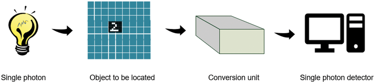
Figure 1: The frame diagram of QILS. The QILS consists of a single photon source, a localization image, a conversion unit and a single photon detector. The front of the frame is a single-photon source that emits a single photon to illuminate the image. After that is the big image with the localization map, the area of number “2” is the small image to be positioned. Then there is a conversion unit, which is used to improve the localization accuracy of the entire model. The rear of the frame diagram is a single-photon detector to obtain localization information

3  Single-Photon Quantum Image Localization Experiments on MNIST Images

3.1 Experimental Background

Inspired by Thomas Fischbacher and Luciano Sbaiz, we propose a new theory to realize image localization (the more details see Supplementary Files). Based on the above theory and considering the three cases and reasons: ideal situation, the noise-only situation, and the environmental attack situation to conduct relevant experiments.

•   Reason for the ideal situation: When doing experiments, ignoring all external factors that are not relevant to the experiment helps to detect whether the algorithm is achievable.

•   Reason for the noise-only situation: Due to the development of image positioning in various fields, its accuracy becomes particularly essential, such as computed tomography (CT) images in the medical field [21], alien images in aerospace [22] and road surveillance images [23]. The localization accuracy of these images needs to be guaranteed, but there will be some noise in the image transmission process, resulting in blurred images. In reality, noise is introduced into the image during the transmission process for some reason, and low-quality images will affect the localization [24].

•   Reasons for environmental attack situations: In practical application scenarios, modern learning algorithms may be subject to various adversarial attacks, including poisoning during model updates, model stealing, and test data evasion attacks [25]. Such attacks can be catastrophic as the application of machine learning algorithms grows in society.

3.2 Experiment Procedure

In this paper, we use the TensorFlow framework, which can be used for various machine learning and deep learning, such as speech recognition or image recognition [26]. It also uses Python 3.8 for Internet, web development, and artificial intelligence [27]. Fig. 2 shows the flow chart of the quantum image localization system. The detailed steps are shown as follows:

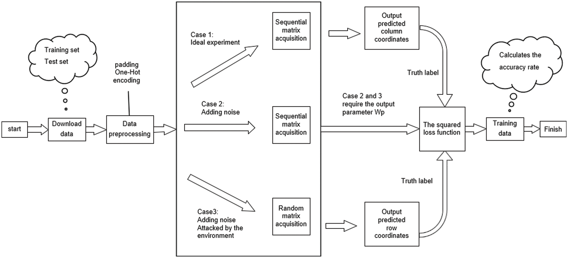
Figure 2: Program design flowchart of localization model

(1)   Prepare the image to be positioned based on the MNIST dataset [28]:

We call the original MNIST image a small image and the generated image localized to a large image. A number is randomly selected from the sequence of numbers 0–17 as the row label of the small image in the large image (Do the same for column label). In this way, each MNIST image will be put into a blank image of 504pixels×504pixels. For ease of calculation, each image will be compressed to a size of 28pixels×28pixels. And the label position of the image corresponding to the position to be predicted is (row, col).

(2)   The loading data stage:

   •   First, this paper divides the images containing MNIST data into two parts: a training set and test set. Each part contains 28pixels×28pixels grayscale images and corresponding position labels. Among them, there are 60,000 training sets and 10,000 test sets.

   •   After that, the divided test set and data set are randomly shuffled in batches, and then the image data of each batch is trained.

(3)   The preprocessing stage:

   •   Since the picture is a grayscale image containing handwritten numbers, its pixels are 28pixels×28pixels in size. We need to make the pixels one-dimensional, that is, become a vector784×1.

   •   The predicted position coordinates are (0, 0) to (18, 18). The M dimension needs to be divisible by the total number of positions C, that is, 784 needs to be divisible by 18. Since it is not divisible, the Hilbert space here needs to be filled to a larger Hilbert space. We extend vector 784×1 to 792×1 with 0.

   •   The coefficient of the photon quantum state is proportional to the square root of the picture’s brightness, and each element on the pixel with 28pixels×28pixels picture represents the brightness here. Therefore, in the preprocessing stage, it is necessary to take the square root of the brightness of each pixel and then normalize it to obtain the coefficient of the photon quantum state.

   •   One-Hot encoding is performed on the row and column labels of the image.

   •   In this stage, case 1 is fine as above, but cases 2 and 3 need to introduce noise. Simulation of noisy images: Add random numbers as noise to images containing predicted image locations [29]. The random here follows a standard normal distribution with a mean of 0 and a standard deviation of 1. The image after adding noise can be expressed in Fig. 3.

(4)   The predicting row or column stage:

   •   For case 1 (see Fig. 2): After the picture pixels are arranged in rows and filled into a one-dimensional vector of 792 pixels. Divide the vector 792 into 18 segments, each segment is a set of column vectors A. Then do the following operations on the vector A:

AAH=(a11⋯a1n⋮⋱⋮an1⋯ann)(1)

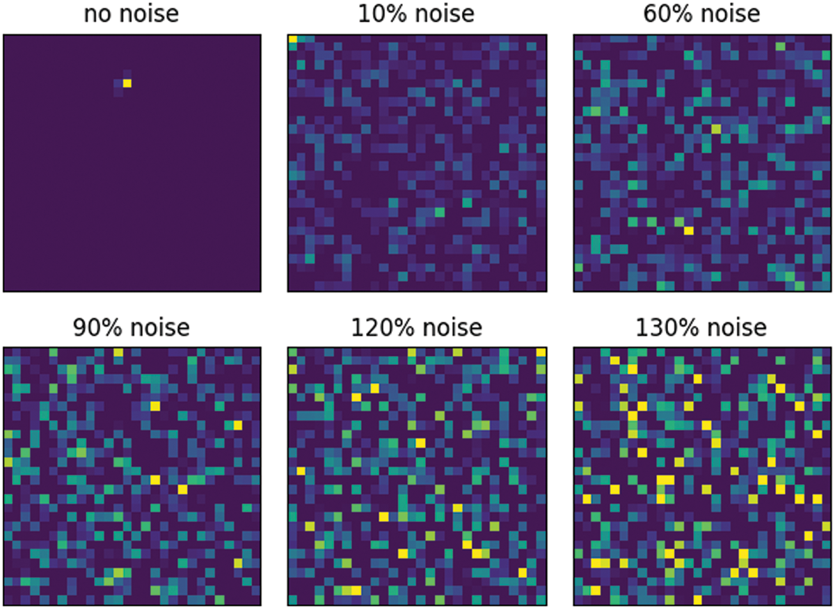
Figure 3: Images after adding different degrees of noise. The percentage in the picture is the level of random noise

The probability corresponding to this segment can be:

p=∑i=1n⁡aii(2)

By analogy, this operation is performed for each segment. And the probability of each segment is placed in an output list so that a list of numbers of predicted rows can be obtained. In the same way, after arranging the picture pixels in columns and filling them into a one-dimensional vector of 792 pixels, a list of numbers for the predicted column can be obtained after the above operations.

•   For case 2 (see Fig. 2): After adding random noise, we take the first 44 data from the row-wise 792-pixel data as the first segment. Then take the first 44 data from the remaining 748 as the second segment. Analogously, 18 segments can be obtained. For the first segment of column vector B, do the same as in the previous point:BBH. The probability corresponding to this segment can be:

p=∑i=1n⁡bii(3)

Similarly, this operation is performed for each segment, and the probability of each segment is placed in an output list so that a list of numbers of predicted rows can be obtained. In the same way, after arranging the picture pixels in columns and filling them into a one-dimensional vector of 792 pixels, a list of numbers for the predicted column can be obtained after the above operations.

•   For case 3 (see Fig. 2): To achieve the effect, the selected data is scrambled under the environmental attack. We randomly selected 44 data from the 792 pixels data arranged in rows as the first segment. Then randomly select 44 data from the remaining 748 pixels data as the second segment. Repeating this operation, we will get 18 segments with random data. For column vector C of the first segment, do the same as in the previous point:CCH. The probability corresponding to this segment can be:

p=∑i=1n⁡cii(4)

The probabilities obtained for each segment are put into an output list, which is a numerical list of predicted rows. Similarly, the picture pixels are arranged in columns and then filled into a one-dimensional vector of 792 pixels. After the above operations, the number list of the predicted columns can be obtained.

(5)   The training data stage:

The TensorFlow framework can access the entire calculation process, and it has a large number of built-in optimization algorithms. In this paper, an optimizer used a gradient descent algorithm is selected to update the value of the loss function and parameterWP. It should be noted that the parameter WP here is required by the learned transformation UP [30] in cases 2 and 3. The squared difference loss function:

loss(P,T)=∑in⁡(Pi−Ti)2(5)

Here P represents the predicted location label, and T represents the true location label. It can be seen that four main quantities directly affect the squared difference loss function, namely, One-Hot encodings corresponding to row labels and column labels and output sequences of predicted rows and columns. The indirect influence is the WP parameter required to learn the transformationUP.

Every 100 pictures are a batch. When the position of 100 pictures is predicted, the predicted localization result of each picture and the accuracy of the prediction of 100 pictures will be simulated.

4  Experiment and Result Analysis

4.1 Experiment

Under ideal conditions, we use a gradient descent optimizer to optimize the single-photon quantum image localization model. Fig. 4 shows the localization accuracy of this model without noise and attack. Experiments in this ideal situation can further reveal the inherent logical connection between objective phenomena and processes, and draw important conclusions. Through ideal experiments, the accuracy of the positioning system can be observed every 10 steps. When the number of training steps is 10, the localization accuracy of the model is 84%. When the number of training steps is 20, the localization accuracy of the model is 99%, and when the number of training steps is 30 or more, the localization accuracy of the model is 100%. Experiments have proved that this model is a perfect model for predicting the position of the image.

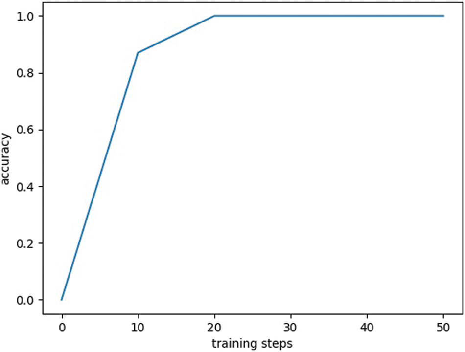
Figure 4: Location accuracy under ideal conditions. The abscissa of each image represents the number of training steps, and the ordinate represents the positioning accuracy under ideal conditions of the images in the dataset. The learning rate in the experiment is lr = 0.001

For noisy situations, add random numbers to the image to simulate positional noise. A single-photon quantum image localization model can predict the exact location of an image. The localization accuracy of the model in the presence of noise is shown in Fig. 5. When the number of training steps is 25, the localization accuracy of the model is 5%. When the number of training steps is 150, the localization accuracy of the model is 85%, and when the number of training steps is 400 or more, the localization accuracy of the model is about 99%. The observed localization accuracy is within the acceptable range.

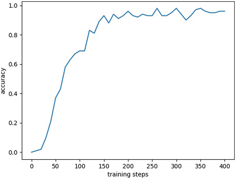
Figure 5: Location accuracy under noisy training conditions. The abscissa of each image represents the number of training steps, and the ordinate represents the positioning accuracy under noisy conditions of the images in the dataset. The learning rate in the experiment is lr = 0.001. With the increase of the number of training steps, the accuracy of image localization increases gradually and fluctuates until it becomes stable

If the environment attacks the quantum image localization model, the integrity of the learning process during the training stage will be compromised. In the case of adding noise, we use the operation of randomly selecting 44 data as a segment to simulate the situation where the model is attacked. The localization accuracy of the model with noise and environmental attacks is shown in Fig. 6. When the number of training steps is 250, the localization accuracy of the model is 50%. When the number of training steps is 750, the localization accuracy of the model is 87%, and when the number of training steps is 1700 or more, the localization accuracy of the model is about 99%. From this result, it can be observed that the single-photon quantum image localization model can still train well in complex situations.

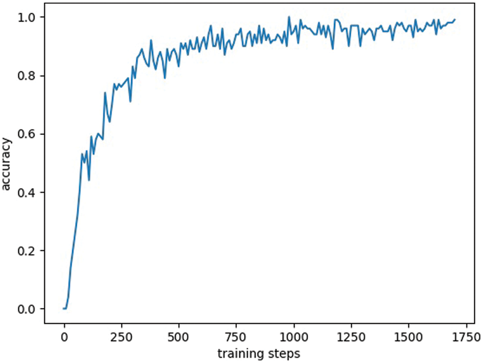
Figure 6: Location accuracy under noisy and random data training conditions. The abscissa of each image represents the number of training steps, and the ordinate represents the positioning accuracy under complex conditions of the images in the dataset. The learning rate in the experiment is lr = 0.001. With the increase of the number of training steps, the accuracy of image localization fluctuates gradually with the number of training steps

4.2 Result Analysis

Our model can obtain better image localization results by discussing the above three cases. These results stem from: 1. The performance indicators concerned in this paper are the possibility of correct localization and the output of the localization. 2. In model training, the squared difference loss function for gradient descent is used to achieve the optimal model. 3. When the program is compiled, the specific loss value of the squared loss function can be obtained every ten times of prediction position calculation. As the loss value of the squared difference loss function gets smaller and smaller, the predicted location result gets closer and closer to the correct location label.

Here, to show the relevant comparison of these three cases, we put the results in Tab. 1. The three cases are: the ideal situation is that there is no noise and the influence of environmental attacks, the picture itself is affected by noise, and the model is affected by environmental attacks. The number of training steps in the table represents the number of iterations to predict the position. It can be observed that under ideal conditions when the number of iterations reaches about 200, the accuracy rate reaches 100%; under the influence of noise alone, when the number of iterations reaches about 1000, the accuracy rate reaches 100%; when the picture is complicated, the number of iterations needs to reach more than 1700, and its accuracy rate can reach 100%. In any case, high localization accuracy will be achieved, but there are changes in the length of time and the number of iterations.

5  Conclusion

This paper proposes a quantum image localization method based on a single photon and studies the localization problem of single-photon and quantum computing for pictures containing MNIST images. Two main results are obtained: One is successful in establishing a new quantum image localization model based on the single-photon image classification method for the first time. The other is to introduce a transition matrix U in the quantum state of a single photon. Through theoretical analysis and numerical experiments, it is found that the conversion unit can improve the localization accuracy of the image. Most of the previous research on quantum image localization focused on a single environmental condition, lacking a comprehensive analysis of the system’s predictive ability under multiple physical conditions. This paper discusses the localization capability of QILS in three different situations, which has practical significance and excellent reference value for the application of quantum image localization. In general, this model helps us understand more complex quantum image localization systems and study high-dimensional image localization location characteristics.

Funding Statement: This work was supported by the National Key R&D Program of China, Grant No. 2018YFA0306703; Chengdu Innovation and Technology Project, No. 2021-YF05–02413-GX.

Conflicts of Interest: The authors declare that they have no conflicts of interest to report regarding the present study.

References

 1.  M. Abe, T. Mimura, N. Yokoyama and H. Ishikawa, “New technology towards GaAs LSI/VLSI for computer applications,” IEEE Transactions on Microwave Theory and Techniques, vol. 30, no. 7, pp. 992–998, 1982, https://doi.org/10.1109/TMTT.1982.1131188. [Google Scholar]

 2.  E. C. Bronson, T. L. Casavant and L. H. Jamieson, “Experimental application-driven architecture analysis of an SIMD/MIMD parallel processing system,” IEEE Transactions on Parallel and Distributed Systems, vol. 1, no. 2, pp. 195–205, 1990, https://doi.org/10.1109/71.80147. [Google Scholar]

 3.  C. Launay, A. Desolneux and B. Galerne, “Determinantal point processes for image processing,” SIAM Journal on Imaging Sciences, vol. 14, no. 1, pp. 304–348, 2021. [Google Scholar]

 4.  G. J. N. Alberts, M. A. Rol, T. Last, B. W. Broer, C. C. Bultink et al., “Accelerating quantum computer developments,” EPJ Quantum Technology, vol. 8, no. 1, pp. 18, 2021. [Google Scholar]

 5.  R. P. Feynman, “Simulating physics with computers,” International Journal of Theoretical Physics, vol. 21, no. 6/7, pp. 467–488, 1982. [Google Scholar]

 6.  P. W. Shor, “Polynomial-time algorithms for prime factorization and discrete logarithms on a quantum computer,” SIAM Journal on Computing, vol. 26, no. 5, pp. 1484–1509, 1997. [Google Scholar]

 7.  X. Li, Q. Zhu, M. Zhu, H. Wu, S. Wu et al., “The freezing rènyi quantum discord,” Scientific Reports, vol. 9, no. 1, pp. 1–10, 2019. [Google Scholar]

 8.  G. Carleo and M. Troyer, “Solving the quantum many-body problem with artificial neural networks,” Science, vol. 255, no. 6325, pp. 602–606, 2017. [Google Scholar]

 9.  G. Torlai, G. Mazzola, J. Carrasquilla, M. Troyer, R. Melko et al., “Neural-network quantum state tomography,” Nature Physics, vol. 14, no. 5, pp. 447–450, 2018. [Google Scholar]

10. X. Li, Q. Zhu, Y. Huang, Y. Hu, Q. Meng et al., “Research on the freezing phenomenon of quantum correlation by machine learning,” Computers, Materials & Continua, vol. 65, no. 3, pp. 2143–2151, 2020. [Google Scholar]

11. A. AlSalman, A. Gumaei, A. AISalman and S. AI-Hadhrami, “A deep learning-based recognition approach for the conversion of multilingual braille images,” Computers, Materials & Continua, vol. 67, no. 3, pp. 3847–3864, 2021. [Google Scholar]

12. H.-H. Wang and C.-P. Chen, “Applying t-SNE to estimate image sharpness of low-cost nailfold capillaroscopy,” Intelligent Automation & Soft Computing, vol. 32, no. 1, pp. 237–254, 2022. [Google Scholar]

13. J. Wang and Y. Li, “Splicing image and its localization: A survey,” Journal of Information Hiding and Privacy Protection, vol. 1, no. 2, pp. 77, 2019. [Google Scholar]

14. V. Giovannetti, S. Lloyd and L. Maccone, “Quantum-enhanced positioning and clock synchronization,” Nature, vol. 412, no. 6845, pp. 417–419, 2001. [Google Scholar]

15. N. Jiang, Y. Dang and N. Zhao, “Quantum image location,” International Journal of Theoretical Physics, vol. 55, no. 10, pp. 4501–4512, 2016. [Google Scholar]

16. M. Li, “Research on key technologies of real-time multi-target tracking based on deep learning,” Ph.D. dissertation, University of Chinese Academy of Sciences, China, 2020. [Google Scholar]

17. N. P. de Leon, K. M. Itoh, D. Kim, K. K. Mehta, T. E. Northup et al., “Materials challenges and opportunities for quantum computing hardware,” Science, vol. 372, no. 6539, pp. eabb2823, 2021. [Google Scholar]

18. T. Fischbacher and L. Sbaiz, “Single-photon image classification,” arXiv e-prints, 2020. https://doi.org/10.48550/arXiv.2008.05859. [Google Scholar]

19. A. Zhang, H. Zhan, J. Liao, K. Zhang, T. Jiang et al., “Quantum verification of NP problems with single photons and linear optics,” Light: Science & Applications, vol. 10, no. 1, pp. 1–11, 2021. [Google Scholar]

20. M. Jönsson and G. Björk, “Photon-counting distribution for arrays of single-photon detectors,” Physical Review A, vol. 101, no. 1, pp. 013815, 2020. [Google Scholar]

21. X. Xu, F. Zhou, B. Liu and X. Bai, “Multiple organ localization in CT image using triple-branch fully convolutional networks,” Ieee Access, vol. 7, pp. 98083–98093, 2019. [Google Scholar]

22. S. Hu and G. H. Lee, “Image-based geo-localization using satellite imagery,” International Journal of Computer Vision, vol. 128, no. 5, pp. 1205–1219, 2020. [Google Scholar]

23. F. Marzolf, M. Trépanier and A. Langevin, “Road network monitoring: Algorithms and a case study,” Computers & Operations Research, vol. 33, no. 12, pp. 3494–3507, 2006. [Google Scholar]

24. A. H. C. Van der Heijden and R. F. T. Brouwer, “The effect of noise in a single-item localization and identification task,” Acta Psychologica, vol. 103, no. 1–2, pp. 91–102, 1999. [Google Scholar]

25. N. Pitropakis, E. Panaousis, T. Giannetsos, E. Anastasiadis and G. Loukas, “A taxonomy and survey of attacks against machine learning,” Computer Science Review, vol. 34, pp. 100199, 2019. [Google Scholar]

26. J. Zhang and X. Li, “Handwritten character recognition under TensorFlow platform,” Computer Knowledge and Technology, vol. 12, no. 16, pp. 199–201, 2016. [Google Scholar]

27. R. Sebastian, J. Patterson and C. Nolet, “Machine learning in python: main developments and technology trends in data science, machine learning, and artificial intelligence,” Information, vol. 11, no. 4, pp. 193, 2020. https://doi.org/10.3390/info11040193. [Google Scholar]

28. W. Jiang, “MNIST-MIX: A multi-language handwritten digit recognition dataset,” IOP SciNotes, vol. 1, no. 2, pp. 025002, 2020. [Google Scholar]

29. G. Y. Chen, “An experimental study for the effects of noise on face recognition algorithms under varying illumination,” Multimedia Tools and Applications, vol. 78, no. 18, pp. 26615–26631, 2019. [Google Scholar]

30. P. Kamsing, P. Torteeka and S. Yooyen, “An enhanced learning algorithm with a particle filter-based gradient descent optimizer method,” Neural Computing and Applications, vol. 32, no. 16, pp. 12789–12800, 2020. [Google Scholar]

This work is licensed under a Creative Commons Attribution 4.0 International License, which permits unrestricted use, distribution, and reproduction in any medium, provided the original work is properly cited.