| Computers, Materials & Continua DOI:10.32604/cmc.2022.032384 | |
| Article |
Heart Disease Risk Prediction Expending of Classification Algorithms
1City University of Science and Information Technology, Peshawar, 25000, Pakistan
2Radiology Science Department College of Applied Medical Science Najran University, Kingdom of Saudi Arabia
3Department of Electrical Engineering, University of Engineering and Technology, Mardan, 23200, Pakistan
4Department of Information Systems, College of Computer Science and Information Systems, Najran University, Najran, 61441, Saudi Arabia
5Anatomy Department, Medicine College, Najran University, Najran, Saudi Arabia
6Electrical Engineering Department, College of Engineering, Najran University Saudi Arabia, Najran, 61441, Saudi Arabia
*Corresponding Author: Fazal Muhammad. Email: fazal.muhammad@uetmardan.edu.pk
Received: 16 May 2022; Accepted: 16 June 2022
Abstract: Heart disease prognosis (HDP) is a difficult undertaking that requires knowledge and expertise to predict early on. Heart failure is on the rise as a result of today’s lifestyle. The healthcare business generates a vast volume of patient records, which are challenging to manage manually. When it comes to data mining and machine learning, having a huge volume of data is crucial for getting meaningful information. Several methods for predicting HD have been used by researchers over the last few decades, but the fundamental concern remains the uncertainty factor in the output data, as well as the need to decrease the error rate and enhance the accuracy of HDP assessment measures. However, in order to discover the optimal HDP solution, this study compares multiple classification algorithms utilizing two separate heart disease datasets from the Kaggle repository and the University of California, Irvine (UCI) machine learning repository. In a comparative analysis, Mean Absolute Error (MAE), Relative Absolute Error (RAE), precision, recall, f-measure, and accuracy are used to evaluate Linear Regression (LR), Decision Tree (J48), Naive Bayes (NB), Artificial Neural Network (ANN), Simple Cart (SC), Bagging, Decision Stump (DS), AdaBoost, Rep Tree (REPT), and Support Vector Machine (SVM). Overall, the SVM classifier surpasses other classifiers in terms of increasing accuracy and decreasing error rate, with RAE of 33.2631 and MAE of 0.165, the precision of 0.841, recall of 0.835, f-measure of 0.833, and accuracy of 83.49 percent for the dataset gathered from UCI. The SC improves accuracy and reduces the error rate for the Kaggle dataset, which is 3.30% for RAE, 0.016 percent for MAE, 0.984% for precision, 0.984 percent for recall, 0.984 percent for f-measure, and 98.44% for accuracy.
Keywords: Heart disease; heart disease datasets; evaluation measures; classification techniques
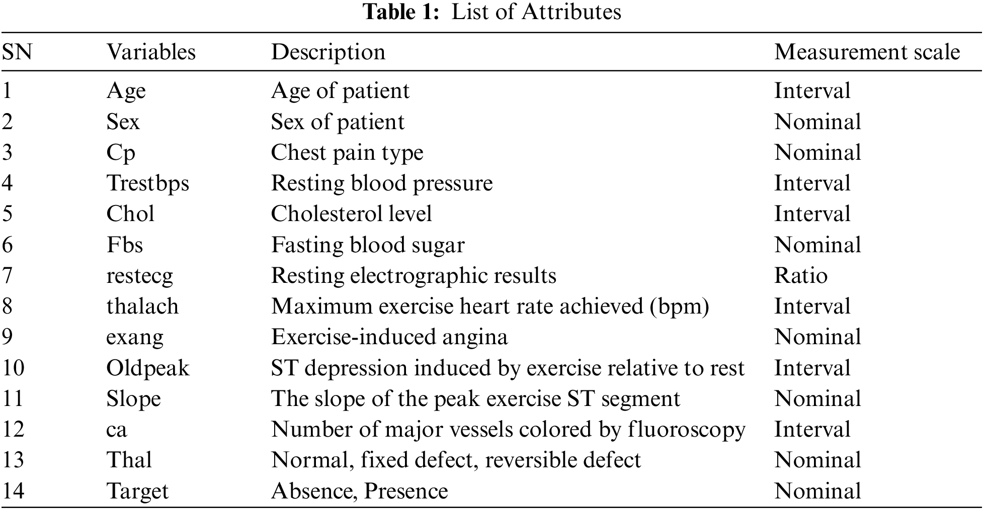
The heart is the major organ of the body which pumps blood and supplies it to the whole body. Life is dependent on the efficient working of the heart. If the heart cannot regulate blood to body parts, it may cause severe pain and mortality within minutes. Such disease needs to be treated on time [1]. Moreover, the number of heart diseases is increasing which causes it to be the number one cause of death worldwide [2]. According to a survey, the death rate due to heart disease (HD) in Pakistan has been reported as 15.36% and can raise to 23 million deaths by 2030 annually [3]. Early detection of such diseases can reduce the death rate. For this, there should be a predictive system that can assess the presence or absence of HD. The application of Machine Learning (ML) in the predictive analysis of diseases is very beneficial. It can play a vital role in providing the best algorithm which can classify whether a person is suffering from HD or not [4]. There is a numeral number of tests required to assess the presence of HD. Such data can be beneficial to finding hidden patterns by knowing one’s symptoms. Once symptoms are identified, they can be trained on ML models which can be helpful to identify one possesses HD or not [5]. Such a predictive system is very helpful for cardiologists in taking decisions quickly so that many people can be treated in a short time, thus saving thousands of life [6,7].
However, the main focus of the study is the empirical analysis of different ML techniques and finding the best technique amongst the prevailing techniques for the prediction of HD with higher accuracy and lesser amount of error rate. For evaluating existing techniques, this research focuses on Mean Absolute Error (MAE), Relative Absolute Error (RAE), Accuracy, Precision, Recall, and F-measure as assessment metrics to evaluate the employed techniques. The reason for using error rate is to find that how our prediction is wrong or what is the difference between actual and predicted outcomes. This is also in important factor to keep in consideration.
Hereinafter, Section 2 addresses the literature review, whereas Section 3 illustrates the study methodology. Section 4 went through the outcomes and how they were discussed. Finally, Section 5 summarizes the entire study’s findings.
The basic ML process comprises data collection, pre-processing, and applying a classifier on a dataset to diagnose diseases. The first step involves the preprocessing of raw data to form a clean dataset that can further be passed for the training phase, the second step involves the utilization of the classifier on the preprocessed dataset to evaluate the prediction accuracy of the classifier. Supervised learning involves the development of a model where labels are known. On the other side, the “unsupervised” research method is not pre-labeled.
Agreeing with information from the literature periodical, various data mining techniques are used for HDP with higher accuracy and fewer error rates [8]. Different types of studies have been conducted to target the prediction of HD, which includes the following related work: A framework for HDP named An Effective Classification Rule Technique for Heart Disease Prediction has been recommended by Vijayarani et al. [9]. The authors performed an experimental analysis of different classification rule techniques such as Decision Table (DTab), JRip, OneR, and Part on a dataset obtained from UCI which contains 14 features. Evaluation metrics are based on Accuracy and error rates namely MAE, RMSE, RAE, and RRSR. Post assessment, it is concluded the DTab performs better than other techniques with an accuracy of 73.6%.
Experimental analysis performed by Chaurasia et al. [10] on Naive Bayes (NB), J48 Decision Tree (DT), and Bagging algorithm on a dataset obtained from UCI which contains 11 features. Evaluation metrics are based on accuracy, precision, and recall matrix. Post assessment, it is concluded that the bagging algorithm has an accuracy of 85.03%. Comparative analysis performed by Venkatalakshmi et al. [11] on DT, NB on a dataset obtained from UCI which contains 14 features. Evaluation metrics are based on accuracy. Post assessment, it is concluded that NB with 85.03% outperforms other techniques. Masethe et al. [12] perform an empirical study on J48, Bayes Net, NB, Simple Cart (SC), and Reduced Error Pruning Tree (REPTREE) on a dataset obtained from UCI which contains 14 features. Evaluation metrics are based on accuracy. Post assessment, it is concluded that the prediction accuracy of J48 is 99%.
Dai et al. [13] perform experimental analysis on SVM, AdaBoost, Logistic Regression (LR), and NB on the dataset is obtained through clinical data. Evaluation metrics are based on accuracy. After the assessment, it is concluded that the prediction accuracy of AdaBoost is 82%. Abdar et al. [14] propose the C5.0 DT framework for HDP through comparative analysis on C5.0, SVM, K-nearest neighbor (KNN), and Artificial Neural Network (ANN). The dataset was obtained from UCI which contains 14 features. Evaluation metrics are based on accuracy. Post assessment, it is concluded that C5.0 has the greatest accuracy 93%. Umair Shafique, Fiaz Majeed, Haseeb Qaiser, and Irfan Ul Shafique et al. [15] perform a comparison among ML algorithms like J48, ANN, and NB on a dataset obtained from UCI which contains 14 features. Evaluation metrics are based on accuracy and time. After evaluating the results, it is concluded that NB outperforms other techniques with 82.9% and J-48 has an accuracy of 77.2%.
An intelligent technique for HDP proposed by Dbritto et al. [16] through comparative analysis among algorithms like NB, DT, KNN, and SVM on different datasets obtained from Cleveland, Hungary, Switzerland, long beach, and Stat log. Accuracy is used as an evaluation metric and concluded SVM better than other techniques with 80%.
An operational framework for HDP named Identification of heart failure by using unstructured data of cardiac patients proposed by Saqlain et al. [17] through comparative analysis on algorithms like LR, ANN, SVM, random forest (RF), DT, and NB. The comparative analysis was performed on a dataset obtained from the Armed Forces Institute of Cardiology (AFIC). Evaluation metrics are based on accuracy, precision, recall, and concluded NB performed best, with a predictive accuracy of 86%. For improving the predictive accuracy of the classifier, Weng et al. [18] perform a comparison among algorithms like RF, LR, gradient boosting (GB), and ANN. The different datasets were obtained from clinical data of 378,256 patients. Evaluation metrics are based on Area under the ROC Curve (AUC) and concluded ANN performed best, with predictive accuracy improving by 3.6%. Keerthana et al. [19] perform a comparison among algorithms like RF, DT, and NB. perform a comparison among algorithms like NB, DT, and RF. The dataset was obtained from UCI which contains 14 features. Evaluation metrics are based on accuracy, precision, and recall and concluded NB better performance than other techniques. To evaluate algorithms’ performance, Rairikar et al. [20] perform a comparison among algorithms like RF, DT, and NB on a dataset obtained from UCI datasets 14 attributes having 270 instances. Evaluation metrics are based on precision, recall, F-measure, ROC, PRC curve, and concluded RF better performance than other techniques with 75%.
Kumar et al. [21] perform a comparison among algorithms like J48, LMT, RF, NB, KNN, and SVM. The dataset was obtained from UCI which contains 14 features. Evaluation metrics are based on accuracy and time and concluded J48 has better performance than other techniques with 56.76% accuracy. An intelligent algorithm recommended by Hasan et al. [22] named Comparative Analysis of Classification Approaches for Heart Disease Prediction through comparison among algorithms like KNN, DT (ID3), NB, LR, and RF. The dataset obtained from UCI datasets 14 has 303 instances attributes. Evaluation metrics are based on accuracy, ROC curve, precision, recall, sensitivity, specificity, and F1-score, and concluded that LR performs better than other techniques 92.76%. Ramalingam et al. [23] perform an empirical study on algorithms like SVM, KNN, NB, DT, RF, and ensemble models The dataset was obtained from UCI datasets. Evaluation metrics are based on accuracy and concluded SVM is better than other techniques with an accuracy of 92.1%. To evaluate the performance of hybrid algorithms, Gultepe et al. [24] perform comparisons among meta algorithms like ensembling J48, ensembling NB on a dataset obtained from the UCI dataset having 14 attributes, and 303 instances. Evaluation metrics are based on accuracy, and concluded ensembling J48 better than other techniques with an accuracy of 81.31%.
A model has been developed to support decision-making in HD prognosis based on data mining techniques propose by Makumba et al. [25] on algorithms like DT, NB, and KNN using Waikato Environment for Knowledge Analysis application programming interface (WEKA API). Data for the proposed model has been accessed from UCI having 14 attributes. Evaluation metrics are based on accuracy. To assess the performance of an algorithm like J48 and NB for prognosis and identification of heart disease, Mohamed et al. [26] recommend NB. The comparative analysis was performed on the dataset obtained from the UCI dataset having 14 attributes and 303 instances. Results show NB is superior to others with an accuracy of 83%. KARLIK [27] evaluate classification algorithms like RF, SVM, LR, GB with receiver operating characteristic (ROC) curve for identification and prediction of a congestive problem. The dataset obtained from the UCI dataset has 14 attributes and 303 instances. Results show LR is superior to others with an accuracy of 87%. A bootstrap aggregation method proposed by Motarwar et al. [28] for HDP through a comparative analysis of RF, NB, SVM, Hoeffding Tree (HT), and Logistic Model Tree (LMT). The dataset obtained from the UCI dataset has 14 attributes and 303 instances. Evaluation metrics are based on accuracy and concluded RF better than other techniques with 95.08%.
Ware et al. [29] perform an empirical study on SVM, RF, KNN, DT, NB, and LR techniques to detect heart disease. The dataset obtained from the UCI dataset has 14 attributes and 303 instances. Evaluation metrics are based on accuracy measure, precision, and recall, and concluded SVM better than other techniques with 89.34%. To assess the performance of the algorithm in terms of higher accuracy proposed by Barik et al. [30] through comparative analysis on NB, DT, LR, and RF. The dataset obtained from the UCI dataset has 14 attributes and 303 instances. Evaluation metrics are based on accuracy, f measure, precision, and recall, and concluded RF better than other techniques with 90.16% accuracy.
The detailed methodology begins with a collection of two different HDDs, one is the UCI dataset and the other is the Kaggle dataset. Post collections of the dataset, classification techniques are applied to the dataset to achieve better accuracy and lower error rate. For this, techniques including J48, NB, LR, SC, Bagging, DS, AdaBoost, ANN, REPT, and SVM are first trained using 10 fold-cross validation (CV) on the dataset, and then the prediction is performed by each technique. Post predictions, analysis of comparisons were performed among all mentioned techniques to check which technique has higher accuracy and lower error rate. The overall methodology for HDP is shown in Fig. 1.

Figure 1: Research methodology
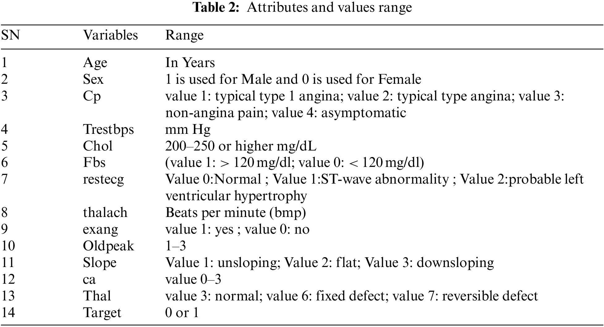
The ML classification techniques are employed on datasets taken from UCI and Kaggle repositories. The selection of these datasets is based on the waste use of these datasets in the previous research studies. These datasets are recommended by various researchers as standards for research analysis [29,31,32]. The dataset taken from the UCI repository contains 303 instances with 14 features1, and the dataset taken from the Kaggle ML repository contains 1025 instances and 14 attributes. Both the datasets have same attributes in which there are 13 independent features which include age of patient in years which is an interval value, gender of patient which is nominal, chest pain type whether it is angina, non-angina or asymptomatic and it is measured as nominal, blood pressure which is measured in interval scale and it has range of values between 90 to 250, Cholesterol level between 200–250 or higher and measured in interval scale, Blood sugar level which is measured in nominal scale and has value higher or lesser than 120, maximum cardiac rate achieved, Maximum exercise cardiac rate achieved and measured interval scale, Exercise induced angina which is measured in nominal scale and has values 0 or 1, Depression induced by angina which has range of values 1 to 3 and measured in interval scale, Slope of peak exercise which has range of values namely un-slopping, flat, down slopping, Number of vessels colored by fluoroscopy and range of values are between 0 to 3 and measured in interval scale, Thal which has three values namely normal, fixed defect, reversible defect and one dependent feature namely Target which has value yes or no and measured in nominal scale. The list of attributes and range for both the datasets are listed in Tabs. 1 and 2 respectively.
3.2 Dataset Splitting Using K-Fold Cross-Validation
To assess the performance of a classifier, the 10-fold cross-validation is applied. The 10-fold cross-validation is a technique that divides data records into 10 portions of equivalent sizes; one portion is utilized for validation set while others are used for training. This process continues until each portion has been utilized for validation. It is a standard technique used for assessment [33].
To determine techniques with higher accuracy and lower error rates, ten classification techniques including J48, NB, LR, SC, Bagging, DS, AdaBoost, ANN, REPT, and SVM have been used for comparisons. The subsection contains a brief detail of each employed technique.
The J48 algorithm grows the initial tree using the technique of divide and conquers. The root node is the attribute that has the highest gain ratio. To enhance accuracy, this technique uses pessimistic pruning to eliminate unnecessary branches in the tree. To treat continuous attributes, the algorithm segregates values into two divisions. The tree is pruned to avoid overfitting and can be seen in Eq. (1) and Eq. (2) [34].
where c is the number of classes, Pi is the proportion of S belonging to class ‘i’ [34].
where A is a set of all possible values, Sv is the subset of S for which function A has value v, S corresponds to entropy of the original collection, and the predicted value of entropy.
A basic yet very powerful solution is based on combining some weak classifiers into a strong classifier. Weak (or basic)” means poor performance and accuracy classifier is relatively low. It is especially for classification problems. It performs selecting the training set for each new classifier. A random subset of the overall training set will be equipped for every weak classifier. If each classifier has been equipped, the weight of the classifier is determined based on its accuracy. Mathematically, can be calculated as in Eq. (3) More accurate classifiers get more weight [35].
The final classifier is composed of weak classifiers ‘T’, “H t (x)” is the output of the low classifier ‘t’, “alpha t” is the weight added by AdaBoost to the classifier ‘t’. The final output is therefore just a linear combination of all the weak classifiers and the final judgment is taken simply by looking at the sign of this sum [35].
3.3.3 Reduced Error Pruning Tree
REPT is a quick decision tree. It follows the rationale for the regression tree and produces several trees in different iterations. Post, it selects the best one from all trees produced. The metric used in pruning the tree is the mean square error on tree predictions. It constructs a decision/regression tree using information gain as the criteria for separation, and prunes it using reduced pruning of errors and helps in reducing the variance. This sort values just once for numerical attributes. Missing values are addressed using the approach used by C4.5 for utilizing fractional instances [36]. This can be done via Eq. (4).
where A is a set of all possible values, Sv is the subset of S for which function A has value v, S corresponds to entropy of the original collection, and the predicted value of entropy.
3.3.4 Artificial Neural Network
A neural network is an ML built on a human neuron model. This algorithm was designed to simulate the human brain neurons. It involves several related processing units working together to process information. This is composed of several associated nodes or neurons, and one node’s output is another’s an entry. Every node receives several inputs but only one value is generated. A commonly used form of ANN, the Multi-Layer Perceptron (MLP) consists of an input layer that reflects the raw input that is allowed to flow through the network., hidden layers that identify the operation of each hidden object, and an output layer which depends on the operation of the hidden units and the weights between the hidden units and the output units. The important parts include the synapses, defined by their weight values, the summing junction (integrator), and the activation mechanism [37]. The output of the neuron k can be mathematically represented by a simple as Eq. (5):
where the input signals are j = 1, m, j = 1, m, are the synaptic weights of neuron k, is the net entry to the activation function, is the neuron bias, f (⋅) is the activation feature, and is the display. The activation function determines the contribution of the neuron k in addition to its network data [37].
SVM is a supervised algorithm for ML that can be used for classification or regression problems. The goal of the support vector machine algorithm is to find a hyperplane in an N-dimensional space where n is the number of features that classify the data points distinctly. Hyperplanes are boundaries for decision-making and help to distinguish data points. Support vectors are data points relative to the hyperplane, which influence the hyperplane’s position and orientation, and can be calculated as Eq. (6). The loss function which helps to optimize the margin is hinge loss [38].
where w, b is the hyperplane parameters and x is the variable(s) of the input. When
Bagging is used to enhance the accuracy and symmetry of ML techniques used in statistical regression and classification. It also helps in reducing variance and avoiding overfitting. Provide work for bagging on classifiers, particularly on decision trees, neural networks improve the precision of classification. Bagging plays a crucial role in the field of HD diagnosis [39].
LR algorithm is a regression and classification method for examining the dataset in which it contains one or more independent variables that conclude an outcome [40]. It is based on the Eq. (7):
In the training phase, coefficients of instances x1,x2,x3,… xn will be b0,b1,..bn. The coefficients are updated and estimated by stochastic gradient descent.
All the coefficients are 0 initially where l is the learning rate, x is the biased input for b0, which is always 1. The process of updating continues until the correct prediction is made at the training stage [40].
Bayesian Theorem delivers the foundation of NB. In this, singular parameters subsidize autonomously to the prospect as shown in Eq. (8) [38].
For example, the fruit is an apple that gives individualistically to the likelihood of apple, even though somewhat conceivable correlations between the roundness, color, and diameter features for classification. For classifying spatial datasets, the NB algorithm is desirable. This method achieves conditional independence. An attribute value is independent of other attributes to estimate conditional independence. So that it proves fruitful for investigating and getting information as in Eq. (9) [41].
SC is a classification technique that generates a binary decision tree. Because the output is a binary tree, it generates only two children. Attribute splitting is performed by the highest entropy. It uses a CV or a large number of the test sample to choose the best tree from a series of the tree which is considered as pruning process. The rationale behind the Simple Cart algorithm is a greedy algorithm in which the locally best feature is selected at each stage. The full process, it is computationally costly. In the implementation process, the dataset is divided into two groups that are unique concerning the outcome. This process continues until the small size subgroup reached [42]. The equations are Eq. (10), Eq. (11), and Eq. (12):
A DS is a learning model that consists of one decision tree. It has one internal node which connects to leaves immediately. For prediction, it uses a single input attribute. It is also known as 1-rules. There are variations possible depending on the type of input attribute. For binary and nominal type attributes, two leaves are possible. For numeric attributes, some values are selected and the stump contains two leaves such as below and above threshold [43].
3.4 Performance Assessment Criteria
Model assessment is the essential goal of any research work. It is important to evaluate with some standard evaluation measures/models. For evaluation of algorithms to achieve higher accuracy and lower error, assessment metrics involved namely MAE [44], RAE [45], accuracy [46], precision, recall [47], F-measure [48].
MAE can be determined by compelling the difference of incessant variables, for example, foreseen and witnessed values, final time against initial time. It can be calculated as Eq. (13):
Tentative or probing values are the two variables on which relative absolute error relies on. To measure the relative RAE, these two criteria must be recognized. RAE is obtained by the ratio of absolute error and the experimental value. Percentage or fraction is used to indicate relative absolute error because it has no units. Eq. (14) is used to find the value of RAE.
where
The numerator is equivalent to 0 for a good suit, and Ei = 0.
Accuracy is one criterion for assessing models of classification. Informally, accuracy is the proportion of our model’s observations that was accurate. Accuracy can be find using Eq. (16):
It is the ratio of optimistic successfully expected observations to predicted positive all-out observations. It can be calculated as Eq. (17):
A recall is the percentage of exactly expected optimistic findings to other actual class findings – yes. It can be calculated as Eq. (18)
It is the weighted average of Precision and Recall. This ranking takes into account all false negatives and false positives in certain lines. Instinctively it is not as straightforward as precision, however, F1-Measure is normally more helpful than accuracy, particularly if you have a lopsided class distribution. To find F-measure the Eq. (19) will be used:
This section presents the experimental results of SC and SVM with a comparison to employed techniques. Firstly, the results of employed models are discussed and then the results of SC and SVM are presented. The results are taken using two different HDDs. The results are evaluated using MAE, RAE, accuracy, precision, recall, and f-measure as evaluation metrics.
This section presents outcomes obtained through the analysis of classification algorithms. These models are evaluated on two different datasets using six evaluation metrics. Ten classifiers including J48, NB, LR, SC, Bagging, DS, AdaBoost, ANN, REPT, and SVM were tested on HDDs including the UCI dataset and Kaggle dataset with 10 fold CV on evaluation metrics which include RAE, MAE, correctly and incorrectly instances, accuracy, precision, recall, and f-measure for analyzing which algorithm works best in predicting HD.
4.1.1 Experimental Results Scenario 1 (UCI Dataset)
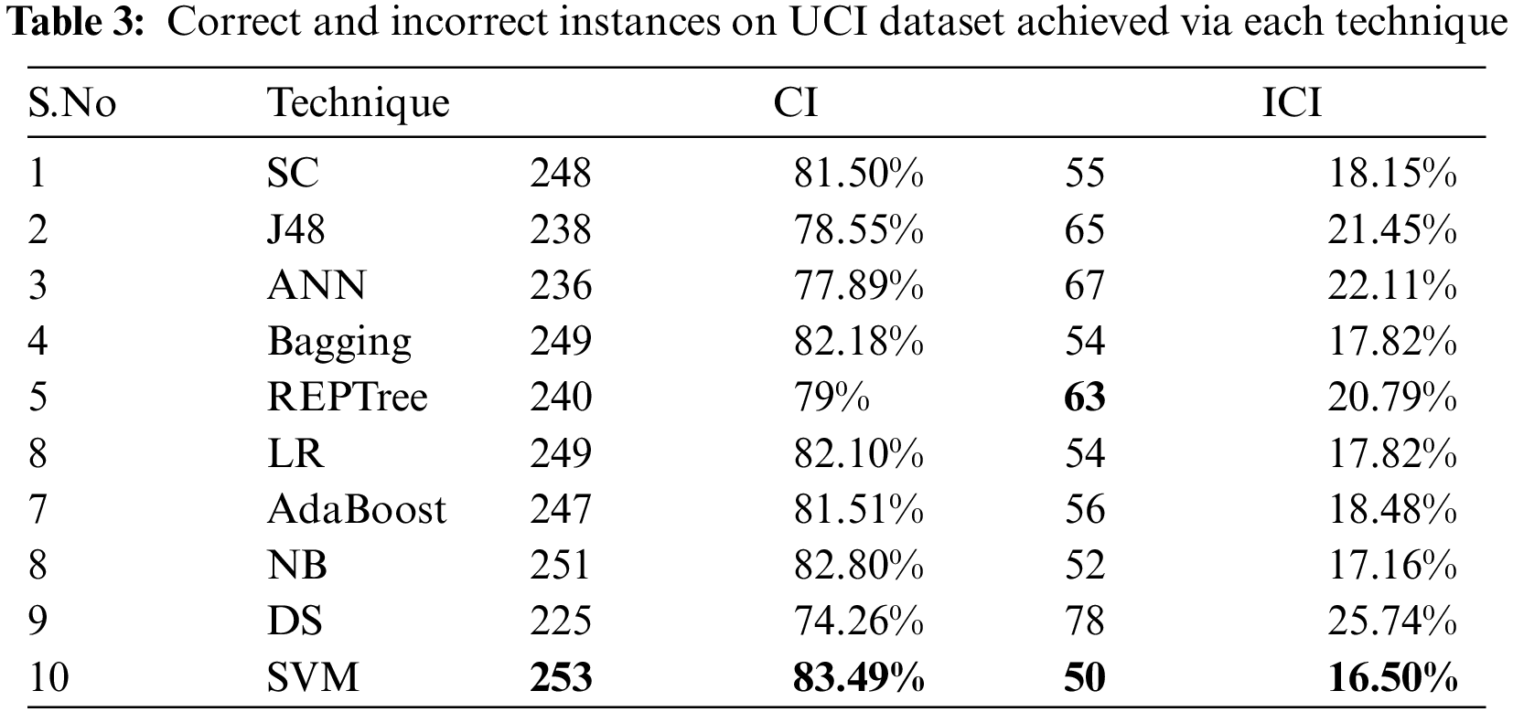
Tab. 3 shows the correct classified instances (CCI) and incorrect classified instances (ICI) by employed algorithms on the UCI dataset. Thus it shows how many instances of the dataset have been performed correctly or incorrectly by each algorithm. It clearly shows that SVM with 253 correct and 50 incorrect instances outperforms J48, NB, LR, SC, Bagging, DS, AdaBoost, ANN, and REPT.
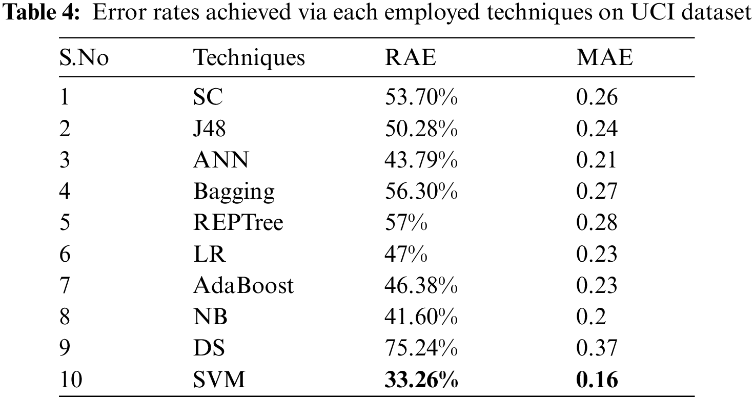
Tab. 4 shows the error rates which include RAE and MAE for the employed techniques. By analyzing, SVM produces better results for error rates namely RAE as 33.26% value, MAE as 0.16 value.
As the SVM algorithm performed better on UCI dataset than the other techniques with lower error rates, Tab. 5 presents the difference between error rates among SVM and other employed classifiers.

For evaluating algorithms, there ought to be some metric to predict the correctness of the algorithm. For this, accuracy is highly important to check how correctly it is performing. Tab. 6 represents the analysis of precision, recall, F-measure, and accuracy achieved via each classifier. These outcomes show the better performance of the SVM algorithm as compared to other employed algorithms. Fig. 2 represents the analysis achieved via precision, recall, and F-measure while Fig. 3 presents the accuracy details.
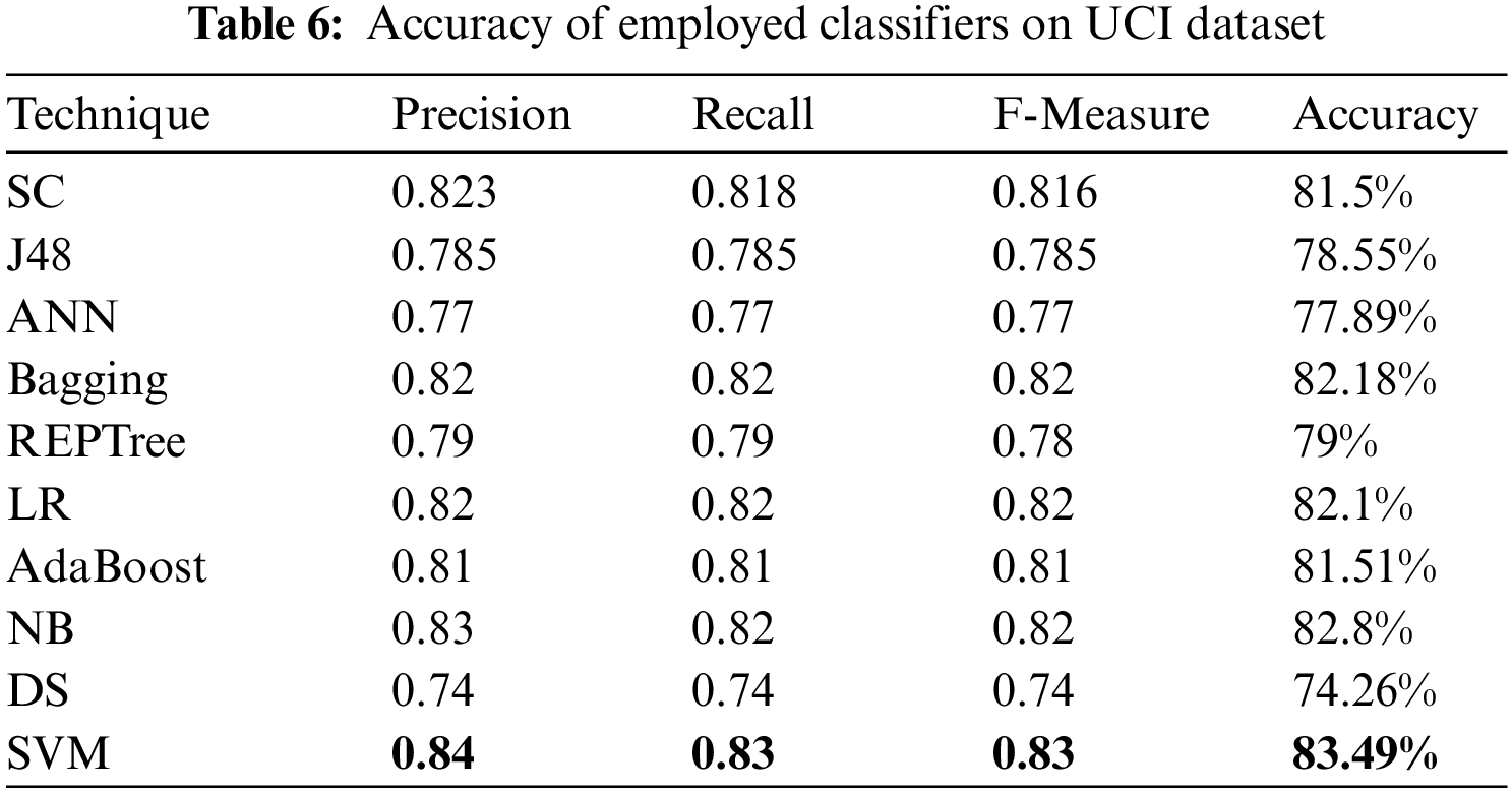

Figure 2: Precision, recall and F-measure analysis on UCI dataset

Figure 3: Accuracy achieved vie each classifier on UCI dataset
When comparing the SVM with the employed techniques on the UCI dataset, the difference of accuracy between SVM and employed techniques is given in Fig. 4. The percentage difference is calculated through Eq. (20) as follows:
Here, v1 represents the value of SVM while v2 represents the value of other techniques compared with SVM. While in Fig. 7, v1 presents the value of SC.

Figure 4: Accuracy percentage difference between SVM and other employed classifiers on UCI dataset
4.1.2 Experimental Results Scenario 2 (Kaggle Dataset)
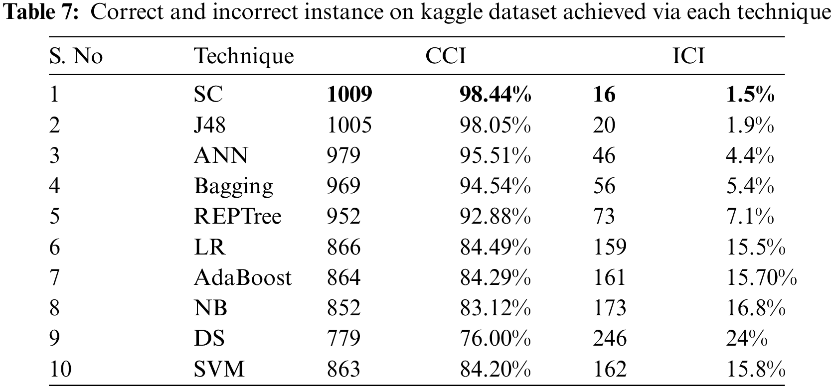
Tab. 7 shows the CCI and ICI by employing algorithms on the Kaggle dataset. Thus it shows how many instances of the dataset have been performed correctly or incorrectly by each algorithm. It clearly shows that SC with 1009 correct and 16 incorrect instances outperforms J48, NB, LR, SC, Bagging, DS, AdaBoost, ANN, and REPT as shown in Tab. 7.
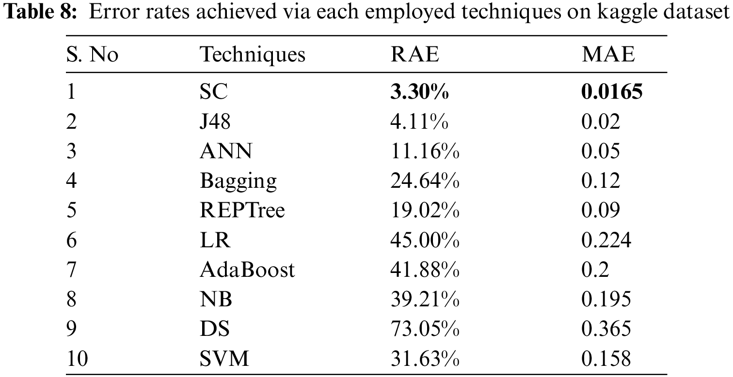
Tab. 8 shows the error rates which include RAE and MAE for the employed techniques on the Kaggle dataset. By examining Tab. 8, it is known that SC has lesser error rates than compared techniques with 3.30% as RAE value and 0.0165 as MAE value.
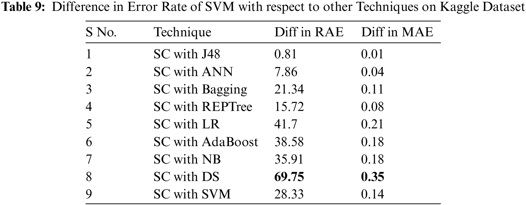
As the SC algorithm performed better on Kaggle dataset than the other techniques with lower error rates, Tab. 9 presents the difference between error rates among SC and other employed classifiers.
For evaluating algorithms, there ought to be some metric to predict the correctness of the algorithm. For this, accuracy is highly important to check how correctly it is performing. Tab. 10 represents the analysis of precision, recall, and F-measure achieved via each classifier. These outcomes show the better performance of the SC algorithm as compared to other employed algorithms. Fig. 5 represents the analysis achieved via precision, recall, and F-measure while Fig. 6 presents the accuracy details.
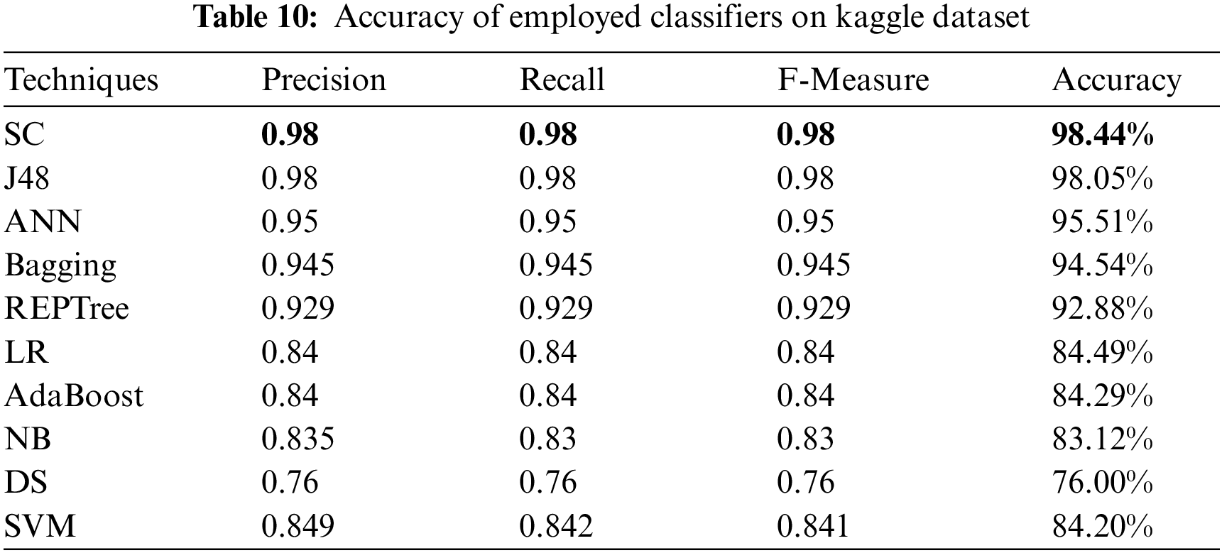

Figure 5: Precision, recall and F-measure analysis on kaggle dataset

Figure 6: Accuracy achieved vie each classifier
When comparing SC with the employed techniques on the Kaggle dataset, the difference of accuracy between SC and employed techniques is given in Fig. 7.

Figure 7: Accuracy percentage difference between SC and other employed classifiers
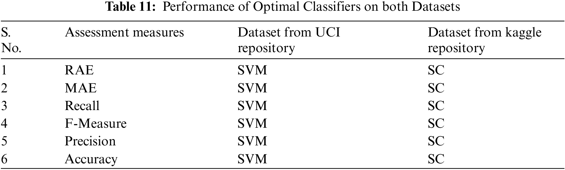
This study aims to perform an empirical analysis of ten different ML classification algorithms on two different HDDs taken from Kaggle and UCI repositories. On both datasets, results, after the assessment is a heterogeneous due to each dataset, containing a different amount of instances dataset according to attributes and most important, different amounts (percentage) of effective and non-effective patient records. Tab. 11 shows the better performance of better classifiers on both datasets concerning each assessment measure. These analyses illustrate that in terms of reducing the error rate on both datasets and maximizing accuracy. However, on the UCI dataset, SVM produces better results for precision, recall, f-measure, accuracy, and error rates namely RAE, MAE. On the other side, the dataset is taken from the Kaggle repository, SC performs better in terms of increasing accuracy, precision, recall, and F-measure with reducing error rates namely MAE and RAE. The results are different on each dataset due the number of instances and variations in the values of records.
This work may have certain limitations that are addressed as challenges to authenticity. These risks include changing the dataset, increasing or decreasing the number of occurrences in the dataset, which may alter the results of this work. It is also possible that using new procedures or assessment criteria would disrupt the present analysis. Furthermore, changing the testing and training criteria will result in a change in the existing outcomes.
The performance of SVM is better on UCI dataset that is due the dataset that applied to algorithms was taken from the UCI repository which contains 303 instances with 14 attributes. The dataset is pre-processed which means the SVM has linearly separated the data causing the margin to be maximized on the UCI dataset. To get the maximum margin to best fit our data, we have used a polynomial kernel function that can plot data in high dimensional. Moreover, the parameters are tuned due to which SVM has better performance on the UCI dataset. According to over data, it is also known about SVM that when there is a clear margin of distinction between classes, SVM performs rather well. In high-dimensional spaces, SVM is more effective, and is effective when the number of dimensions exceeds the number of samples. It also performs and generalizes effectively on data that is not from a sample. Another reason to use SVM is that making minor changes to the derived feature data does not influence the previously predicted results. It is rapidly converging, and as previously indicated in the article Kernel Functionality, in general, the Polynomial kernel appears to be a better factor in terms of SVM [49,50]. However, the performance of SC is better on the Kaggle dataset because of the dataset used to train the algorithms was obtained from the Kaggle repository, which comprises 1025 instances with 14 characteristics. The dataset has been pre-processed, which means SC generates a binary DT by repeatedly separating a node into two child nodes, beginning with the root node, which holds the whole learning sample. We adjusted the pruning option to true for greater performance, and cross-validation up to 5 folds fit more precisely, making the decision tree an excellent learner. Furthermore, because the number of instances in the Kaggle dataset is greater than the number of instances in the UCI dataset, some other reasons for the SC’s superior performance include the fact that the SC focuses on detecting interactions and signal discontinuities and automatically identifies significant factors. It may employ any mix of continuous/discrete variables and is insensitive to predictor monotone transformations. To more precisely quantify the goodness of fit, it combines testing using a test data set with cross-validation [51,52].
It is observed from the literature that several kinds of research developed techniques for HDP but it is still a challenging task in terms of increasing accuracy and decreasing error rate. The focus of this research is to improve the accuracy rate of HDP in terms of reducing the error rate of the evaluation metric using two algorithms i.e., SVM for a UCI dataset and SC for Kaggle datasets. The datasets from UCI and Kaggle data repositories were selected and MAE, RAE, accuracy, precision, recall, and f-measure are used as evaluation metrics. The results taken from the proposed models are compared with the results of the employed techniques used for comparative analysis. The eventual goal of this research is to reduce the error rate and maximize accuracy for techniques used in research for HDP. Improvement in results can be performed by using the latest algorithm with the latest datasets can also be applied to improve the accuracy results of HDP and merging the strength of SVM, SC to enhance the proficiency and performance which is known as hybridization. In the future, we can combine SVM with SC to design an ensemble model that may produce better performance on any relevant dataset. Moreover, SVM or SC can also be hybridized with any other searching optimization techniques to find a better solution for aforementioned problem.
Acknowledgement: Authors would like to acknowledge the support of the Deputy for Research and Innovation- Ministry of Education, Kingdom of Saudi Arabia for this research through a grant (NU/IFC/ENT/01/014) under the institutional Funding Committee at Najran University, Kingdom of Saudi Arabia.
Funding Statement: Authors would like to acknowledge the support of the Deputy for Research and Innovation- Ministry of Education, Kingdom of Saudi Arabia for this research at Najran University, Kingdom of Saudi Arabia.
Conflicts of Interest: The authors declare that they have no conflicts of interest to report regarding the present study.
1https://archive.ics.uci.edu/ml/datasets/Heart+Disease
References
1. D. Chicco and G. Jurman, “Machine learning can predict survival of patients with heart failure from serum creatinine and ejection fraction alone,” BMC Medical Informatics and Decision Making, vol. 20, no. 1, pp. 1–16, 2020. [Google Scholar]
2. T. A. Gaziano, A. Bitton, S. Anand, S. Abrahams-gessel and A. Murphy, “Growing epidemic of coronary heart disease in low- and middle-income countries,” Current Problems in Cardiology, vol. 35, no. 2, pp. 72–115, 2010. [Google Scholar]
3. A. G. Shaper, “Risk factors for ischaemic heart disease,” Health Trends, vol. 19, no. 2, pp. 3–8, 1987. [Google Scholar]
4. S. Uddin, A. Khan, M. E. Hossain and M. A. Moni, “Comparing different supervised machine learning algorithms for disease prediction,” BMC Medical Informatics and Decision Making, vol. 19, no. 1, pp. 1–16, 2019. [Google Scholar]
5. A. U. Haq, J. Li, M. H. Memon, M. Hunain Memon, J. Khan et al., “Heart disease prediction system using model of machine learning and sequential backward selection algorithm for features selection,” in 5th Int. Conf. for Convergence in Technology, Pune, India, pp. 1–4, 2019. [Google Scholar]
6. A. U. Haq, J. P. Li, M. H. Memon, S. Nazir, R. Sun et al., “A hybrid intelligent system framework for the prediction of heart disease using machine learning algorithms,” Mobile Information Systems, vol. 1, no. 1, pp. 25–35, 2018. [Google Scholar]
7. K. M. Aamir, M. Ramzan, S. Skinadar, H. U. Khan, U. Tariq et al., “Automatic heart disease detection by classification of ventricular arrhythmias on ecg using machine learning,” CMC-Computers Materials & Continua, vol. 71, no. 1, pp. 17–33, 2022. [Google Scholar]
8. V. A. Tatsis, C. Tjortjis and P. Tzirakis, “Evaluating data mining algorithms using molecular dynamics trajectories,” International Journal of Data Mining and Bioinformatics, vol. 8, no. 2, pp. 169–187, 2013. [Google Scholar]
9. S. Vijayarani and S. Sudha, “An effective classification rule technique for heart disease prediction,” International Journal of Engineering Associates, vol. 1, no. 4, pp. 81–85, 2013. [Google Scholar]
10. V. Chaurasia and S. Pal, “Data mining approach to detect heart diseases,” International Journal of Advanced Computer Science and Information Technology, vol. 2, no. 4, pp. 56–66, 2014. [Google Scholar]
11. B. Venkatalakshmi and M. V. Shivsankar, “Heart disease diagnosis using predictive datamining,” International Journal of Innovative Research in Science, Engineering and Technology, vol. 3, no. 3, pp. 1873–1877, 2014. [Google Scholar]
12. H. D. Masethe and M. A. Masethe, “Prediction of heart disease using classification algorithms,” Proceedings of the World Congress on Engineering and Computer Science, vol. 2, no. 1, pp. 25–29. 2014. [Google Scholar]
13. W. Dai, T. S. Brisimi, W. G. Adams, T. Mela, V. Saligrama et al., “Prediction of hospitalization due to heart diseases by supervised learning methods,” Journal of Medical Informatics, vol. 84, no. 3, pp. 189–197, 2015. [Google Scholar]
14. M. Abdar, S. R. N. Kalhori, T. Sutikno, I. M. I. Subroto and G. Arji, “Comparing performance of data mining algorithms in prediction heart diseses,” International Journal of Electrical & Computer Engineering, vol. 5, no. 6, pp. 1569–1576, 2015. [Google Scholar]
15. U. Shafique and L. Campus, “Data mining in healthcare for heart diseases,” International Journal of Innovation and Applied Studies, vol. 10, no. 4, pp. 1312–1322, 2015. [Google Scholar]
16. R. Dbritto, A. Srinivasaraghavan and V. Joseph, “Comparative analysis of accuracy on heart disease prediction using classification methods,” International Joutnal of Applied Information System, vol. 11, no. 2, pp. 22–25, 2016. [Google Scholar]
17. M. Saqlain, W. Hussain, N. A. Saqib and M. A. Khan, “Identification of heart failure by using unstructured data of cardiac patients,” in 45th Int. Conf. on Parallel Processing Workshops, Philadelphia, PA, USA, pp. 426–431, 2016. [Google Scholar]
18. S. F. Weng, J. Reps, J. Kai, J. M. Garibaldi and N. Qureshi, “Can machine-learning improve cardiovascular,” PloS one, vol. 51, no. 3, pp. e0174944–e01749–55, 2015. [Google Scholar]
19. T. K. Keerthana, “Heart disease prediction system using data mining method,” International Journal of Engineering Trends and Technology, vol. 47, no. 6, pp. 361–363, 2017. [Google Scholar]
20. A. Rairikar, V. Kulkarni, V. Sabale, H. Kale and A. Lamgunde, “Heart disease prediction using data mining techniques,”in Int. Conf. on Intelligent Computing and Control, I2C2, Coimbatore, India, pp. 1–8, 2018. [Google Scholar]
21. M. N. Kumar, K. V. S. Koushik and K. Deepak, “Prediction of heart diseases using data mining and machine learning algorithms and tools,” International Journal of Scientific Research in Computer Science, Engineering and Information Technology, vol. 3, no. 3, pp. 887–898, 2018. [Google Scholar]
22. S. M. M. Hasan, M. A. Mamun, M. P. Uddin and M. A. Hossain, “Comparative analysis of classification approaches for heart disease prediction,” in Int. Conf. on Computer, Communication, Chemical, Material and Electronic Engineering, Rajshahi, Bangladesh, pp. 1–4, 2018. [Google Scholar]
23. V. V. Ramalingam, A. Dandapath and M. Karthik Raja, “Heart disease prediction using machine learning techniques : A survey,” International Journal of Engineering & Technology, vol. 7, no. 2.8, pp. 684–687, 2018. [Google Scholar]
24. Y. Gultepe and S. Rashed, “The use of data mining techniques in heart disease prediction,” International Journal of Computer Science and Mobile Computing, vol. 8, no. 4, pp. 136–141, 2019. [Google Scholar]
25. D. O. Makumba, W. Cheruiyot and K. Ogada, “A model for coronary heart disease prediction using data mining classification techniques,” Asian Journal of Research in Computer Science, vol. 3, no. 4, pp. 1–19, 2019. [Google Scholar]
26. T. S. Mohamed and M. H. Ali, “Heart diseases prediction using weka,” Journal of Baghdad College of Economic Sciences University, vol. 20, no. 58, pp. 395–404, 2019. [Google Scholar]
27. KARLIK, B, “Soft computing methods in bioinformatics: A comprehensive review,” Mathematical and Computational Applications, vol. 18, no. 3, pp. 176–197, 2013. [Google Scholar]
28. P. Motarwar, A. Duraphe, G. Suganya and M. Premalatha, “Cognitive approach for heart disease prediction using machine learning,” in Int. Conf. on Emerging Trends in Information Technology and Engineering, Vellore, India, pp. 1–5, 2020. [Google Scholar]
29. S. Ware, S. Rakesh and B. Choudhary, “Heart attack prediction by using machine learning techniques,” International Journal of Recent Technology and Engineering, vol. 8, no. 5, pp. 1577–1580, 2020. [Google Scholar]
30. S. Barik, S. Mohanty, D. Rout, S. Mohanty, A. K. Patra et al., “Heart disease prediction using machine learning techniques,” Advances in Electrical Control and Signal Systems, vol. 665, no. 4, pp. 879–888, 2020. [Google Scholar]
31. S. Manjunath, M. B. Sanjay Pande, B. N. Raveesh and G. K. Madhusudhan, “Brain tumor detection and classification using convolution neural network,” International Journal of Recent Technology and Engineering, vol. 8, no. 1, pp. 34–40, 2019. [Google Scholar]
32. B. Khan, R. Naseem, F. Muhammad, G. Abbas and S. Kim, “An empirical evaluation of machine learning techniques for chronic kidney disease prophecy,” IEEE Access, vol. 8, no. 1, pp. 55012–55022, 2020. [Google Scholar]
33. M. M. Ahsan and Z. Siddique, “Machine learning-based heart disease diagnosis: A systematic literature review,” Artificial Intelligence in Medicine, vol. 128, no. 1, pp. 102289, 2022. [Google Scholar]
34. S. Singaravelan, D. Murugan and S. Mayakrishnan, “Asian research consortium A study of data classification algorithms j48 and smo on different datasets,” Asian Journal of Research in Social Sciences and Humanities, vol. 6, no. 6, pp. 1276–1280, 2016. [Google Scholar]
35. Y. Cao, Q. G. Miao, J. C. Liu and L. Gao, “Advance and prospects of adaboost algorithm,” Acta Automatica Sinica, vol. 39, no. 6, pp. 745–758, 2013. [Google Scholar]
36. S. Kalmegh, “Analysis of WEKA data mining algorithm reptree, simple cart and randomtree for classification of Indian news,” International Journal of Innovative Science,” Engineering & Technology, vol. 2, no. 2, pp. 438–446, 2015. [Google Scholar]
37. M. I. Al-janabi, M. H. Qutqut and M. Hijjawi, “Machine learning classification techniques for heart disease prediction: A review.” International Journal of Engineering & Technology, vol. 7, no. 4, pp. 5373–5379, 2018. [Google Scholar]
38. M. Panaite, M. Dascalu and A. Johnson, “Bring it on ! challenges encountered while building a comprehensive tutoring system using readerbench," in Int. Conf. on Artificial Intelligence in Education, London, United Kingdom, pp. 409–419, 2018. [Google Scholar]
39. G. T. Prasanna Kumari, “A study of bagging and boosting approaches to develop meta-classifier,” Engineering Science and Technology: An International Journal, vol. 2, no. 5, pp. 2250–3498, 2012. [Google Scholar]
40. M. Korkmaz, S. Güney and Ş Yüksel YİĞÎTER, “The importance of logistic regression implementations in the turkish livestock sector and logistic regression implementations/fields,” Harran Tarım ve Gıda Bilimleri Dergisi, vol. 16, no. 2, pp. 25–36, 2012. [Google Scholar]
41. A. Thomas and A. K. Sujatha, “Comparative study of recommender systems,” in Int. Conf. on Circuit, Power and Computing Technologies, Nagercoil, India, pp. 1–6, 2016. [Google Scholar]
42. S. Kaur and H. Kaur, “Review of decision tree data mining algorithms: CART and C4.5,” International Journal of Advanced Research in Computer Science, vol. 8, no. 4, pp. 4–8, 2017. [Google Scholar]
43. N. K. Al-Salihy and T. Ibrikci, “Classifying breast cancer by using decision tree algorithms,”in 6th Int. Conf. on Software and Computer Applications, Bangkok, Thailand, pp. 144–148, 2017. [Google Scholar]
44. C. J. Willmott and K. Matsuura, “Advantages of the mean absolute error (MAE) over the root mean square error (RMSE) in assessing average model performance,” Climate Research, vol. 30, no. 1, pp. 79–82, 2005. [Google Scholar]
445. F. Collopy and J. Armstrong, “Error measures for generalizing about forecasting methods: Empirical comparisons,” International Journal of Forecasting, vol. 8, no. 1, pp. 69–80, 1992. [Google Scholar]
46. M. Sokolova, N. Japkowicz and S. Szpakowicz, “Beyond accuracy, F-score and ROC: A family of discriminant measures for performance evaluation,” in Australasian Joint Conf. on Artificial Intelligence, Hobart, Australia, pp. 24–29, 2006. [Google Scholar]
47. T. Saito and M. Rehmsmeier, “The precision-recall plot is more informative than the ROC plot when evaluating binary classifiers on imbalanced datasets,” PLoS One, vol. 10, no. 3, pp. 1–21, 2015. [Google Scholar]
48. J. De Weerdt, M. De Backer, J. Vanthienen and B. Baesens, “A robust F-measure for evaluating discovered process models,” in IEEE Symp. on Computational Intelligence and Data Mining, Paris, France, pp. 148–155, 2011. [Google Scholar]
49. G. Manogaran, R. Varatharajan and M. K. Priyan, “Hybrid recommendation system for heart disease diagnosis based on multiple kernel learning with adaptive neuro-fuzzy inference system,” Multimedia Tools and Applications, vol. 77, no. 4, pp. 4379–4399, 2018. [Google Scholar]
50. K. L. Chiew, C. L. Tan, K. S. Wong, K. S. C. Yong and W. K. Tiong, “A new hybrid ensemble feature selection framework for machine learning-based phishing detection system,” Information Sciences, vol. 484, no. 1, pp. 153–166, 2019. [Google Scholar]
51. R. Tishirani and T. Hastie, “Margin trees for high-dimensional classification,” Journal of Machine Learning Research, vol. 8, no. 1, pp. 637–652, 2007. [Google Scholar]
52. D. L. Miholca, G. Czibula and I. G. Czibula, “A novel approach for software defect prediction through hybridizing gradual relational association rules with artificial neural networks,” Information Sciences, vol. 441, no. 1, pp. 152–170, 2018. [Google Scholar]
 | This work is licensed under a Creative Commons Attribution 4.0 International License, which permits unrestricted use, distribution, and reproduction in any medium, provided the original work is properly cited. |