| Computer Modeling in Engineering & Sciences |
DOI: 10.32604/cmes.2021.012686
ARTICLE
Study on the Improvement of the Application of Complete Ensemble Empirical Mode Decomposition with Adaptive Noise in Hydrology Based on RBFNN Data Extension Technology
1School of Water Conservancy Engineering, Zhengzhou University, Zhengzhou, 450001, China
2Yellow River Institute for Ecological Protection & Regional Coordinated Development, Zhengzhou University, Zhengzhou, 450001, China
3North China University of Water Resources and Electric Power, Zhengzhou, 450046, China
4School of Civil Engineering and Environmental Sciences, University of Oklahoma, Norman, OK, 73019, USA
*Corresponding Author: Bin Sun. Email: sunbin@zzu.edu.cn
Received: 08 July 2020; Accepted: 14 October 2020
Abstract: The complex nonlinear and non-stationary features exhibited in hydrologic sequences make hydrological analysis and forecasting difficult. Currently, some hydrologists employ the complete ensemble empirical mode decomposition with adaptive noise (CEEMDAN) method, a new time-frequency analysis method based on the empirical mode decomposition (EMD) algorithm, to decompose non-stationary raw data in order to obtain relatively stationary components for further study. However, the endpoint effect in CEEMDAN is often neglected, which can lead to decomposition errors that reduce the accuracy of the research results. In this study, we processed an original runoff sequence using the radial basis function neural network (RBFNN) technique to obtain the extension sequence before utilizing CEEMDAN decomposition. Then, we compared the decomposition results of the original sequence, RBFNN extension sequence, and standard sequence to investigate the influence of the endpoint effect and RBFNN extension on the CEEMDAN method. The results indicated that the RBFNN extension technique effectively reduced the error of medium and low frequency components caused by the endpoint effect. At both ends of the components, the extension sequence more accurately reflected the true fluctuation characteristics and variation trends. These advances are of great significance to the subsequent study of hydrology. Therefore, the CEEMDAN method, combined with an appropriate extension of the original runoff series, can more precisely determine multi-time scale characteristics, and provide a credible basis for the analysis of hydrologic time series and hydrological forecasting.
Keywords: Complete ensemble empirical mode decomposition with adaptive noise; data extension; radial basis function neural network; multi-time scales; runoff
The variation of runoff has multiple time scale features [1–4]. The exploration of runoff fluctuation and the trends of each time scale are important to the understanding of the inherent laws of hydrological elements and making runoff predictions [5,6]. However, the runoff series exhibit complicated nonlinear and non-stationary characteristics, as they are affected by various factors including climate change, interactions between social and hydrologic systems, etc. This complexity makes multi-time scale analysis difficult [7–9]. Therefore, development of an effective method to extract accurate and reliable information from intricate hydrologic sequences is requisite.
Wavelet transformation [10,11] and empirical mode decomposition (EMD) [12,13] are common time-frequency analysis methods for processing non-stationary series [14]. In particular, EMD has become increasingly popular owing to its completeness, adaptability, and approximate orthogonality compared to the wavelet technique [15,16]. Nevertheless, mode mixing may reduce the decomposition accuracy in EMD [13]. To overcome this issue, Torres et al. [17] proposed a complete ensemble empirical mode decomposition with adaptive noise (CEEMDAN), an advanced version of the ensemble empirical mode decomposition (EEMD) [18]. This new method can more precisely decompose nonlinear series and distinguish the variation patterns of different time scales in complex data [19,20]. Recently, many hydrologists have applied the CEEMDAN method to hydrological time series analysis [21–23] and built runoff prediction models combined with the “decomposition–prediction–reconstruction” principle [6,24–27].
It is worth noting that the endpoint effect caused by the cubic spline interpolation used in the EMD method presents another problem in addition to mode mixing [13,28]. The CEEMDAN method retains the original EMD algorithm without improving the interpolation algorithm, and the endpoint effect can lead to distortion of the decomposition results. Hydrologists usually ignore this issue and directly use CEEMDAN to decompose raw data without inhibiting the boundary error in their studies [6,21,22,27]. Consequently, the fluctuation characteristics reflected by the decomposition results may not align with the actual situation in each time scale, thereby reducing the reliability of the multi-time scale analysis. Additionally, as input to the runoff prediction model, the accuracy of the decomposition results is crucial to the “decomposition–prediction–reconstruction” principle. If the input data deviate from the real situation, the prediction cannot achieve the optimal effect. Few hydrologic studies have focused on the influences of the endpoint effect on decomposition and subsequent prediction accuracy. This study investigates these impacts, as well as reduces the boundary error prior to the runoff time series analysis and forecasting, via data extension technology to improve the reliability of the results.
In previous studies analyzing the endpoint effect in EMD, many mitigating solutions utilizing data extension have been proposed, including such techniques as mirror extending [29], extreme point symmetrical extending [30], AR models [31], and ANN models [28,32]. Each of these approaches has demonstrated good performance in specific situations. Among them, the radial basis function neural network (RBFNN) extension technique, a type of ANN model, has become a common and a suitable method for processing sequences with nonlinear characteristics [33–35]. Therefore, we selected the RBFNN technique to lengthen the original runoff series in order to suppress the endpoint effect of the CEEMDAN method in this study.
The steps taken to evaluate the inclusion of the RBFNN extension technique are as follows. (1) Extend the original annual runoff sequence using the RBFNN extension method to get an extension sequence. Contrast the results with the standard sequence to understand the results of the extension. (2) Individually decompose the original sequence, extension sequence, and standard sequence via CEEMDAN. Using the standard sequence as the base criterion, analyze the visual graphs of the decomposition results and quantify the decomposition error of the original and extension sequences. (3) Study the influence of the existing boundary error in CEEMDAN on the hydrological time series analysis and forecasting and the improvement effect of the RBFNN extension method. (4) Discuss and summarize the results of the above comparative analysis.
2.1 Complete Ensemble Empirical Mode Decomposition with Adaptive Noise (CEEMDAN)
The CEEMDAN method can precisely decompose nonlinear and non-stationary time series into several layers of intrinsic mode function (IMF) components and one residue (Res) without mode mixing and reconstruction error [17,36,37]. The IMFs, stability, and quasi-periodicity of the CEEMDAN method increase layer by layer and reflect the fluctuation characteristics of the sequence in multiple time scales. In addition, the Res can be regarded as the trend of the entire series. Therefore, CEEMDAN is an efficient tool for hydrological time series analysis and forecasting.
The CEEMDAN algorithm is given by

where  is the series to be decomposed,
  is the EMD operator used to obtain the
  th mode, and
  is the local average operator used to produce a new series for further decomposition. The term
  (
( ) is a zero-mean unit-variance white Gaussian noise that is added to the original series to generate
  .
.  is the operator for the mean calculation. The parameter
  represents the level of added noise, where
  ,
,  , and
, and  , where
  is the additive noise representing the signal-to-noise ratio and can be controlled at each stage.
Step 1: According to  , the first residue by EMD decomposition is given by

Step 2: The first intrinsic mode is calculated as

Step 3: The local mean of  is considered an estimate of the second residue, which leads to the second IMF component given by

Step 4: For  , the kth residue is calculated as

Step 5: The kth intrinsic mode is calculated as

Step 6: The process is repeated from Step 4 for next value of k.
Steps 4 to 6 are repeated until the residual value satisfies one of the following conditions: (1) IMF component conditions are met, (2) the number of extrema is less than three, or (3) the residue can no longer be decomposed.
Ultimately, the final residue is satisfied by

where  is the maximum number of components. Thus, the original series,
  , can be reconstructed using the equation given by

The CEEMDAN method repeatedly uses  (i.e., the EMD algorithm) in the decomposition process, thus reducing the decomposition accuracy by the endpoint effect.
2.2 Radial Basis Function Neural Network (RBFNN) Extension
The RBFNN technique has been widely used to forecast nonlinear time series, as it has the advantages of simple topology, a fixed network structure, and fast and efficient learning [38–43].
The process of utilizing the RBFNN extension can be described as follows [32]:
For the original series  , where
  is the number of raw data, a learning sample matrix,
  , and corresponding target matrix,
  , are generated. They are primarily created according to a certain rule, where
  is the number of sample groups, and
  stand for the number of data points in each group of samples. In the MATLAB toolbox, the built-in newrbe function is used to design a standard radial basis network (input sample
  ) to train the network and select an appropriate parameter value for spread to obtain the optimal radial basis network. In the process of model building, the radial basis function was program default, the number of neurons in the input layer was selected between 5–30, the number of neurons in the output layer was 1, and the parameter of spread was selected near the default value of 1. If the number of neurons is 5, the training set is
  ,
,  ,
,  and the test set is
  . RBFNN models have been evaluated by repeated cross-validation.
Next, the RBFNN network is applied for data extension. The sample matrix,  , is determined at the boundary (such as the right boundary) of the original series
  . Then, the sample matrix is input into the trained RBF network to obtain extension data
  . Data point
  is taken as the endpoint of extended sequence
  and used to generate sample matrix
  . The process is then repeated as sample matrix
  is input into the network again to obtain extension data
  . Ultimately, an extension series of suitable length,
  , where
  is the number of continuation points on the right, is obtained. In a similar fashion, the raw data can be extended on the other end to obtain the extension sequence
  , where
  represents the continuation points on the right, and
  is the number of points.
The prediction accuracy will decline invariably along with an increase in predictive time length. Extension data outside of the boundaries should be not too long. Moreover, to suppress the endpoint effect, the extension data must have at least one minimum and one maximum value point at each end according to the principle of cubic spline interpolation [28,32].
The standard statistical measures, such as Root Mean Squared Error (RMSE), Mean Absolute Error (MAE), Mean Absolute Percentage Error (MAPE), Pearson Correlation (R) and R-squared (R2) [44,45], are generally used to evaluate the performance of the models.


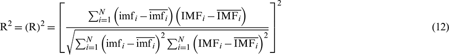
where  is the number of data,
  is the decomposition result of either the original or extension sequence, and
  is the decomposition result of the standard sequence.
RMSE, MAE, and MAPE measure the performance of models based on the difference between two variables–-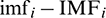 , and they pay attention to the deviation of data points from the standard. R and R-squared can show the degree of correlation between two sequences. This paper evaluates the performance of the CEEMDAN method for runoff sequences decomposition in each component. We not only concern the deviation of each data point from the standard, but also pay more attention to the correlation degree between the decomposition result and the standard sequence, that is, whether the decomposition results can accurately reflect the fluctuation trend and law contained in the standard sequence. In addition, there will be some data close to zero in the decomposition result and these data as the denominator will cause the evaluation result too large. R is appropriate for linear sequences, and R-squared is more broadly applicable. Therefore, we chose RMSE, MAE, and R-squared as indicators of performance evaluation.
3 Materials and Data Processing
In this study, we obtained the annual runoff series for Tangnaihai station from 1956 to 2013 and annual precipitation series for Dari station from 1956 to 2015, which are located in the source region of the Yellow River. The source region of the Yellow River is the most important area of runoff generation in the Yellow River basin. The evolution of hydrological elements in this region has a crucial influence on the change of water resources in the whole Yellow River basin. In addition, this area is less affected by human activities and the measured data of Tangnaihai station can reflect the runoff process under natural conditions. Therefore, the runoff characteristics here have unique and important research value. We use runoff data for our experiment and use rainfall data to verify the reliability of the method.
According to the characteristics of the original data, as well as for the convenience of the study, the measured runoff data were taken as the standard sequence, and the intercept data from 1962 to 2007 was taken as the original sequence. Then, the RBFNN extension method was applied to the original sequence to obtain the extension sequence. According to the interval in which the extreme point in the original sequence occurred, a period of seven years was chosen as the RBFNN prediction length at both ends to ensure that the prolongation contained a pair of extreme points and a certain precision was maintained. In the standard sequence, the portions of data from 1956 to 1962 and 2007 to 2013 were based on measured values which were regarded as the optimal continuation of the original sequence.
The extension of the original sequence of annual runoff as determined by RBFNN is shown in Fig. 1. The error of the RBFNN extension relative to the optimal extension is shown in Tab. 1.
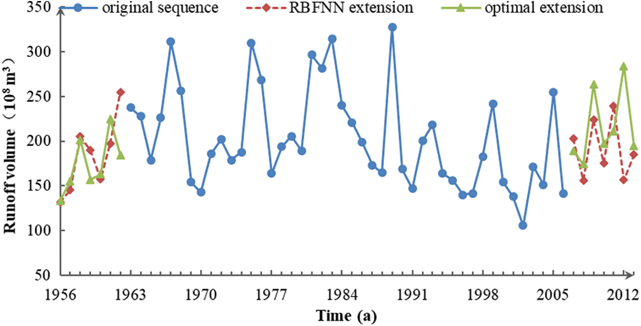
Figure 1: Three sets of runoff data. The measured data from 1962 to 2006 comprises the original sequence. The RBFNN extension is the continuation result of the original sequence and combines them to create the extension sequence. The points of optimal extension use the measured data from 1956 to 1962 and 2007 to 2013 in combination with the original sequence to get the standard sequence
Table 1: The effect of the extension compared with the optimal value on both sides

According to Fig. 1 and Tab. 1, of the six extreme points obtained from the right-side extension, only the sixth point was inconsistent with the real sequence, and the relative error reached 36.59%. This occurred because the maximum point and minimum point appeared alternately at the right end of the original sequence, and the RBFNN forecasting approach lengthens data with this rule. The 2012 data was contrary to the actual situation and resulted in errors. At the left end of the extension, there were three extreme points. The first point was discordant with the trend of the real series, and had a deviation of 37.96%. The RBFNN extension misjudged the occurrence of the first maximum. Beyond that, the other extreme points conformed to the change law of the actual sequence.
Endpoint extension is only an auxiliary tool and unnecessary to take a lot of time to pursue the prediction accuracy deliberately like specialized prediction research, so certain errors are acceptable. On the whole, the RBFNN extension series was close to the standard sequence, which approximately reflected the basic trend of the runoff series at the endpoint, with the exception of a few individual points.
4.1 Series Decomposition and Graphical Analysis
The annual runoff data from the original sequence, extension sequence, and standard sequence was individually decomposed using CEEMDAN. Figs. 2–6 show the decomposition results, where it can be seen that each sequence had four IMF components and one Res. Components of the extension sequence and standard sequence only retained the data from 1963 to 2006, and the data crippled by the endpoint effect at both ends was discarded. Moreover, the decomposition results of standard sequences can serve as criteria for comparison without the extension error.
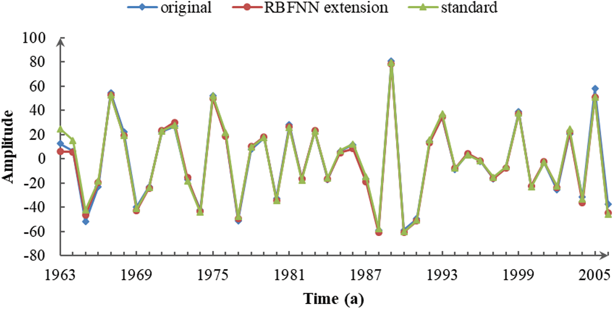
Figure 2: IMF1 of the three sequences decomposed by CEEMDAN
Figure 3: IMF2 of the three sequences decomposed by CEEMDAN
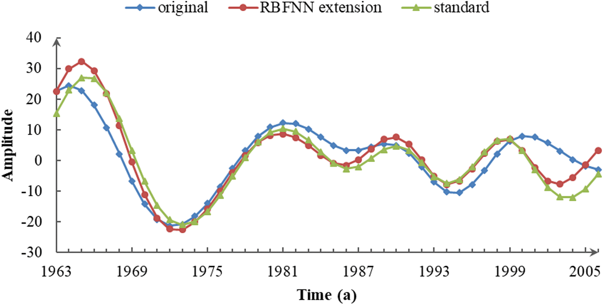
Figure 4: IMF3 of the three sequences decomposed by CEEMDAN

Figure 5: IMF4 of the three sequences decomposed by CEEMDAN

Figure 6: Res of the three sequences decomposed by CEEMDAN
Fig. 2 shows that each runoff series had a similar IMF1 component with high-frequency components that fluctuated over a quasi-periodicity of 2–5 years. The IMF1 component of the unprocessed original sequence slightly diverged from the standard sequence at both ends. By comparison, there was a more obvious separation between the extension sequence and standard sequence on the left side, which reflected the effect of the extension error. The comparison showed that the influence of the endpoint effect and the data extension on the decomposition accuracy was not obvious for the IMF1 component.
In Fig. 3, the three sequences displayed a uniform quasi-periodicity of 4–8 years. The data in the middle portions coincided, but both ends displayed a visible separation between the original and standard sequences caused by boundary error. The IMF2 component of the extension series was more accurate because the endpoint effect and extension error reflected in the IMF1 component were suppressed. Accordingly, it was concluded that the RBFNN extension improved the precision of the IMF2 component at the ends.
As seen in Fig. 4, the endpoint effect significantly reduced the accuracy of the medium-frequency IMF3 component. The fluctuation embodied in the original series was out of sync with the standard sequence, especially at the right end, and the quasi-periodicity was obviously larger. The decomposition result of the extension sequence remained consistent with the standard variation tendency, and separated at the two ends with only a small deviation in amplitude. In the IMF3 component, extending the original data effectively suppressed the error, and guaranteed the veracity of the information in the component, such as the quasi-periodicity of 9–16 years and other volatility characteristics.
Fig. 5 illustrates how the end effect led to the distortion of the IMF4 component extracted from the original sequence by CEEMDAN. The original sequence displayed the smallest amplitude and largest period, while the variation trend and the period of the extended sequence was consistent with the standard sequence, although the oscillation amplitude attenuated slightly. Consequently, in regard to the low-frequency IMF4 component, the RBFNN extension was still able to suppress the boundary error, reliably retain the primary trend or period information, and effectively reflect the amplitude within a certain degree.
As shown in Fig. 6, the three groups of residue all reflected a declining trend over an extended time scale, with only differing rates and ranges of change. In the middle portion, the standard sequence was closer to the extended data, while it was closer to the non-extended data at the margin. The residue of the original sequence reflected periodic characteristics and suggested that it may have a smaller period than the other series on a longer time scale.
Based on the above comparison and analysis, it can be seen that the error caused by the endpoint effect in CEEMDAN gradually propagated inward from the two ends as the decomposition proceeded. This then affected the decomposition result of the entire runoff series. The data extension technology did not visibly enhance the accuracy of the IMF1 component and residue. However, for other low and medium frequency components, the RBFNN extension significantly weakened the interference of the endpoint effect, inhibited internal propagation of the boundary error, improved the decomposition precision, and more accurately reflected the fluctuation characteristics in each time scale. At the end point in particular, the RBFNN extension truly revealed the trend of the data and conveniently provided the runoff prediction.
As previously stated, the decomposition results of the standard sequence and extended sequence only retained data from the years contained in the original sequence, so that their lengths were consistent. The decomposition result of the standard sequence was taken as the approximate value, and R, MAE and R-squared were used to measure the errors of the other two series. Tab. 2 shows the decomposition results.
Table 2: The decomposition accuracy of the original runoff sequence and extended sequence for IMF components 1–4 and the Res as quantified by RMSE, MAE and R-squared

As shown in Tab. 2, the decomposition accuracy of the extension sequence significantly improved when the endpoint effect was inhibited. In the IMF1 component, both sequences had high precision and there was no obvious advantage compared to data extension. Beyond that point, Tab. 2 outlines some interesting discoveries. As the decomposition progressed, the RMSE and MAE of IMF components 1–4 increased rapidly in the original series, and the error about the low frequency component quickly became out of control compared to the standard sequence. This eventually led to serious distortion of the decomposition results. The RMSE and MAE of the extended sequence were relatively stable and maintained a low level. Thus, the error in the low frequency component was effectively restrained. Regarding the Res component, although the RMSE of the two sequences were both larger than most of the IMF components, the decomposition accuracy of the extended sequence was still better. Of all the components, the extension sequence displayed higher R-squared values, especially in components IMF3 and IMF4. This indicated that its decomposition results more precisely reflected the fluctuation characteristics of the runoff series on different time scales.
In order to verify the reliability of the above methods, we performed RBFNN extension and CEEMDAN decomposition on the annual precipitation series of Dari stations. The extension results are shown in Fig. 7 and Tab. 3, and the decomposition results are shown in Fig. 8 and Tab. 4.

Figure 7: Three sets of annual precipitation data. The measured data from 1962 to 2008 comprises the original sequence. The RBFNN extension is the extension result of the original sequence and combines them to create the extension sequence. The points of optimal extension use the measured data from 1956 to 1962 and 2009 to 2015 in combination with the original sequence to get the standard sequence
Table 3: The effect of the extension compared with the optimal value on both sides


Figure 8: Three sequences of precipitation data decomposed by CEEMDAN
Table 4: The decomposition accuracy of the original precipitation sequence and extended sequence for IMF components 1–4 and the Res as quantified by RMSE, MAE and R-squared

It can be seen from the above that, although several points in the RBFNN extension deviated from the optimal sequence, the effect of CEEMDAN decomposition is still significantly better than that of the original sequence. Especially in Res component, the decomposition result of the original sequence is obviously distorted and even negatively correlated with the standard sequence. The trend of the extension sequence is consistent with the standard sequence and the endpoint effect is effectively suppressed. In other components, the experimental results of rainfall data and runoff data are similar, which verifies the reliability of the extension-decomposition method.
According to the comparison and analysis above, the use of the RBFNN extension technique to process the original data resulted in obvious improvement of the decomposition outcome. This improvement was important to the enhancement of the reliability of the multi-time scale analysis and runoff prediction.
From the perspective of the multi-time scale analysis, the endpoint effect disturbed the middle to low frequency IMF components of the original annual runoff, and the undulation features deviated significantly from the actual situation, causing distortion of information such as the amplitude and quasi-periodicity. The RBFNN extension for the runoff series increased the decomposition precision of the middle to low frequency components and maintained more authentic evolution rules for runoff on medium to long time scales, and provided a reliable basis for cycle identification and multi-time scale analysis in hydrologic research.
With regard to hydrological forecasting, utilization of the “decomposition–prediction–reconstruction” principle for prediction was influenced by the variation tendency at the ends of each component that guided the future direction and determined its prediction result. As the decomposition of the original sequence proceeded, the error at the boundary in each component increased, and when coupled with the distortion of the fluctuation information, the prediction accuracy decreased accordingly. Reconstruction of the prediction results will likely result in error superposition, which makes it difficult to achieve the desired forecasting effect. Hence, the use of data extension technology to improve the decomposition accuracy at the endpoint of a sequence is of great significance to achieve more accurate predictions for the “decomposition–prediction–reconstruction” method.
For other long hydrological data sequences, such as those composed of monthly or daily runoff, discarding the data points at both ends can theoretically restrain the endpoint effect [28]. However, this method will lead to missing data at the endpoints that is important to hydrological multi-time scale analysis and runoff forecasting. Deficient data at the right end makes the sequence unable to express the fluctuation characteristics of recent stream flow, which makes it difficult to provide assistance and guidance for current water resource utilization activities. In addition, a lack of data at the endpoints makes the subsequent trend of the series difficult to judge, increases the length of the prediction period, and reduces the accuracy of prediction. Extension of the runoff data can not only reduce the impact of the end effect, but also retain the original information at the endpoint, which is an ideal scheme for the improvement of the decomposition accuracy of CEEMDAN.
In summary, when using the CEEMDAN method to decompose hydrologic time series, it is necessary to extend the original sequence to improve the decomposition accuracy and improve the results of the hydrological analysis and forecast.
When analyzing hydrological multi-time scale features or runoff predictions, direct use of the CEEMDAN method to process nonlinear and non-stationary runoff sequences ignores the influence of the endpoint effects on decomposition accuracy and reduces the reliability and precision of the research. In this study, we adopted the RBFNN extension method to suppress the endpoint effect. Through analysis of the decomposition results of annual runoff sequences and annual precipitation sequences, we drew the following conclusions:
1. In the CEEMDAN method, the endpoint effect caused decomposition errors. As the decomposition proceeded, the error gradually propagated inward, which had a significant impact on the accuracy of the middle and low frequency components, especially at the endpoint, and resulted in information distortion.
2. The RBFNN extension technique used on the original data improved the decomposition accuracy of the low and medium frequency components and resulted in values similar to the ideal results in terms of fluctuation period and amplitude. This indicated that the fluctuation characteristics were accurately maintained in each time scale and the hydrological multi-time scale analysis was more realistic.
3. The extension sequence truly reflected the changing trend at the end of the components, which effectively guided their future direction. The utilization of the “extension–decomposition–prediction–reconstruction” process assisted in the exact prediction of the hydrologic time series.
Theoretically, the application of the “extension–decomposition–prediction–reconstruction” process is to combine the advantages of the CEEMDAN method for processing nonlinear data with the mature stationary sequence prediction technique to enhance the precision of complex hydrologic series prediction. Next, we will select an appropriate data extension technology and component prediction method to establish a new stream prediction model in order to achieve a more accurate forecast.
Funding Statement:This research is supported by the National Key R&D Program of China (Grant No. 2018YFC0406501), Outstanding Young Talent Research Fund of Zhengzhou University (Grant No. 1521323002), Program for Innovative Talents (in Science and Technology) at University of Henan Province (Grant No. 18HASTIT014), State Key Laboratory of Hydraulic Engineering Simulation and Safety, Tianjin University (Grant No. HESS-1717) and Foundation for University Youth Key Teacher of Henan Province (Grant No. 2017GGJS006).
Conflicts of Interest: The authors declare that they have no conflicts of interest to report regarding the present study.
1. Christensen, N. S., Wood, A. W., Voisin, N., Lettenmaier, D. P., Palmer, R. N. (2004). The effects of climate change on the hydrology and water resources of the Colorado River basin. Climate Change, 62(1–3), 337–363. DOI 10.1023/B:CLIM.0000013684.13621.1f. [Google Scholar] [CrossRef]
2. Abdul Aziz, O. I., Burn, D. H. (2006). Trends and variability in the hydrological regime of the Mackenzie River Basin. Journal of Hydrology, 319(1–4), 282–294. DOI 10.1016/j.jhydrol.2005.06.039. [Google Scholar] [CrossRef]
3. Lima, C. H. R., Lall, U. (2010). Spatial scaling in a changing climate: A hierarchical Bayesian model for non-stationary multi-site annual maximum and monthly streamflow. Journal of Hydrology, 383(3), 307–318. DOI 10.1016/j.jhydrol.2009.12.045. [Google Scholar] [CrossRef]
4. Zhang, Q., Gu, X. H., Singh, V. P., Xiao, M. Z., Chen, X. H. (2015). Evaluation of flood frequency under non-stationarity resulting from climate indices and reservoir indices in the East River basin, China. Journal of Hydrology, 527, 565–575. DOI 10.1016/j.jhydrol.2015.05.029. [Google Scholar] [CrossRef]
5. Sang, Y. F., Wang, Z. G., Liu, C. M. (2012). Period identification in hydrologic time series using empirical mode decomposition and maximum entropy spectral analysis. Journal of Hydrology, 424, 154–164. DOI 10.1016/j.jhydrol.2011.12.044. [Google Scholar] [CrossRef]
6. Wen, X. H., Feng, Q., Deo, R. C., Wu, M., Yin, Z. L. (2019). et al. Two-phase extreme learning machines integrated with the complete ensemble empirical mode decomposition with adaptive noise algorithm for multi-scale runoff prediction problems. Journal of Hydrology, 570, 167–184. DOI 10.1016/j.jhydrol.2018.12.060. [Google Scholar] [CrossRef]
7. Maheswaran, R., Khosa, R. (2012). Wavelet–Volterra coupled model for monthly stream flow forecasting. Journal of Hydrology, 450, 320–335. DOI 10.1016/j.jhydrol.2012.04.017. [Google Scholar] [CrossRef]
8. Kim, T. W., Valdes, J. B. (2003). Nonlinear model for drought forecasting based on a conjunction of wavelet transforms and neural networks. Journal of Hydrologic Engineering, 8(6), 319–328. DOI 10.1061/(ASCE)1084-0699(2003)8:6(319). [Google Scholar] [CrossRef]
9. Pagano, T. C., Wood, A. W., Ramos, M. H., Cloke, H. L., Pappenberger, F. (2014). et al. Challenges of operational river forecasting. Journal of Hydrometeorology, 15(4), 1692–1707. DOI 10.1175/JHM-D-13-0188.1. [Google Scholar] [CrossRef]
10. Mallat, S. G. (1989). A theory for multiresolution signal decomposition: The wavelet representation. IEEE Transactions on Pattern Analysis and Machine Intelligence, 11(7), 674–693. DOI 10.1109/34.192463. [Google Scholar] [CrossRef]
11. Mallat, S. G. (1998). A wavelet tour of signal processing. New York: Academic. [Google Scholar]
12. Huang, N. E., Long, S. R., Wu, M. L. C., Shih, H. H., Zheng, Q. N. (1998). The empirical mode decomposition and the Hilbert spectrum for nonlinear and non-stationary time series analysis. Proceedings of the Royal Society of London A: Mathematical, Physical and Engineering Sciences: The Royal Society, vol. 454, pp. 903–995. [Google Scholar]
13. Huang, N. E., Shen, Z., Long, S. R. (1999). A new view of nonlinear water waves: The Hilbert spectrum. Annual Review of Fluid Mechanics, 31(1), 417–457. DOI 10.1146/annurev.fluid.31.1.417. [Google Scholar] [CrossRef]
14. Karthikeyan, L., Kumar, D. N. (2013). Predictability of nonstationary time series using wavelet and EMD based ARMA models. Journal of Hydrology, 502(2), 103–119. DOI 10.1016/j.jhydrol.2013.08.030. [Google Scholar] [CrossRef]
15. Huang, N. E., Wu, Z. (2008). A review on Hilbert-Huang transform: Method and its applications to geophysical studies. Reviews of Geophysics, 46(2), RG2006. DOI 10.1029/2007RG000228. [Google Scholar] [CrossRef]
16. Sang, Y. F., Wang, Z., Liu, C. (2014). Comparison of the MK test and EMD method for trend identification in hydrological time series. Journal of Hydrology, 510(3), 293–298. DOI 10.1016/j.jhydrol.2013.12.039. [Google Scholar] [CrossRef]
17. Torres, M. E., Colominas, M. A., Schlotthauer, G., Flandrin, P. (2011). A complete ensemble empirical mode decomposition with adaptive noise. 2011 IEEE International Conference on Acoustics, Speech and Signal Processing (ICASSP), Prague, Czech Republic, pp. 4144–4147. [Google Scholar]
18. Wu, Z., Huang, N. E. (2009). Ensemble empirical mode decomposition: A noise-assisted data analysis method. Advances in Adaptive Data Analysis, 1(01), 1–41. DOI 10.1142/S1793536909000047. [Google Scholar] [CrossRef]
19. Marusiak, O., Pekar, J. (2014). Analysis of multiannual fluctuations and long term trends of hydrological time series, Greece. Proceedings of Advances in Environmental Sciences, Development and Chemistry, 17–21 July, Greece, pp. 156–159. [Google Scholar]
20. Zhang, W. Y., Qu, Z. X., Zhang, K. Q., Mao, W. Q., Ma, Y. N. (2017). et al. A combined model based on CEEMDAN and modified flower pollination algorithm for wind speed forecasting. Energy Conversion and Management, 136, 439–451. DOI 10.1016/j.enconman.2017.01.022. [Google Scholar] [CrossRef]
21. Adarsh, S., Janga, M. (2015). Multiscale analysis of suspended sediment concentration data from natural channels using the Hilbert–Huang Transform. Geoderma, 4, 780–788. [Google Scholar]
22. Liu, D., Chen, C., Qiang, F., Liu, C. L., Mo, L. (2018). et al. Multifractal detrended fluctuation analysis of regional precipitation sequences based on the CEEMDAN-WPT. Pure & Applied Geophysics, 175(8), 3069–3084. DOI 10.1007/s00024-018-1820-2. [Google Scholar] [CrossRef]
23. Zhang, J. P., Xiao, H. L., Zhang, X., Li, F. W. (2019). Impact of reservoir operation on runoff and sediment load at multi-time scales based on entropy theory. Journal of Hydrology, 569, 809–815. DOI 10.1016/j.jhydrol.2019.01.005. [Google Scholar] [CrossRef]
24. Norani, V., Baghanam, A. H., Adamowski, J., Kisi, O. (2014). Applications of hybrid wavelet-artificial intelligence models in hydrology: A review. Journal of Hydrology, 514, 358–377. DOI 10.1016/j.jhydrol.2014.03.057. [Google Scholar] [CrossRef]
25. Di, C., Yang, X., Wang, X. (2014). A four-stage hybrid model for hydrological time series forecasting. PLoS One, 9(8), e104663. DOI 10.1371/journal.pone.0104663. [Google Scholar] [CrossRef]
26. Zhang, H., Singh, V. P., Wang, B., Yu, Y. (2016). CEREF: A hybrid data-driven model for forecasting annual streamflow from a socio-hydrological system. Journal of Hydrology, 540, 246–256. DOI 10.1016/j.jhydrol.2016.06.029. [Google Scholar] [CrossRef]
27. Prasad, R., Deo, R. C., Li, Y., Maraseni, T. (2018). Soil moisture forecasting by a hybrid machine learning technique: ELM integrated with ensemble empirical mode decomposition. Geoderma, 330, 136–161. DOI 10.1016/j.geoderma.2018.05.035. [Google Scholar] [CrossRef]
28. Deng, Y. J., Wang, W., Qian, C. C., Wang, Z. Dai, J. D. (2001). et al. Boundary processing technique in EMD method and Hilbert transform. Chinese Science Bulletin, 46(1), l–8. [Google Scholar]
29. Zhao, J. P., Huang, D. J. (2001). Mirror extending and circular spline function for empirical mode decomposition method. Journal of Zhejiang University: Science A, 2(3), 247–252. DOI 10.1631/jzus.2001.0247. [Google Scholar] [CrossRef]
30. Shu, Z. H. P., Yang, Z. H. C. H. (2006). A better method for effectively suppressing end effect of empirical mode decomposition. Journal of Northwestern Polytechnical University, 24(5), 639–643. [Google Scholar]
31. Zhang, Y. S., Liang, J. W. (2003). Suppression of the end effect of empirical mode decomposition by using auto-regressive model. Science Development, 13(10), 1054–1059. [Google Scholar]
32. Hu, J. S., Yang, S. X. (2007). Application of EMD method with data extension technique based on RBF neural network to time-frequency analysis. Journal of Mechanical Strength, 29(6), 894–899. [Google Scholar]
33. Alizadeh, M. J., Kavianpour, M. R., Kisi, O., Nourani, V. (2017). A new approach for simulating and forecasting the rainfall-runoff process within the next two months. Journal of Hydrology, 548, 588–597. DOI 10.1016/j.jhydrol.2017.03.032. [Google Scholar] [CrossRef]
34. Elanayar, V. T., Shin, Y. C. (1994). Radial basis function neural network for approximation and estimation of nonlinear stochastic dynamic systems. IEEE Transactions on Neural Networks, 5(4), 594–603. DOI 10.1109/72.298229. [Google Scholar] [CrossRef]
35. Taormina, R., Galelli, S., Karakaya, G., Ahipasaoglu, S. D. (2016). An information theoretic approach to select alternate subsets of predictors for data-driven hydrological models. Journal of Hydrology, 542, 18–34. DOI 10.1016/j.jhydrol.2016.07.045. [Google Scholar] [CrossRef]
36. Colominas, M. A., Schlotthauer, G., Torres, M. E. (2014). Improved complete ensemble EMD: A suitable tool for biomedical signal processing. Biomedical Signal Processing and Control, 14, 19–29. DOI 10.1016/j.bspc.2014.06.009. [Google Scholar] [CrossRef]
37. Ren, Y., Suganthan, P. N., Srikanth, N. (2015). A comparative study of empirical mode decomposition-based short-term wind speed forecasting methods. IEEE Transactions on Sustainable Energy, 6(1), 236–244. DOI 10.1109/TSTE.2014.2365580. [Google Scholar] [CrossRef]
38. El-Shafie, A., Abdin, A. E., Noureldin, A., Taha, M. R. (2009). Enhancing inflow forecasting model at Aswan high dam utilizing radial basis neural network and upstream monitoring stations measurements. Water Resources Management, 23(11), 2289–2315. DOI 10.1007/s11269-008-9382-1. [Google Scholar] [CrossRef]
39. Parasuraman, K., Elshorbagy, A. (2007). Cluster-based hydrologic prediction using genetic algorithm-trained neural networks. Journal of Hydrologic Engineering, 12(1), 52–62. DOI 10.1061/(ASCE)1084-0699(2007)12:1(52). [Google Scholar] [CrossRef]
40. Hamdia, K. M., Ghasemi, H., Zhuang, X., Alajlan, N., Rabczuk, T. (2019). Computational machine learning representation for the flex electricity effect in truncated pyramid structures. Computers, Materials & Continua, 59(1), 79–87. DOI 10.32604/cmc.2019.05882. [Google Scholar] [CrossRef]
41. Hamdia, K. M., Ghasemi, H., Bazi, Y., AlHichri, H. Alajlan, N. (2019). et al. A novel deep learning based method for the computational material design of flexoelectric nanostructures with topology optimization. Finite Elements in Analysis and Design, 165, 21–30. DOI 10.1016/j.finel.2019.07.001. [Google Scholar] [CrossRef]
42. Guo, H. W., Zhuang, X. Y., Timon, R. (2019). A deep collocation method for the bending analysis of Kirchhoff plate. Computers, Materials & Continua, 59(2), 433–456. DOI 10.32604/cmc.2019.06660. [Google Scholar] [CrossRef]
43. Anitescu C., Atroshchenko E., Alajlan N., Rabczuk T. (2019). Artificial neural network methods for the solution of second ordeor boundary value problems. Computers, Materials & Continua, 59(1), 345–359. DOI 10.32604/cmc.2019.06641. [Google Scholar] [CrossRef]
44. Chai, T., Draxler, R. R. (2014). Root mean square error (RMSE) or mean absolute error (MAE)?–-Arguments against avoiding RMSE in the literature. Geoscientific Model Development, 7(3), 1247–1250. DOI 10.5194/gmd-7-1247-2014. [Google Scholar] [CrossRef]
45. Krause, P., Boyle, D., Bäse, F. (2005). Comparison of different efficiency criteria for hydrological model assessment. Advances in Geosciences, 5(5), 89–97. DOI 10.5194/adgeo-5-89-2005. [Google Scholar] [CrossRef]
 | This work is licensed under a Creative Commons Attribution 4.0 International License, which permits unrestricted use, distribution, and reproduction in any medium, provided the original work is properly cited. |