Engineering & Sciences
| Computer Modeling in Engineering & Sciences |
DOI: 10.32604/cmes.2021.012702
ARTICLE
The Equal-Norm Multiple-Scale Trefftz Method for Solving the Nonlinear Sloshing Problem with Baffles
1Department of Marine Engineering, National Taiwan Ocean University, Keelung, 202-24, Taiwan
2Department of Systems Engineering and Naval Architecture, National Taiwan Ocean University, Keelung, 202-24, Taiwan
3Center of Excellence for Ocean Engineering, National Taiwan Ocean University, Keelung, 202-24, Taiwan
*Corresponding Author: Yung-Wei Chen. Email: cyw0710@ntou.edu.tw
Received: 10 July 2020; Accepted: 09 February 2021
Abstract: In this paper, the equal-norm multiple-scale Trefftz method combined with the implicit Lie-group scheme is applied to solve the two-dimensional nonlinear sloshing problem with baffles. When considering solving sloshing problems with baffles by using boundary integral methods, degenerate geometry and problems of numerical instability are inevitable. To avoid numerical instability, the multiple-scale characteristic lengths are introduced into T-complete basis functions to efficiently govern the high-order oscillation disturbance. Again, the numerical noise propagation at each time step is eliminated by the vector regularization method and the group-preserving scheme. A weighting factor of the group-preserving scheme is introduced into a linear system and then used in the initial and boundary value problems (IBVPs) at each time step. More importantly, the parameters of the algorithm, namely, the T-complete function, dissipation factor, and time step, can obtain a linear relationship. The boundary noise interference and energy conservation are successfully overcome, and the accuracy of the boundary value problem is also improved. Finally, benchmark cases are used to verify the correctness of the numerical algorithm. The numerical results show that this algorithm is efficient and stable for nonlinear two-dimensional sloshing problems with baffles.
Keywords: Generalized lie-group method; multiple-scale Trefftz method; Laplace equation; baffled sloshing tank
With the continuous increase in global energy demand, the loading capacity of super-large oil tankers and floating production storage tanks are increasing. At the same time, the demand for liquefied petroleum gas carriers and liquefied natural gas carriers have increased, and the safety of the maritime navigation of liquid cargo ships has become a focus of interest. Early sloshing research mainly used experimental methods [1], but the corresponding disadvantages of high cost, long cycle, and complicated operation were greatly limited. In recent years, several methods for studying liquid sloshing have been proposed, by researchers such as Celebi et al. [2] and Frandsen [3], who used the finite difference method to simulate nonlinear sloshing problems in rectangular tanks. Wang et al. [4] used the finite element method (FEM) to address two-dimensional nonlinear sloshing problems with random excitations. Akyildiz et al. [5] used volumetric fluids to simulate the sloshing motion of a baffled tank and compared the results to those of experimental cases to analyse pressure changes on the wall of the tank. Biswal et al. [6] used the FEM to calculate the nonlinear sloshing response of a liquid in a two-dimensional rectangular tank with a rigid baffle. Younes et al. [7] used vertical baffled and holes in rectangular tanks for experimental studies. Maleki et al. [8] studied the effects of horizontal and vertical baffled on sloshing motion. However, there were some problems with these methods that need to be solved. For example, in the simulated fluid mechanics process, there are some complex problems, such as extreme deformation and free liquid surface, and motion interface. When meshing is applied for numerical simulation, element distortion will occur, and the calculation will not easily converge or will produce a considerable calculation error. Hence, some numerical methods have been proposed to construct approximate solutions without encountering these defects, such as the boundary element method [9], the Trefftz method [10], the modified Trefftz method [11], the radial basis function collocation method [12], the meshless method [13], and smooth particle hydrodynamics [14].
Recently, with the rapid development of computing technology, Sajedeh et al. [15] solved the nonlinear sloshing behaviour of a liquid in a partially filled tank which was studied using the FEM based on new spherical Hankel shape functions. Wang et al. [16] studied the nonlinear sloshing characteristics of the liquid contained in a tank with a vertical baffle mounted at the bottom of the tank. Han et al. [17] concerned with nonlinear sloshing in a partially filled container due to the three-dimensional vehicle motion. The liquid sloshing is described by a set of linear modal equations derived from the potential flow theory, which can be applied to liquid sloshing induced by an arbitrary combination of lateral, longitudinal, and rotational excitations. Guan et al. [18] simulated nonlinear sloshing in the three-dimensional tanks under horizontal excitation and roll excitation, and the inhibition effect of different baffles on the sloshing phenomenon was investigated. Jiang et al. [19] investigated the coupling effects of internal sloshing flow on the sway motion response of rectangular box sections. Three-dimensional sloshing simulation [20] was realized. The numerical accuracy was also improved, and the result was more reliable, but the main concern was the small-amplitude sloshing problem [21].
Some scholars began to explore the sloshing problem in other ways. Liu [22] proposed the modified Trefftz method to introduce a characteristic length in the T-complete basis function to improve numerical stability. Chen et al. [23] used the geometric multi-scale Trefftz method to solve the large-amplitude sloshing problem. Here, the concepts of the dissipation factor and control volume were first proposed to improve the accuracy of the solution. However, it is very expensive to obtain the dissipation factor and correction control volume. Chen [24] used the equal-norm multiple-scale Trefftz method (MSTM) in combination with the vector regularization method (VRM) to overcome boundary interference problems. With the development of group theory [25], many physical problems can be solved, such as coupling problems, boundary value problems, and ordinary differential equations. A group-preserving scheme (GPS) was one of the group theories, and Liu et al. [26] first derived the GPS based on the Lorentz group in the Minkowski space. However, the weighting factor of the GPS does not have linear properties; Liu [27] proved that the Lie-group scheme based on the general linear group in the Euclidean space was equivalent to the GPS in the Minkowski space. Hence, Chen et al. [28] proposed the MSTM combined with an explicit/implicit Lie-group scheme to overcome nonlinear sloshing behavior as well as to avoid the iterative correction of the controlled volume at each time step. Shih et al. [29] further extended the work [28] to verify nonlinear sloshing problems in two-dimensional rectangular and trapezoidaltanks.
Because degenerate geometry, energy conservation, and numerical instability problems exist in the nonlinear sloshing problems with baffles, a completely numerical procedure is constructed to address the initial and boundary value problems (IBVPs), respectively. First, when degenerate geometry and numerical instability problems occur in the boundary value problem (BVP), the T-complete basis function with different characteristic lengths and the VRM is applied to overcome boundary noise and high order numerical oscillations. Then, the explicit and implicit Lie group method in Euclidean space combined to perform time integration in the initial value problem (IVP) can avoid numerical iterative number, and the numerical solution of different time step by using the hybrid Lie group method has a linear relationship. Finally, for boundary noise disturbance and energy conservation at each time step, this paper introduces the weight factor of the IVP calculated by the GPS into the BVP to correct the dissipative factor. The new algorithm proposed in this paper will simultaneously overcome the above shortcomings.
2 A Trefftz Method for the Sloshing Problem
Assuming that the fluid is incompressible, nonrotating, and nonviscous, the potential flow theory can be used to describe sloshing in a tank, but the surface tension can be ignored. The sloshing problem assumes that the fluid in the tank is an ideal fluid, which satisfies the basic conditions of the potential flow theory, that is, the fluid in the tank is inviscid and non-rotational (irrotational) and incompressible properties and the fluid has continuity, therefore, it can be approximated by Laplace equation.
It is assumed that the free surface does not overturn or rupture during sloshing. W is the width of the rectangular tank, and D is the depth of the water, as shown in Fig. 1. The two coordinate systems are shown in Fig. 1. One coordinate system is an inertial Cartesian coordinate system (X, Z) fixed in space: the X-axis is horizontal, and the Z-axis is vertical. The other coordinate system is the moving coordinate system (x1, z1) connected to the tank; the observation point is at the intersection of the undisturbed free surface and the left wall of the tank. The tank is expected to have a translational oscillation along the X-axis, so the width of the flow is independent of the tank, which means that the sloshing of the liquid is only a two-dimensional nonlinear motion in the coordinate system. Considering the moving coordinate system fixed on the tank, the sloshing equation can be obtained as follows:
To describe the change in the free surface over time, where g is the gravitational acceleration and D is the vertical height difference between the liquid surface and the original liquid surface in the tank, A(t) is the external force term, and the swinging force of only the x1 component has a great influence on the dynamics of the tank due to the sloshing model of the tank moving along the x1-axis. In this paper, the rocking forces acting on the left and right walls are considered. Assuming that the normal velocity at the bottom of the tank and the boundary velocity between the two side walls are zero, the boundary conditions of the tank wall are as follows:
where

Figure 1: The rectangular tank (a) sketch and (b) characteristic lengths
For the convenience of description, polar coordinates are used here. The governing equations and boundary conditions are expressed as follows:
Since the governing equation for the sloshing problem is a two-dimensional Laplace equation, we can use the linear combination of T-complete functions to express the numerical solution. The T-complete functions of the two-dimensional Laplace equation can be shown as:
where
where
where
In this paper, we introduce the collocation method. Eqs. (7) and (8) are imposed at different collocation points on two different boundaries with [r(θ), θ] ∈ ΓF and [r(
where
where for simple description
where
where
where
Combining Eq. (10) into the linear system with n = 2m + 1 dimensions, where m is a positive integer that can be selected according to the problem, the linear system in Eq. (11) can be written as follows:
where B is the coefficient matrix of the linear system,
3 A Vector Regularization Method (VRM)
When a matrix is ill-posed and the measured data contain noisy disturbances, it is difficult to determine the stability of the system using conventional regularization techniques. Therefore, Liu et al. [31] proposed VRM, which proves that a solution exists when we have an ill-posed matrix and noisy disturbances occur. Considering that a given matrix B or V is an inversion of B and that
where
When the regularization parameter is
When combining Eqs. (14) and (16), the over-determined system can be written as
where
Multiplying Eq. (16) by
According to the matrix operators in Eq. (18) applied to
Changing B of the above formula to BT, a linear equation equivalent to Eq. (13) can be obtained as follows:
For the convenience of calculation, Eq. (20) is expressed as
where
To maintain energy conservation and no volume correction, a weighting factor in the group preservation algorithm can be obtained:
where
where
Finally, the conjugate gradient method (CGM) is used to solve for q in Eq. (23).
4 An Explicit/Implicit Lie-Group Scheme
Eqs. (2)–(4) in vector form are as follows:
where u and v are as follows:
According to the formulas by Liu [27], an explicit scheme based on the Lie-group (ESGL) is used for the integration of the nonlinear dynamical system in Eq. (24), which can be used to derive the following scheme:
where
On the other hand, we applied an implicit scheme based on the Lie-group (ISGL) for the integration of the nonlinear dynamical system in Eq. (24); the simplest one considers
where
With
If
Then, for
In this section, three benchmark numerical examples are examined to verify the numerical algorithm.
All numerical experiments are tested on Intel (R) Xeon(R) E31230 CPU clocked at 3.2GHz with 32 GB of RAM. The external excitation is a horizontal displacement given by
Thus, the first natural frequency of this tank is
Before testing the effects of baffles and screens on sloshing damping, we consider two-dimensional rectangular tank sloshing without any obstacles. The length of the 2-D rectangular tank in the X direction is W = 0.9 m. Initially, the static water in the tank has a depth of D = 0.6 m. To verify the accuracy, we compare with the results of the literature [32,33]. The depth of the water in the literature of the sloshing amplitude was 0.6. For ease of comparison in this paper, unified the water surface height as 0 at the static water, and the difference between the two water levels is shown in Fig. 2, which presents the vertical displacement of the free-surface point in contact with the left wall for two different excitation frequencies. The analytical solution proposed by Chen et al. [32] is also represented in the same figures. The agreement between the numerical and the analytical results is satisfactory. When the excitation frequency is close to the resonance frequency, a beating phenomenon appears. The frequency of the beating of the amplitude-modulated wave is

Figure 2: Comparison of two numerical simulations and the analytical solution of the free surface elevation at the left wall: (a)
The traditional Trefftz method usually increases the dissipation factor to improve instability by adding a smoothing term or a dissipation term, but the dissipation coefficient should not be too large, otherwise numerical instability will occur. In the simulation of large-amplitude sloshing problems, the instability can be overcome by reducing the time step and simultaneously reducing the dissipation factor. In most of the numerical models used in the past, the selection of the dissipation factor and the time step often need to be conservative to avoid calculation instability.
In the long-term simulation of the nonlinear sloshing problem, the traditional method is time-consuming. The proposed method can adjust the parameters and save computation time, and the result is stable under long-term calculation. This model simulates the sloshing problem under different conditions by changing the time step and the dissipation factor. Here, we consider the time steps of 5 series to be 1.0e−2, 1.0e−3, 5.0e−4, 1.0e−4, and 1.0e−5, respectively, as shown in Fig. 5. The dissipative factor of the method has a linear relationship with the time step, and the method is verified to have a relational expression of

Figure 3: When

Figure 4: The wave history on the tank’s walls under forced vibration; the period of the beating is 101.2 s
When approaching the resonant frequency, in Fig. 7a and the parameters are as follows: tank width W = 1.0 (m), static water depth D = 0.5 (m), dissipation factor
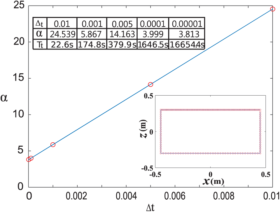
Figure 5: A linear relationship between the dissipation factor and the time step under
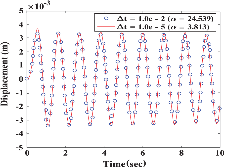
Figure 6: Comparison considering different dissipation factors and time steps under
Because the free surface is not easily disturbed by the transient external force, we consider the harmonic force and transient force simultaneously. Fig. 8 was shown the 3 transient pulse waves (at 2.5, 5, and 7.5 s) with the sloshing simulation in 10 s. In this case the large harmonic excitation amplitude d = 0.01 m, and the transient pulse wave amplitude d = 0.1 m. Comparison with transient wave excitation and without transient wave excitation, the simulation results are shown in Figs. 9a and 9b. The result proves that this method is not affected by the external transient wave excitation and still maintains stability. It can be seen from Figs. 7–9 that the method can obtain stable and correct solutions regardless of the simulation results of large amplitude, small amplitude, or burst waves, which proves that the method is indeed effective in a variety of external force excitation modes.
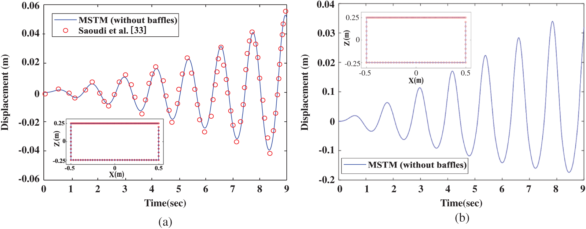
Figure 7: (a) Comparison of the free surface elevation at the left wall determined by the present numerical solution and the work of Saoudi et al. [33]. (b) Large amplitudes of the free surface elevation at the left wall
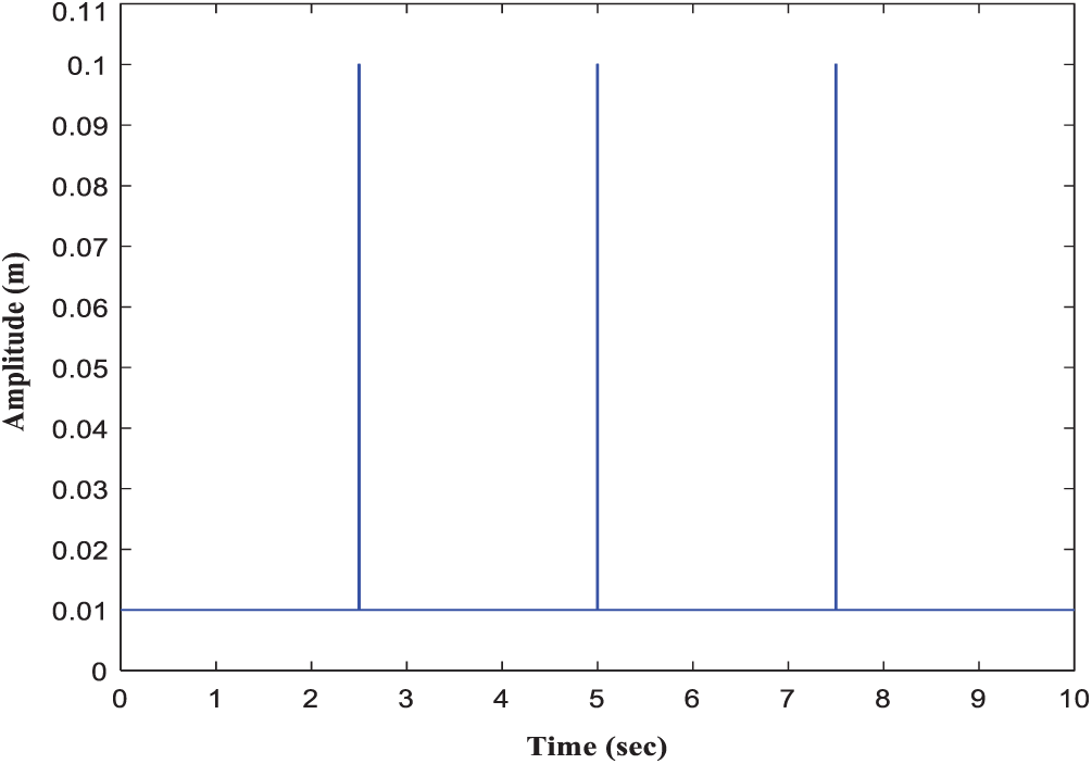
Figure 8: Input 3 large amplitude transient pulse waves within 10 seconds (at 2.5, 5 and 7.5 s)
5.1 Simulation of Rectangular Tanks with a Baffle
For simulating the sloshing problem under an external force, the tank model was shown in Fig. 1a sketch of the baffled tanks was shown in Fig. 10. The parameters were shown as follows: D = 0.5 m, W = 1.0 m, T = 0.01 m, d = 0.002 m and
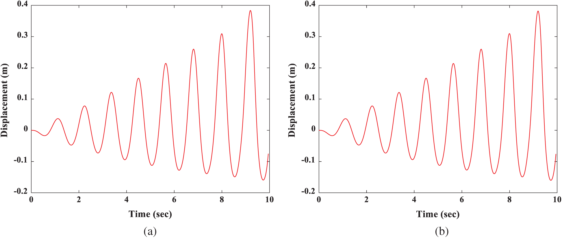
Figure 9: Comparison with large amplitude of (a) with 3 transient pulse wave (at 2.5, 5 and 7.5s) (b) without transient pulse wave in 10 s at the right wall
The numerical results of the free surface displacement on the right end of the tank are compared with the numerical results described by Liu et al. [34]. The results are shown to be in good agreement. To test the accuracy and stability of the algorithm, it was found that the results analysed by this algorithm, as shown in Fig. 13a, are very consistent with the results of other methods before
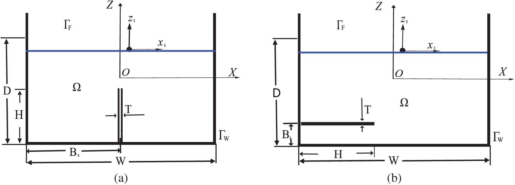
Figure 10: Sketch of baffled tanks: (a) vertical and (b) horizontal
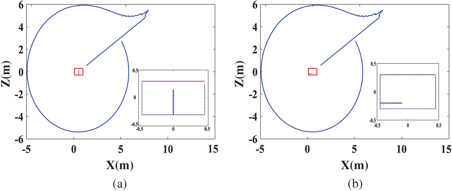
Figure 11: The initial contours of the characteristic lengths and collocation points in rectangular baffled tanks: (a) vertical and (b) horizontal

Figure 12: Comparison of the calculation results of a single vertical baffled tank from the proposed method and the literature (a) middle location (b) left location
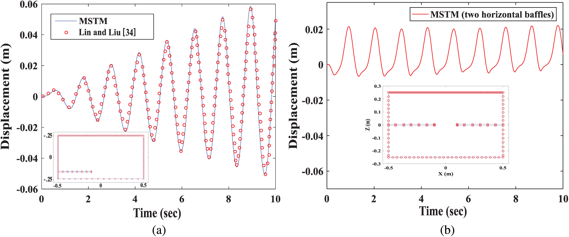
Figure 13: The numerical results of a rectangular tank with horizontal baffles: (a) one and (b) two
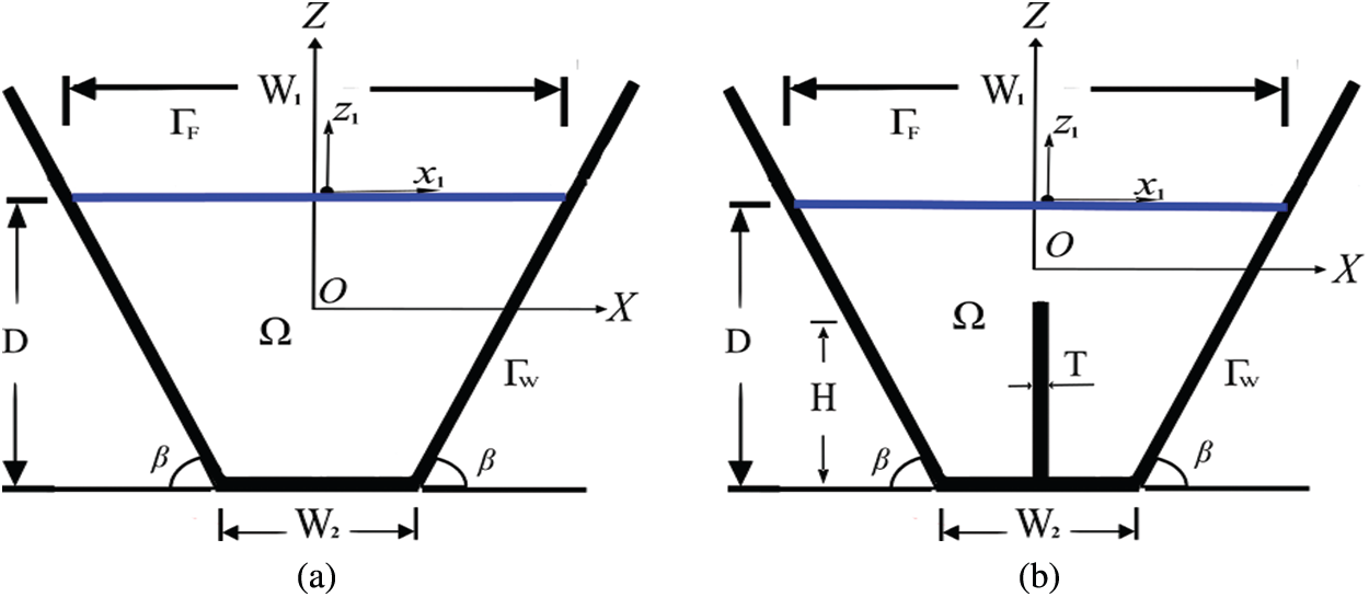
Figure 14: Sketch of baffled tanks: (a) empty (b) vertical baffle
5.2 Simulation of a Trapezoidal Tank
According to the results described by Mitra et al. [35], the basic sloshing frequency is calculated to be 2.39 rad/s when the static water depth in the trapezoidal tank is H = 4 m. To show that the method has high precision and stability under large-amplitude sloshing, the trapezoidal tanks considered here are shown in Fig. 14: the static water depth is D = 4 m, and the tank surface width is W1 = 6.0 m. The vertical baffle with a thickness of T = 0.01 m is located in the middle of the trapezoidal tank, the bottom width of the tank is W2 = 2.0 m, and
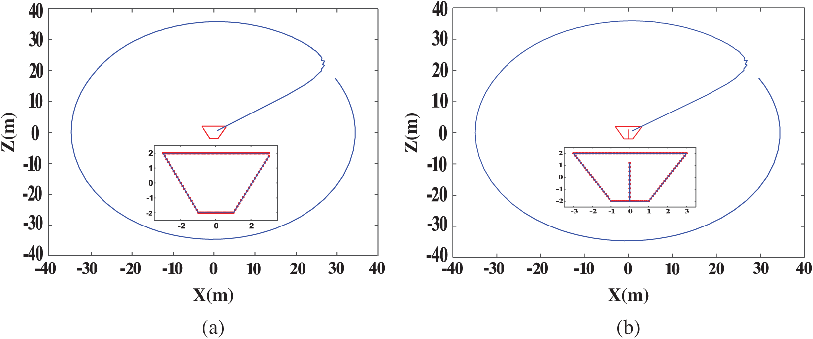
Figure 15: The initial contours of the characteristic lengths and collocation points in trapezoidal baffled tanks: (a) vertical and (b) horizontal
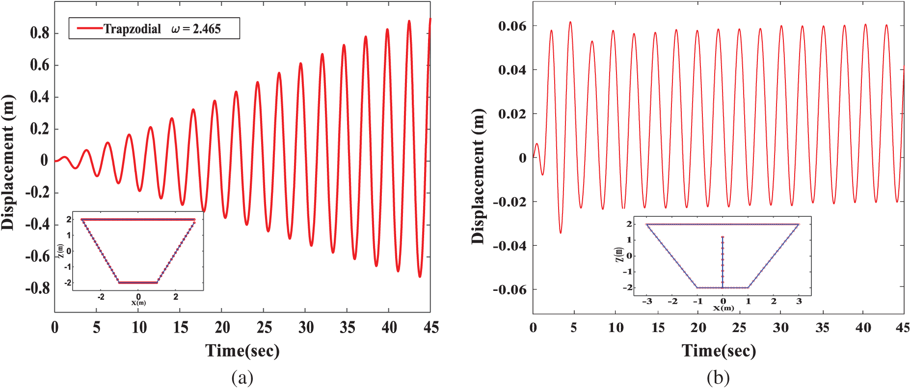
Figure 16: The elevation of the free surface of the trapezoidal tank with resonance frequency (a)without baffles (b) with a single vertical baffled
In this study, the MSTM is used to solve the nonlinear sloshing problem of the baffled tank and combines the explicit/implicit Lie-group scheme to integrate into the time domain to accurately perform the simulation analysis. When the time integration scheme based on the generalized linear group is used for time integration, the nonlinear term of the free surface boundary condition can be easily handled. This algorithm successfully improves the computational efficiency and stability of the solutions for the IVP and BVP when considering a baffle with a large aspect ratio. In this paper, five cases are used to verify the numerical stability of this simulation model, including two standard sloshing tests and three single-baffle sloshing tests. The numerical results are compared with the previous literature, and numerical results of different parameters are carried out in these cases. The numerical results show that overcoming the problem of small geometric scales and finding a linear relationship between the dissipation factor and the time step can make it easier for users to solve problems. Hence, the MSTM combined with the explicit/implicit Lie-group scheme not only easily and effectively solves this problem but also successfully simulates the nonlinear baffled tank sloshing problem under various conditions.
Funding Statement: The second author greatly appreciates the financial support provided by the Ministry of Science and Technology, Taiwan, ROC, under Contract No. MOST 108-2221-E-019-015.
Conflicts of Interest: The authors declare that they have no conflicts of interest to report regarding the present study.
1. Abramson, M. N., Chu, W. H., Kana, D. D. (1966). Some studies of nonlinear lateral sloshing in rigid containers. Journal of Applied Mechanics, 33(4), 777–784. DOI 10.1115/1.3625182. [Google Scholar] [CrossRef]
2. Celebi, M. S., Akyildiz, H. (2002). Nonlinear modelling of liquid sloshing in a moving rectangular tank. Ocean Engineering, 29(11), 1527–1553. DOI 10.1016/S0029-8018(01)00085-3. [Google Scholar] [CrossRef]
3. Frandsen, J. B. (2004). Sloshing motions in excited tanks. Journal of Computational Physics, 196(1), 53–87. DOI 10.1016/j.jcp.2003.10.031. [Google Scholar] [CrossRef]
4. Wang, C. Z., Khoo, B. C. (2005). Finite element analysis of two-dimensional nonlinear sloshing problems in random excitations. Ocean Engineering, 32(2), 107–133. DOI 10.1016/j.oceaneng.2004.08.001. [Google Scholar] [CrossRef]
5. Akyildiz, H., Unal, N. E. (2006). Sloshing in a three-dimensional rectangular tank. Numerical Simulation and Experimental Validation Ocean Engineering, 33(15), 2135–2149. DOI 10.1016/j.oceaneng.2005.11.001. [Google Scholar] [CrossRef]
6. Biswal, K. C., Bhattacharyya, S. K., Sinha, P. K. (2006). Nonlinear sloshing in partially liquid filled containers with baffled. International Journal for Numerical Methods in Engineering, 68(3), 317–337. DOI 10.1002/nme.1709. [Google Scholar] [CrossRef]
7. Younes, M. F., Younes, Y. K., Madah, M. E., Ibrahim, I. M., Dannanh, E. E. (2007). An experimental investigation of hydrodynamic damping due to vertical baffle arrangements in a rectangular tank. Proceedings of the Institution of Mechanical Engineers Part M: Journal of Engineering for the Maritime Environment, 221(3), 115–123. DOI 10.1243/14750902JEME59. [Google Scholar] [CrossRef]
8. Maleki, A., Ziyaeifar, M. (2008). Sloshing damping in cylindrical liquid storage tanks with baffles. Journal of Sound and Vibration, 311(1–2), 372–385. DOI 10.1016/j.jsv.2007.09.031. [Google Scholar] [CrossRef]
9. Gedikli, A., Ergüven, M. E. (2003). Evaluation of sloshing problem by variational boundary element method. Engineering Analysis with Boundary Elements, 27(9), 935–943. DOI 10.1016/S0955-7997(03)00046-8. [Google Scholar] [CrossRef]
10. Kita, E., Katsuragawa, J., Kamiya, N. (2004). Application of Trefftz-type boundary element method to simulation of two-dimensional sloshing phenomenon. Engineering Analysis with Boundary Elements, 28(6), 677–683. DOI 10.1016/j.enganabound.2003.07.003. [Google Scholar] [CrossRef]
11. Chen, Y. W., Liu, C. S., Chang, C. M., Chang, J. R. (2010). Application of the modified Trefftz method to the simulation of sloshing behaviors. Engineering Analysis with Boundary Elements, 34(6), 581–598. DOI 10.1016/j.enganabound.2010.01.003. [Google Scholar] [CrossRef]
12. Wu, N. J., Chang, K. A. (2011). Simulation of free-surface waves in liquid sloshing using a domain-type meshless method. International Journal for Numerical Methods in Fluids, 67(3), 269–288. DOI 10.1002/fld.2346. [Google Scholar] [CrossRef]
13. Pal, P. (2012). Slosh dynamics of liquid-filled rigid containers: Two-dimensional meshless local Petrov–Galerkin approach. ASCE Journal of Engineering Mechanics, 138(6), 567–581. DOI 10.1061/(ASCE)EM.1943-7889.0000367. [Google Scholar] [CrossRef]
14. Shao, J. R., Li, H. Q., Liu, G. R., Liu, M. B. (2012). An improved SPH method for modelling liquid sloshing dynamics. Computers and Structures, 100, 18–26. DOI 10.1016/j.compstruc.2012.02.005. [Google Scholar] [CrossRef]
15. Sajedeh, F., Mahnaz, G. H., Saleh, H. J. (2019). Developing new numerical modelling for sloshing behaviour in two-dimensional tanks based on nonlinear finite-element method. Journal of Engineering Mechanics, 145(12), 4019107. DOI 10.1061/ASCE(EM). 1943-7889.0001686. [Google Scholar] [CrossRef]
16. Wang, J. H., Sun, S. L. (2019). Study on liquid sloshing characteristics of a swaying rectangular tank with a rolling baffle. Journal of Engineering Mathematics, 119(1), 23–41. DOI 10.1007/s10665-019-10017-7. [Google Scholar] [CrossRef]
17. Han, M., Dai, J., Wang, C. M., Ang, K. K. (2019). Hydrodynamic analysis of partially filled liquid tanks subject to 3D vehicular manoeuvring. Shock and Vibration, 2019, 1–14. DOI 10.1155/2019/6943879. [Google Scholar] [CrossRef]
18. Guan, Y., Yang, C., Chen, P., Zhou, L. (2020). Numerical investigation on the effect of baffles on liquid sloshing in 3D rectangular tanks based on nonlinear boundary element method. International Journal of Naval Architecture and Ocean Engineering, 12, 399–413. DOI 10.1016/j.ijnaoe.2020.04.002. [Google Scholar] [CrossRef]
19. Jiang, S. C., Bai, W. (2020). Coupling analysis for sway motion box with internal liquid sloshing under wave actions. Physics of Fluids, 32(7), 72106. DOI 10.1063/5.0015058. [Google Scholar] [CrossRef]
20. Wu, G. X., Ma, Q. W., Taylor, R. E. (1998). Numerical simulation of sloshing waves in 3D tank based on a finite element method. Applied Ocean Research, 20(6), 337–355. DOI 10.1016/S0141-1187(98)00030-3. [Google Scholar] [CrossRef]
21. Miao, Y., Wang, S. (2014). Small amplitude liquid surface sloshing process detected by optical method. Optics Communications, 315(14), 91–96. DOI 10.1016/j.optcom.2013.10.079. [Google Scholar] [CrossRef]
22. Liu, C. S. (2007). A modified Trefftz method for two-dimensional Laplace equation considering the domain’s characteristic length. Computer Modelling in Engineering & Sciences, 21, 53–62. DOI 10.3970/cmes.2007.021.053. [Google Scholar] [CrossRef]
23. Chen, Y. W., Yeih, W. C., Liu, C. S., Chang, J. R. (2012). Numerical simulation of the two-dimensional sloshing problem using a multi-scaling Trefftz method. Engineering Analysis with Boundary Elements, 36(1), 9–29. DOI 10.1016/j.enganabound.2011.07.009. [Google Scholar] [CrossRef]
24. Chen, Y. W. (2016). A multiple scale Trefftz method for the Laplace equation subjected to large noisy boundary data. Engineering Analysis with Boundary Elements, 64(5), 196–204. DOI 10.1016/j.enganabound.2015.12.009. [Google Scholar] [CrossRef]
25. Hall, B. C. (2015). Lie groups, lie algebras, and representations: An element introduction. Graduate Texts in Mathematics, 222, 351. DOI 10.1007/ISBN978-3-319-13467-3. [Google Scholar] [CrossRef]
26. Liu, C. S. (2001). Cone of nonlinear dynamical system and group preserving schemes. International Journal of Nonlinear Mechanics, 36(7), 1047–1068. DOI 10.1016/S0020-7462(00)00069-X. [Google Scholar] [CrossRef]
27. Liu, C. S. (2013). A method of Lie-symmetry GL (n, R) for solving nonlinear dynamical systems. International Journal of Nonlinear Mechanics, 52, 85–95. DOI 10.1016/j.ijnonlinmec.2013.01.015. [Google Scholar] [CrossRef]
28. Chen, Y. W., Shih, C. F., Liu, Y. C., Soon, S. P. (2019). An explicit/implicit lie-group scheme for solving problems of nonlinear sloshing behaviours. International Journal of Offshore Polar Engineering, 29(1), 42–52. DOI 10.17736/ijope.2019.mk62. [Google Scholar] [CrossRef]
29. Shih, C. F., Chen, Y. W., Soon, S. P., Ho, S. Y. (2019). A numerical study of the effects of the baffles on liquid sloshing in two-dimensional tanks. Proceedings of the Twenty-Ninth International Ocean and Polar Engineering Conference, pp. 3386–3392. Honolulu, Hawaii, USA. [Google Scholar]
30. Liu, C. S. (2008). A highly accurate MCTM for inverse Cauchy problems of Laplace equation in arbitrary plane domains. Computer Modelling in Engineering & Sciences, 35(2), 91–111. DOI 10.17207/jstc.2008.11.18.91. [Google Scholar] [CrossRef]
31. Liu, C. S., Hong, H. K., Atluri, S. N. (2010). Novel algorithms based on the conjugate gradient method for inverting ill-conditioned matrices, and a new regularization method to solve ill-posed linear systems. Computer Modeling in Engineering & Sciences, 60(3), 279–308. DOI 10.3970/cmes.2010.060.279. [Google Scholar] [CrossRef]
32. Chen, B. F., Nokes, R. (2005). Time-independent finite difference analysis of fully nonlinear and viscous fluid sloshing in a rectangular tank. Journal of Computational Physics, 209(1), 47–81. DOI 10.1016/j.jcp.2005.03.006. [Google Scholar] [CrossRef]
33. Saoudi, M. Z., Hafsia, Z., Maalel, K. (2013). Dumping effects of submerged vertical baffles and slat screen on forced sloshing. Journal of Water Resource and Hydraulic Engineering, 2(2), 51–60. [Google Scholar]
34. Liu, D., Lin, P. (2009). Three-dimensional liquid sloshing in a tank with baffled. Ocean Engineering, 36(2), 202–212. DOI 10.1016/j.oceaneng.2008.10.004. [Google Scholar] [CrossRef]
35. Mitra, S., Upadhyay, P. P., Sinhamahapatra, K. P. (2008). Slosh dynamics of inviscid fluids in two-dimensional tanks of various geometry using finite element method. International Journal for Numerical Methods in Fluids, 56(9), 1625–1651. DOI 10.1002/fld.1561. [Google Scholar] [CrossRef]
 | This work is licensed under a Creative Commons Attribution 4.0 International License, which permits unrestricted use, distribution, and reproduction in any medium, provided the original work is properly cited. |