Engineering & Sciences
| Computer Modeling in Engineering & Sciences |
DOI: 10.32604/cmes.2021.015694
ARTICLE
Bilateral Filter for the Optimization of Composite Structures
1State Key Laboratory of Digital Manufacturing Equipment and Technology, Huazhong University of Science and Technology, Wuhan, China
2State Key Laboratory of Structural Analysis for Industrial Equipment, Dalian University of Technology, Dalian, China
*Corresponding Author: Qi Xia. Email: qxia@mail.hust.edu.cn
Received: 06 January 2021; Accepted: 08 March 2021
Abstract: In the present study, we propose to integrate the bilateral filter into the Shepard-interpolation-based method for the optimization of composite structures. The bilateral filter is used to avoid defects in the structure that may arise due to the gap/overlap of adjacent fiber tows or excessive curvature of fiber tows. According to the bilateral filter, sensitivities at design points in the filter area are smoothed by both domain filtering and range filtering. Then, the filtered sensitivities are used to update the design variables. Through several numerical examples, the effectiveness of the method was verified.
Keywords: Design optimization; composite structure; fiber angle optimization; bilateral filtering; Shepard interpolation; manufacturability constraints
Advanced manufacturing technologies of fiber-reinforced composite structures, for instance the automatic tape laying (ATL) and automatic fiber placement (AFP), allow composite structures to be manufactured with curvilinear fibers [1,2]. Therefore, stiffness can be different at different positions of the structure, and the freedom for improving the structural performance is larger than the constant stiffness composite structures [3–5]. However, the gap/overlap and excessive curvature of curvilinear fiber tows give rise to the appearance of manufacturing defects. The issue should be carefully dealt with at the design stage. When curvilinear fiber tows are not parallel [6–9], gaps and overlaps between adjacent fiber tows will appear. When the curvature of the fiber tow is too large, the tension and compression on the edges of the fiber tows will result in delamination and wrinkling [10,11].
How to avoid such defects has become an important topic in the design optimization of composite structures with curvilinear fibers, and many efforts have been made in recent years. Brampton et al. [8] employed the isolines of level set function to represent equally spaced fiber paths, hence preventing gaps/overlaps. Brooks et al. [11] treated fiber paths as the streamlines of a vector field, and gaps/overlaps and curvatures are respectively controlled by the constraints of the curl and divergence of this vector field. Hao et al. [12] proposed a multi-stage design strategy based on lamination parameters, in which the curvature and parallelism constraints were formulated as inequalities by using path functions. Hong et al. [13] developed an approach that controls the curvature of a fiber path through the gradient of lamination parameters. Tian et al. [14] proposed a parametric divergence-free vector field (pDVF) method for the optimization of fiber angle arrangement, and it ensures that fibers in one-ply do not cross each other.
In our previous study, within the Shepard-interpolation-based framework for design optimization, a gap/overlap constraint and a curvature constraint were proposed [15]. However, the two constraints should be defined at each design point, thus there are a large number of constraints, and the optimization is not efficient. In order to enhance the optimization efficiency, in [16] two filters were proposed to address the issue of gap/overlap and excessive curvature. At each design point, the sensitivity is first filtered in a rectangular region around the point, and by this means the fiber curvature is controlled. Then, in another rectangular region around the point, the filtered sensitivities are averaged to ensure fibers parallel to each other. Finally, the resulting sensitivity information is used to update the design variable.
In the present study, we propose to integrate the bilateral filter into the Shepard-interpolation-based fiber angle optimization (SFAO) [17,18]. According to the bilateral filter, a circular area is defined at each design point, and sensitivities at design points in the circular area are smoothed by both domain filtering and range filtering. The domain filtering is responsible for smoothing the magnitude of sensitivities, and the range filtering is responsible for adaptively adjusting the strength of smoothing according to the difference of fiber angles. The filtered sensitivities are used to update the design variables. As compared to the two-filter approach in our previous study [16], the bilateral filter approach is simpler and more convenient. In addition, the bilateral filter developed for image processing [19–21] has also been applied to the SIMP (Solid Isotropic Material with Penalization) [22,23] method for structural topology optimization, and it was proved to be effective to suppress the checkerboard pattern and simultaneously obtain a high-contrast black-white pattern of structure.
In this paper, the minimum compliance problem defined in Eq. (1) is considered
where
Inspired by Kang et al. [24,25], the Shepard interpolation was proposed in our previous study to describe the fiber angles in the design domain. The fiber angles at finite element centers are computed by using a continuous function. This function is constructed by the Shepard method that interpolates the fiber angles at scattered design points, and it is given by [18]
where
where
Another useful property of Shepard interpolation is expressed as
According to Eq. (4), when the fiber angle at any point in the design domain needs to be constrained as
The equilibrium equation
where
where
3 Sensitivity Analysis and Bilateral Filter
The sensitivity of the objective function with respect to design variables is given by [18]
The derivative of the fiber angle
where
After the sensitivity of each design variable
The bilateral filtering of sensitivities is written as
where Ni is the circular filtering area centered at the design point i;
where
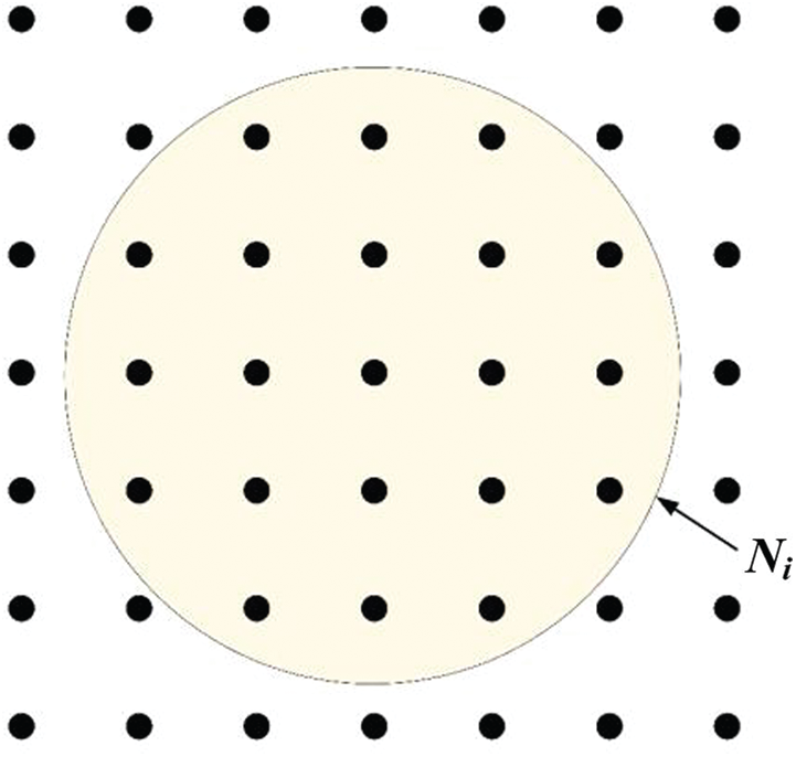
Figure 1: Schematic diagram of the sensitivity bilateral filtering area (the black dots represent the design points)
In this section, the proposed optimization method is applied to several 2D structures subjected to in-plane loads. In these examples, the mechanical properties of the composite material are assumed as Ex = 1, Ey = 0.05, Gxy = 0.03, vxy = 0.3, vxy = 0.015. Plane-stress quadrilateral elements are used for the finite element analysis, and self-weight of the structure is not considered. The criterion of convergence is that the number of iterations is no more than 50. According to our experience, 50 iterations are enough for convergence. When the initial value of the fiber angle is set as
The fiber angle distribution obtained by the optimization is post-processed by using the Tecplot software to generate fiber paths. In fluid dynamics, it is well known that the velocity of any point in a flow field is tangent to the streamline through the point. For the element e in the design domain, a vector at the element center is defined by
This vector is tangent to the fiber path through the element center. After importing the vector field constructed by Eq. (13), the Tecplot generates fiber paths.
The first design problem is shown in Fig. 2. The size of the design domain is
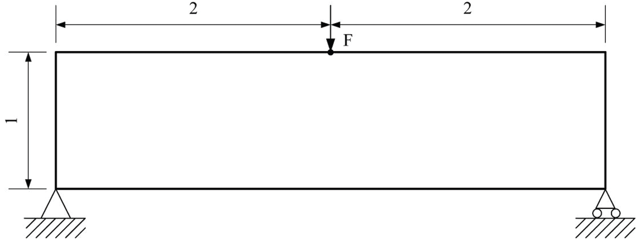
Figure 2: Design problem of the first example
Firstly,
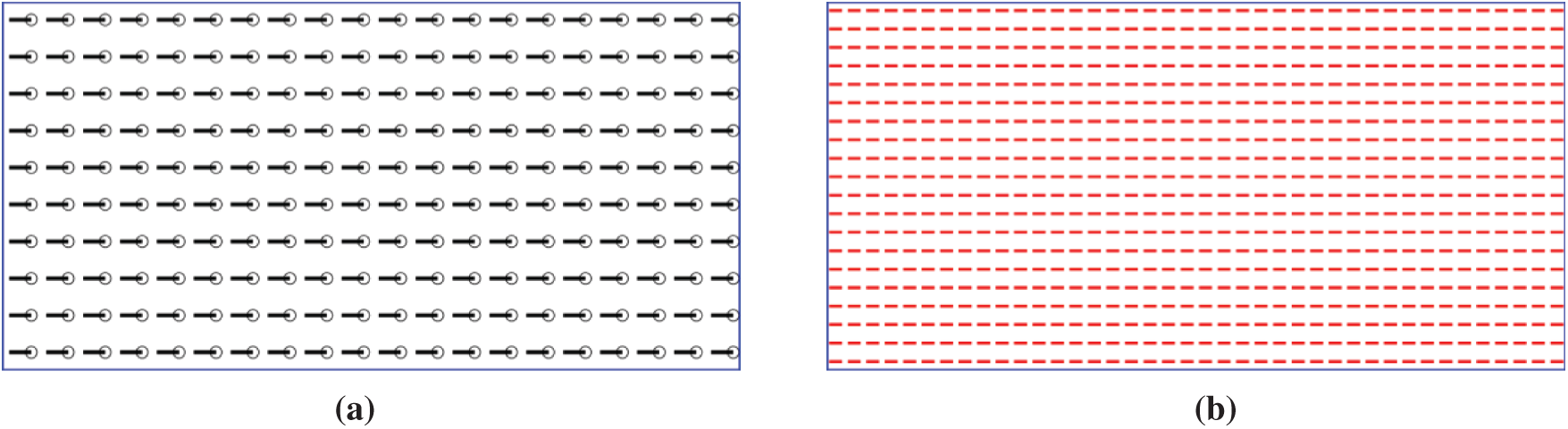
Figure 3: The initial arrangement of fiber angles for the first example. (a) Initial fiber angles at design points, (b) initial fiber angles at center points of finite elements

Figure 4: The results of the first example with

Figure 5: The convergence history of the first example
Next, we investigate the influence of the number of bilateral filtering on the optimization results. We will also analyze the influence of domain filtering parameter
When the number of bilateral filtering in each iteration is investigated, the parameters are set as
Table 1: The optimization results with different numbers of repetitions of bilateral filtering in each iteration (with fixed parameters

Next, the influence of the domain filtering parameter
Table 2: The optimization results obtained with different

Table 3: The optimization results obtained with different

The second design problem is shown in Fig. 6. The design domain is

Figure 6: Design problem of the second example

Figure 7: The initial arrangement of fiber angles for the second example. (a) Initial fiber angles at design points, (b) initial fiber angles at center points of finite elements

Figure 8: The results of the second example with
It can be seen from Fig. 8b that the fiber paths are almost parallel to each other, which means that there exists no gap or overlap between adjacent fiber tows. In addition, the fiber paths are fairly smooth, which means that their curvatures are not large. At the same time, the optimization results also show that the suggested values of the parameters for the bilateral filter in the first example are reasonable.

Figure 9: Design problem of the third example
The third design problem is shown in Fig. 9. The design domain is

Figure 10: The initial arrangement of fiber angles for the third example. (a) Initial fiber angles at design points, (b) initial fiber angles at center points of finite elements

Figure 11: The optimization results of the third example with
In this paper, the bilateral filter was integrated into the Shepard-interpolation-based method for the optimization of composite structures. According to the bilateral filter, sensitivities at design points in the filter area are smoothed by both domain filtering and range filtering. Then, the filtered sensitivities are used to update the design variables. Through several numerical examples, it was found out that the bilateral filter is useful to avoid gap/overlap between adjacent fiber tows or excessive curvature of fiber tows.
Funding Statement: This research work was supported by the National Natural Science Foundation of China (Grant No. 51975227) and the Natural Science Foundation for Distinguished Young Scholars of Hubei Province, China (Grant No. 2017CFA044).
Conflicts of Interest: The authors declare that they have no conflicts of interest to report regarding the present study.
1. Xu, Y. J., Zhu, J. H., Wu, Z., Cao, Y. F., Zhao, Y. B. et al. (2018). A review on the design of laminated composite structures: Constant and variable stiffness design and topology optimization. Advanced Composites and Hybrid Materials, 1(3), 460–477. DOI 10.1007/s42114-018-0032-7. [Google Scholar] [CrossRef]
2. Nikbakt, S., Kamarian, S., Shakeri, M. (2018). A review on optimization of composite structures Part I: Laminated composites. Composite Structures, 195(1), 158–185. DOI 10.1016/j.compstruct.2018.03.063. [Google Scholar] [CrossRef]
3. Ghiasi, H., Pasini, D., Lessard, L. (2009). Optimum stacking sequence design of composite materials Part I: Constant stiffness design. Composite Structures, 90(1), 1–11. DOI 10.1016/j.compstruct.2009.01.006. [Google Scholar] [CrossRef]
4. Ghiasi, H., Fayazbakhsh, K., Pasini, D., Lessard, L. (2010). Optimum stacking sequence design of composite materials Part II: Variable stiffness design. Composite Structures, 93(1), 1–13. DOI 10.1016/j.compstruct.2010.06.001. [Google Scholar] [CrossRef]
5. Dirk, H. L., Ward, C., Potter, K. D. (2012). The engineering aspects of automated prepreg layup: History, present and future. Composites Part B, 43, 997–1009. DOI 10.1016/j.compositesb.2011.12.003. [Google Scholar] [CrossRef]
6. Tatting, B. F., Gürdal, Z., Jegley, D. (2002). Design and manufacture of elastically tailored tow placed plates. [Google Scholar]
7. Wu, K., Tatting, B., Smith, B., Stevens, R., Occhipinti, G. et al. (2009). Design and manufacturing of tow-steered composite shells using fiber placement. 50th AIAA/ASME/ASCE/AHS/ASC Structures, Structural Dynamics, and Materials Conference. California: Palm Springs. [Google Scholar]
8. Brampton, C. J., Wu, K. C., Kim, H. A. (2015). New optimization method for steered fiber composites using the level set method. Structural and Multidisciplinary Optimization, 52(3), 493–505. DOI 10.1007/s00158-015-1256-6. [Google Scholar] [CrossRef]
9. Bruyneel, M., Zein, S. (2013). A modified fast marching method for defining fiber placement trajectories over meshes. Computers and Structures, 125(2), 45–52. DOI 10.1016/j.compstruc.2013.04.015. [Google Scholar] [CrossRef]
10. Lozano, G. G., Tiwari, A., Turner, C., Astwood, S. (2016). A review on design for manufacture of variable stiffness composite laminates. Proceedings of the Institution of Mechanical Engineers, Part B: Journal of Engineering Manufacture, 230(6), 981–992. DOI 10.1177/0954405415600012. [Google Scholar] [CrossRef]
11. Brooks, T. R., Martins, J. R. (2018). On manufacturing constraints for tow-steered composite design optimization. Composite Structures, 204(3), 548–559. DOI 10.1016/j.compstruct.2018.07.100. [Google Scholar] [CrossRef]
12. Hao, P., Liu, D. C., Wang, Y., Liu, X. X., Wang, B. et al. (2019). Design of manufacturable fiber path for variable-stiffness panels based on lamination parameters. Composite Structures, 219(2), 158–169. DOI 10.1016/j.compstruct.2019.03.075. [Google Scholar] [CrossRef]
13. Hong, Z., Peeters, D., Turteltaub, S. (2020). An enhanced curvature-constrained design method for manufacturable variable stiffness composite laminates. Computers and Structures, 238(C), 106284. DOI 10.1016/j.compstruc.2020.106284. [Google Scholar] [CrossRef]
14. Tian, Y., Pu, S. M., Shi, T. L., Xia, Q. (2021). A parametric divergence-free vector field method for the optimization of composite structures with curvilinear fibers. Computer Methods in Applied Mechanics and Engineering, 373(14), 113–574. DOI 10.1016/j.cma.2020.113574. [Google Scholar] [CrossRef]
15. Tian, Y., Pu, S. M., Zong, Z. H., Shi, T. L., Xia, Q. (2019). Optimization of variable stiffness laminates with gap-overlap and curvature constraints. Composite Structures, 230(6), 111–494. DOI 10.1016/j.compstruct.2019.111494. [Google Scholar] [CrossRef]
16. Tian, Y., Huo, Y. H., Shi, T. L., Xia, Q. (2021). Filters for manufacturability in design optimization of variable stiffness composites. Chinese Journal of Aeronautics, 34(4), 153–159. DOI 10.1016/j.cja.2020.07.028. [Google Scholar] [CrossRef]
17. Tian, Y., Mou, J. X., Shi, T. L., Xia, Q. (2019). Shepard interpolation based on geodesic distance for optimization of fiber reinforced composite structures with non-convex shape. Applied Composite Materials, 26(2), 575–590. DOI 10.1007/s10443-018-9731-z. [Google Scholar] [CrossRef]
18. Xia, Q., Shi, T. L. (2018). A cascadic multilevel optimization algorithm for the design of composite structures with curvilinear fiber based on Shepard interpolation. Composite Structures, 188(2014), 209–219. DOI 10.1016/j.compstruct.2018.01.013. [Google Scholar] [CrossRef]
19. Tomasi, C., Manduchi, R. (1998). Bilateral filtering for gray and color images. Proceedings of the 1998 IEEE International Conference on Computer Vision, pp. 839–846. Bombay, India. [Google Scholar]
20. Michael, Y. W., Wang, S. Y. (2005). Bilateral filtering for structural topology optimization. International Journal for Numerical Methods in Engineering, 63(13), 1911–1938. DOI 10.1002/nme.1347. [Google Scholar] [CrossRef]
21. Jiang, W., Baker, M. L., Wu, Q., Bajaj, C., Chiu, W. (2003). Applications of a bilateral denoising filter in biological electron microscopy. Journal of Structural Biology, 144(1), 114–122. DOI 10.1016/j.jsb.2003.09.028. [Google Scholar] [CrossRef]
22. Zhou, M., Rozvany, G. I. N. (1991). The COC algorithm. Part II: Topological, geometrical and generalized shape optimization. Computer Methods in Applied Mechanics and Engineering, 89(1–3), 309–336. DOI 10.1016/0045-7825(91)90046-9. [Google Scholar] [CrossRef]
23. Bendsøe, M. P., Sigmund, O. (1999). Material interpolation schemes in topology optimization. Archive of Applied Mechanics, 69(9–10), 635–654. DOI 10.1007/s004190050248. [Google Scholar] [CrossRef]
24. Kang, Z., Wang, Y. Q. (2012). A nodal variable method of structural topology optimization based on Shepard interpolant. International Journal for Numerical Methods in Engineering, 90(3), 329–342. DOI 10.1002/nme.3321. [Google Scholar] [CrossRef]
25. Kang, Z., Wang, Y. Q. (2011). Structural topology optimization based on non-local Shepard interpolation of density field. Computer Methods in Applied Mechanics and Engineering, 200(49), 3515–3525. DOI 10.1016/j.cma.2011.09.001. [Google Scholar] [CrossRef]
26. Shepard, D. (1968). A two-dimensional interpolation function for irregularly-spaced data. Proceedings of the 23rd National Conference, pp. 517–523. New York, USA: ACM. [Google Scholar]
27. Brodlie, K., Asim, M., Unsworth, K. (2005). Constrained visualization using the Shepard interpolation family. Computer Graphics Forum, 24(4), 809–820. DOI 10.1111/j.1467-8659.2005.00903.x. [Google Scholar] [CrossRef]
28. Lodha, S. K., Franke, R. (1997). Scattered data techniques for surfaces. Scientific Visualization Conference, pp. 189–230. Dagstuhl, Germany. [Google Scholar]
29. Farwig, R. (1986). Rate of convergence of Shepard’s global interpolation formula. American Mathematical Society, 46, 577–590. DOI 10.1090/S0025-5718-1986-0829627-0. [Google Scholar] [CrossRef]
 | This work is licensed under a Creative Commons Attribution 4.0 International License, which permits unrestricted use, distribution, and reproduction in any medium, provided the original work is properly cited. |