Computer Modeling in Engineering & Sciences

DOI: 10.32604/cmes.2021.014477

ARTICLE

Control Charts for the Shape Parameter of Power Function Distribution under Different Classical Estimators

Azam Zaka1, Ahmad Saeed Akhter1, Riffat Jabeen*,2 and Aamir Sanaullah2

1College of Statistical & Actuarial Sciences, University of the Punjab, Lahore, 54000, Pakistan
2COMSATS University Islamabad, Lahore Campus, Lahore, 54000, Pakistan
*Corresponding Author: Riffat Jabeen. Email: drriffatjabeen@cuilahore.edu.pk
Received: 30 September 2020; Accepted: 20 February 2021

1  Introduction

The reliability engineer is very keen on the quality of manufactured products. There is always some variation observed in the output of the process. This variation may be classified as the natural and unnatural cause. Statistical process control (SPC) is helpful in reducing the unnatural causes of the failures of products. In statistical process control, two types of control charts are mainly used to reduce such unnatural causes. One type of control charts is called a memory type control chart, and the second one is memory less control chart. Memory type control charts are exponentially weighted moving averages control chart, and hybrid exponentially weighted moving average control chart. Memory less control chart that is mainly used is the Shewhart control chart. Both types of control charts assume that the distribution of the quality characteristic during the process is normal. A lot of work has done in this regard, such as the EWMA control charts, firstly by Roberts [1] and recently by Li et al. [2] and Nguyen et al. [3]. The cumulative-sum (CUSUM) control chart firstly by Page [4], and recently by [5–7]. The mixed EWMA-CUSUM control charts by [8,9]; and the hybrid exponential weighted moving average (HEWMA) control charts due to Shamma et al. [10], and Haq [11]. All of these are based on the assumption of normality of the process.

In a real life scenario, this is not always possible to fulfil the normality assumption for the distributions of error during the process. A very few work in literature is about this situation including [12–18].

Power function distribution (PFD) has vast application in reliability engineering and survival analysis. To identify and remove the unnatural variation in the process that follows PFD, we will develop control charts to control the process. PFD was introduced by Dallas [19] as the inverse of Pareto distribution. Meniconi et al. [20] showed it as a better fit for reliability data analysis over exponential, Weibull and lognormal distributions.

The core objective of our study is the construction of Shewhart, EWMA and HEWMA control chart by assuming that the distribution of the underlying process follows a Power function distribution. In next section, we have introduced Shewhart, EWMA and HEWMA under normality assumption. In Section 3, we have introduced PFD and provided the estimator of the shape parameter of the PFD. In Section 4, we have proposed the process monitoring for PFD. In Section 5, the steps involved in simulation studies are defined in detail. In Section 6, we have discussed the results obtained by using Section 5. In Section 7, concluding remarks on proposed control charts are given.

2  Some Existing Control Charts When the Assumption of Normality is Assumed

When the distribution of the process is normal, many types of control charts have been constructed in literature. Some of them are:

2.1 Shewhart [21] Control Chart

Suppose that the variable of interest has a normal distribution with mean μ and variance σ2, then control limits for the Shewhart chart is given by

LCL=μ-(L*σ/n)andUCL=μ+(L*σ/n) where “σ” is the standard error of estimate and n is is the sample size. Also, “L” is coefficient which with a standard error of estimate determine in-control average run length.

2.2 Exponentially Weighted Moving Average (EWMA) Control Chart

Let the distribution of the underlying process having the sequence “Yt” is normal. Also, let the 0≤λ1≤1 is a known constant. Now EWMA statistics is given byWt=λ2yt+(1-λ2)Wt-1.

The smoothing constant λ2 plays a very important here. As it approaches zero, it becomes sensitive for small and moderate shifts in mean and close to one. It approaches to Shewart control chart. The control limits for EWMA are given below:

UCLWt=μ+L*V(Wt)LCLWt=μ-L*V(Wt)

2.3 Hybrid Exponentially Weighted Moving Average (HEWMA) Control Chart

Let the distribution of the underlying process having the sequence “Yt” is normal. Also, let the 0≤λi≤1 for i = 1, 2 is a known constant. Now consider a new sequence HEWt as

HEWt=λ1Wt+(1-λ1)HEWt-1(1)

where

Wt=λ2μ^t+(1-λ2)Wt-1(2)

where HEW0=W0=μ and HEWt is a plotting statistics. By placing (2) in (1), we get the following:

HEWt=λ1λ2∑i=0t-1(1-λ1)i∑j=0t-i-1(1-λ11-λ2)jYi+λ1∑i=0t-1(1-λ1)i(1-λ2)t-iμ+(1-λ1)tμ

The mean and variance of HEWt are given below:

E(HEWt)=μV(HEWt)=(λ1λ2(λ1-λ2))2[∑i=12(1-λ1)2(1-(1-λi)2t/1-(1-λi)2)-2(1-λ1)(1-λ2){1-(1-λ1)t(1-λ2)t}1-(1-λ1)(1-λ2)]σ2

The control limits for the HEWMA control chart is explained as

UCLHEWt=μ+L*V(HEWt)LCLHEWt=μ−L*V(HEWt)

3  Power Function Distribution and Estimation of Its Shape Parameters

The PFD is a flexible model for offering a suitable fit for the data related to the failure of components. Dallas [19] introduces it as an inverse of Pareto distribution. Further, Meniconi et al. [20] show that PFD is a better fit for the failure time data over Exponential, Lognormal and Weibull distribution.

The probability density function (pdf) and cumulative density function (cdf) for the PFD are given respectively by

f(y)=γyγ-1βγ;0<y<β

and

F(y)=(yβ)γ,where “β” and “γ” are the scale and shape parameters.

Highly precise estimation of parameters for the distribution of a process is of immense importance as biased estimation may lead to misleading conclusions. In this section, our focus is to estimate the parameters of a PFD using such an estimation method which is more simple and efficient to replace some existing comparatively complex and tedious estimation methods. Zaka et al. [22,23] have shown percentile estimator (P.E), maximum likelihood estimator (MLE), and modified maximum likelihood estimators (MMLE) are more efficient classical estimators for PFD.

3.1 Percentile Estimator (P.E) for the Shape Parameter of PFD

The percentile method is assumed to be first introduced by Dubey [24] for Weibull distribution to estimate the parameters of distribution and proved a better alternative to the MLE. Marks [25] and Zaka et al. [22] have extended the use of P.E to estimate the parameters of a different probability distribution. Zaka et al. [23] derived the P.E for the PFD and observed P.E as equally efficient as MLE, but the difference is the reduction in required constraints for estimating the unknown parameters. However, as the sample size is increased, both methods provide closer estimates of parameters of PFD. It is interesting to mention that P.E uses the two percentile points to estimate the parameters and no recursive equations are required to solve.

The P.E due to Zaka et al. [23] for the shape parameter (γ) is given by

γ^P.E=ln(HL) ln(PHPL)(3)

where “H” and “L” are the maximum and minimum percentile points, different pairs of H and L are used, as 25th, and 75th percentile, 10th and 90th percentile or any other pair of percentile can be used to calculate the shape parameter of PFD. We consider P.E as an unbiased estimator to construct the EWMA control chart. The variance of the “γ^P.E” is defined by

Var(γ^P.E)=E(γ^P.E-γ)2(4)

3.2 MLE for the Shape Parameter of PFD

The MLE due to Zaka et al. [23] for the shape parameter “γ” is given by

γ^MLE=(nnln(max(yi))-∑i=1nlnyi),(5)

where max(yi) is the maximum observation in the data, ln(yi) is the natural logarithm of “yi” and “n” is the sample size.

The variance of the γ^MLE is given by

Var(γ^MLE)=E(γ^MLE-γ)2.(6)

3.3 MMLE for the Shape Parameter of PFD

Zaka et al. [23] proposed the MMLE for the shape parameter of the PFD. The MMLE due to the Zaka et al. [23] for the shape parameter (γ) is given by

γ^ MMLE=−1+(1+(y¯2/S2),(7)

where y¯ and S2 are the sample mean and sample variance, respectively.

The variance of the γ^MMLE is given by

Var(γ^MMLE)=E(γ^MMLE-γ)2.(8)

4  Proposed Process Monitoring For a Power Function Distribution

In the following section, P.E, MLE and MMLE due to Zaka et al. [23] are used to construct memory less and memory-based control charts to monitor the shape parameter of a process follows a PFD.

4.1 Proposed Monitoring of Shape Parameter of PFD Using P.E

Let y1,y2,…,yn be a sequence of independent and identical random variable generated from a process which follows a PFD with shape parameter “γ”. It is important to note that we use the estimator of the shape parameter of the process instead of average of observations or single observations by assuming that E(γ^)=γ.

4.1.1 Shewhart Type Control Chart Using P.E of PFD

The control limits for Shewhart-type control chart using P.E are given by

LCLγ^P.E=γ-L*var(γ^P.E)(9)

CLγ^P.E=γ(10)

UCLγ^P.E=γ+L*var(γ^P.E).(11)

4.1.2 EWMA Control Chart Based on the P.E of PFD

We use the P.E of the shape parameter of the process instead of average of observations or single observations by assuming that E(γ^P.E)=γ.

The EWMA statistic based on P.E of the PFD is given by

PEWt=λγ^P.E+(1-λ)PEWt-1,(12)

where γ^P.E is a P.E as given by (1) for a PFD and PEWt −1 is the statistic on previous time. Also λ is a smoothing constant. The mean and variance are derived as

For t=1 we get,PEW1=λγ^P.E(1)+(1-λ)PEW0,For t=2 we get,PEW2=λγ^P.E(2)+(1-λ)PEW1,PEW2=λγ^P.E(2)+(1-λ)λγ^P.E(1)+(1-λ)2PEW0.

Similarly, on generalizing, we get

PEWt=λγ^P.E(t)+(1-λ)λγ^P.E(t-1)+(1-λ)2γ^P.E(t-2)+…+(1-λ)t-1λγ^P.E(1)+(1-λ)tPEW0,(13)

where PEW0=γ, Taking expectation on, we get

E(PEWt)=λE(γ^P.E(t))+(1-λ)λE(γ^P.E(t-1))+λ(1-λ)2E(γ^P.E(t-2))+…+λ(1-λ)t-1λE(γ^P.E(1))+(1-λ)tPEW0.

We have E(γ^P.E(t))=γ, and PEW0=γ, so the above may be written as

E(PEWt)=λγ+(1-λ)λγ+λ(1-λ)2γ+….+λ(1-λ)t-1λγ+(1-λ)tγ,E(PEWt)=γ[λ{1+(1-λ)+(1-λ)2+…+(1-λ)t-1}+(1-λ)t].

After solving the geometric series, we get

E(PEWt)=γ[λ[1-(1-λ)t1-(1-λ)]+(1-λ)t],

Finally, we get

E(PEWt)=γ.(14)

To get the variance, apply variance on the

Var(PEWt)=λVar(γ^P.E(t))+(1-λ)λVar(γ^P.E(t-1))+λ(1-λ)2Var(γ^P.E(t-2))+…+λ(1-λ)t-1λVar(γ^P.E(1))+(1-λ)tPEW0.

Let Var(γ^P.E(t))=υ=E(γ^P.E-γ)2, we get

Var(PEWt)=λ2υ(1+(1-λ)2+(1-λ)4+…+(1-λ)2(t-1)).

After simplification of a geometric series, we get

Var(PEWt)=λ2υ(1-(1-λ)2t1-(1-λ)2).

Alternatively, we get

Var(PEWt)=υ(1-(1-λ)2t)(λ2-λ).(15)

Hence the control limits of an EWMA based on P.E are given by

LCLPEWt=γ-L*var(γ^P.E)*λ(2-λ)(1-(1-λ)2t)CLPEWt=γUCLPEWt=γ+L*var(γ^P.E)*λ(2-λ)(1-(1-λ)2t).

where 1-(1-λ)2t approaches to unity as “t” get large so after ignoring it, the control limits for EWMA takes the form as given by

LCLPEWt=γ-L*var(γ^P.E)*λ(2-λ)(16)

CLPEWt=γ(17)

UCLPEWt=γ+L*var(γ^P.E)*λ(2-λ).(18)

4.1.3 HEWMA Control Chart Based on P.E of the Shape Parameter of PFD

The HEWMA statistic using P.E of the shape parameter of the PFD is stated by

PHEWt=λ1PEWt+(1-λ1)PHEWt-1(19)

where PEWt is a usual EWMA statistic based on P.E given as

PEWt=λ2γ^P.E+(1-λ2)PEWt-1(20)

and PHEWt −1 is the statistics on previous time. Also λ1 and λ2 are smoothing constant here. The control limits are given for HEMMA control chart using P.E for the shape parameter of the PFD and using (13) we get

PHEWt=λ1(λ2γ^P.E+(1-λ2)∑j=01((1-λ1)(1-λ2))jγ^P.E(t-1)+(1-λ2)2∑j=02((1-λ1)(1-λ2))jγ^P.E(t-2)+(1-λ2)3∑j=03((1-λ1)(1-λ2))jγ^P.E(t-3)+…+(1-λ2)t-1∑j=0t-1((1-λ1)(1-λ2))jγ^P.E(1))+λ1(1-λ2)t∑j=0t((1-λ1)(1-λ2))jγ^P.E(0)+(1-λ2)tPHEt

LCLPHEWt=γ-L*λ1λ2(λ1-λ2)(∑i=12(1-λi)2(1-(1-λi)2t)1-(1-λi)2-2(1-λ1)(1-λ2){1-(1-λ1)t(1-λ2)t}1-(1-λ1)(1-λ2))var(γ^P.E)CLPHEWt=γUCLPHEWt=γ+L*λ1λ2(λ1-λ2)(∑i=12(1-λi)2(1-(1-λi)2t)1-(1-λi)2-2(1-λ1)(1-λ2){1-(1-λ1)t(1-λ2)t}1-(1-λ1)(1-λ2))var(γ^P.E)

4.2 Proposed Monitoring of the Shape Parameter of PFD Using MLE

Let y1,y2,…,yn be a sequence of independent and identical random variable generated from a process which follows a PFD with shape parameter “γ”. It is important to note that we use the estimator of shape parameter of the process instead of average of observations or single observations by assuming that E(γ^)=γ.

4.2.1 Shewhart-Type Control Chart for MLE of PFD

The control limits for Shewhart-type control charts under MLE may be given as

LCLγ^MLE=γ-L*var(γ^MLE)(21)

CLγ^MLE=γ(22)

UCLγ^MLE=γ+L*var(γ^MLE)(23)

4.2.2 EWMA Control Chart for the MLE of PFD

The EWMA statistic by using MLE of PFD may be written asPEWt=λ2γ^MLE+(1-λ2)PEWt-1 where γ^MLE is MLE for PFD and PEWt −1 is the statistic on previous time. Also λ2 is smoothing constant. Using the mean and variance for the EWMA statistics given in (14) and (15). The control limits given below may be obtained PFD as shown below:

LCLPEWt=γ-L*Var(γ^MLE)(λ2-λ)(24)

CLPEWt=γ(25)

UCLPEWt=γ+L*Var(γ^MLE)(λ2-λ)(26)

4.2.3 HEWMA Control Chart for the MLE of the PFD

The HEWMA statistic by using MLE of PFD may be written as

PHEWt=λ1PEWt+(1-λ1)PHEWt-1(27)

where PEWt is a usual EWMA statistic given as

PEWt=λγ^MLE+(1-λ)PEWt-1(28)

where γ^MLE is maximum likelihood estimator for PFD and PEWt −1 is the statistic on previous time. Also λ is smoothing constant, we get the control limits for HEMMA as

LCLPHEWt=γ-L*λ1λ2(λ1-λ2)(∑i=12(1-λi)2(1-(1-λi)2t)1-(1-λi)2-2(1-λ1)(1-λ2){1-(1-λ1)t(1-λ2)t}1-(1-λ1)(1-λ2))*Var(γ^MLE)

CLPHEWt=γ

UCLPHEWt=γ+L*λ1λ2(λ1-λ2)(∑i=12(1-λi)2(1-(1-λi)2t)1-(1-λi)2-2(1-λ1)(1-λ2){1-(1-λ1)t(1-λ2)t}1-(1-λ1)(1-λ2))*Var(γ^MLE)

4.3 Proposed Monitoring of the Shape Parameter of PFD Using MMLE

Let y1,y2,…,yn be a sequence of independent and identical random variable generated from a process which follows a PFD with shape parameter “γ”. It is important to note that we use the estimator of shape parameter of the process instead of average of observations or single observations by assuming that E(γ^)=γ.

4.3.1 Shewhart-Type Control Chart for MMLE of PFD

The control limits for Shewhart control charts under modified maximum likelihood estimator may be given as

LCLγ^MMLE=γ-(L*Var(γ^MMLE))(29)

CLγ^MMLE=γ(30)

UCLγ^MMLE=γ+(L*Var(γ^MMLE))(31)

4.3.2 EWMA Control Chart for the MMLE of PFD

The EWMA statistic by using MMLE of PFD may be written as

PEWt=λ2γ^MMLE+(1-λ2)PEWt-1(32)

where γ^MMLE is MMLE for PFD and PEWt −1 is the statistic on previous time. Also λ2 is smoothing constant. By using the mean and variance for the EWMA statistics given in (14) and (15), the control limits given below may be obtained PFD as given below:

LCLPEWt=γ-L*Var(γ^MMLE)(λ2-λ)(33)

CLPEWt=γ(34)

UCLPEWt=γ+L*Var(γ^MMLE)(λ2-λ)(35)

4.3.3 HEWMA Control Chart for the MMLE of the PFD

The HEWMA statistic by using MMLE of PFD may be written asPHEWt=λ1PEWt+(1-λ1)PHEWt-1 where PEWt is a usual EWMA statistic given asPEWt=λ2γ^MMLE+(1-λ2)PEWt-1 where γ^MLE is maximum likelihood estimator for PFD and PEWt −1 is the statistic on previous time. Also, λ is smoothing constant; we may get the control limits for HEMMA as

LCLPHEWt=γ-L*λ1λ2(λ1-λ2)(∑i=12(1-λi)2(1-(1-λi)2t)1-(1-λi)2-2(1-λ1)(1-λ2){1-(1-λ1)t(1-λ2)t}1-(1-λ1)(1-λ2))*Var(γ^MMLE)CLPHEWt=γUCLPHEWt=γ+L*λ1λ2(λ1-λ2)(∑i=12(1-λi)2(1-(1-λi)2t)1-(1-λi)2-2(1-λ1)(1-λ2){1-(1-λ1)t(1-λ2)t}1-(1-λ1)(1-λ2))*Var(γ^MMLE)

5  Simulation Study

To compare the performance of Shewhart-type, EWMA and HEWMA control charts for monitoring the shape parameter of the PFD, we use the simulation approach to generate Average Run Length (ARL). We use the following algorithm for simulation.

The Monte Carlo Simulation program for the proposed control charts is executed assuming a process is following PFD.

1.    Generate a random sample of size n = 150 on Yt from the PFD with parameters (β,γ)=(1,2).

2.    Compute γ^*t where *=P.E, MLE and MMLE, using (3), (5) and (7).

3.    Repeat Steps 1 and 2 for 5000 times and compute E(γ^*t) and V(γ^*t).

4.    Repeat Step 3 for 5000 times and compute the mean of E(γ^*t) and V(γ^*t).

5.    Compute control limits to construct Shewhart-type control chart based on γ^*t.

6.    Compute ARL value for each Shewhart-type control chart that based on γ^*t given that process is an in-control state.

7.    Now fix ARL0 = 350 for the in-control state of the process and search the suitable value of “L” so that ARL0 for the in-control state of a process is achieved.

8.    Now assume if the process parameter γ is shifted by 0.05 from its true value and compute ARL1. This step is repeated for different shift values 0.10, 0.15, 0.25 & 0.50, and compute ARL1 in each case of shift values.

9.    Plot ARL values against the values of shift that used in Steps 7 & 8.

10.   It is to note that the procedure of Shewhart-type control chart based on γ^*t observe whether the process following the PFD is in-control or out of control. If the process is in-control, go to Step 1. Otherwise, record the Run Length, i.e., the process remained in control before being declared out-of-control.

11.   Repeat this process 5000 times to obtain the ARLs, SDRLs and fractiles.

5.1 Computing Control Chart Based on EWMA Statistics Integrated with P.E, MLE and MMLE, PEW*t for PFD

12.   Repeat Steps 1 and 2 to compute EWMA statistics, PEW * t taking λ=0.6 and PEW * 0 as the target value of the parameter.

13.   Repeat Steps 3 and 4 for 5000 times to compute the mean of E(PEW*t) and V(PEW*t).

14.   Compute control limits for EWMA control charts integrated with PEW * t statistics subject to the process with PFD is an in-control state.

15.   Repeat from Steps 6 to 11.

5.2 Computing Control Chart Based on HEWMA Statistics Integrated with P.E, MLE and MMLE, PHEW*t for PFD

16.   Repeat Steps 1 and 2 to compute HEWMA statistics, HPEW * t taking λ1=0.30, λ2=0.10, and HPEW * 0 as the target value of the parameter.

17.   Repeat Steps 3 and 4 for 5000 times to compute the mean of E(PHEW*t) and V(PHEW*t).

18.   Compute control limits for HEWMA control charts integrated with HPEW * t statistics subject to the process with PFD is an in-control state.

19.   Repeat from Steps 6 to 11.

20.   Assume λ1=0.30, λ2=0.50 and repeat from Steps 17 to 19.

21.   Assume λ1=0.30, λ2=0.75, and repeat from Steps 17 to 19.

6  Results and Discussion

Average Run length is considered for comparison in between the control charts based on MLE, MMLE and P.E. The timely detection of an outlier in the process is preferred. So the control chart having a minimum ARL value is considered to be good.

We have constructed three control charts, i.e., Shewhart control chart based on P.E, Shewhart control chart based on MLE and Shewhart control chart based on MMLE. We compare these control charts by using the above mentioned simulation steps. We have presented the ARLs by setting the ARLo=500.

We observe from Tab. 1 and Fig. 1 that the performance of a Shewhart control chart based on MLE is better than P.E and MMLE. We see that the MLE early detects the shift in the process. For instance the control chart based on the estimate of shape parameter using P.E gives ARL1, i.e., out of control average run length as 419.257 when there is shift of 0.01 in the shape parameter PFD but MLE gives ARL1 = 392.25 and MMLE gives ARL1 = 430.103. So, MLE is more efficient to detect the small shift in the process compared to P.E and MMLE if the underlying distribution of the process is PFD.

We observe from Tab. 2 and Fig. 2 that for λ=0.10, MLE performs better as compare to P.E and MMLE. We take a shift of 0.01 in the shape parameter of PFD and see that control charts under P.E provide ARL1 = 356.138, control charts under MLE gives ARL1 = 287.2285 and control charts under MMLE gives ARL1 = 307.261. We see that a control chart under MLE is better than control charts under P.E and MMLE. We take different shifts and observe the same behaviour. We observe that the ARL1 reduces to 1 more efficiently when we use EWMA control chart under MLE as compare to the control chart under P.E and control chart under MMLE.

Table 1: Shewhart control chart based on P.E, MLE and MMLE

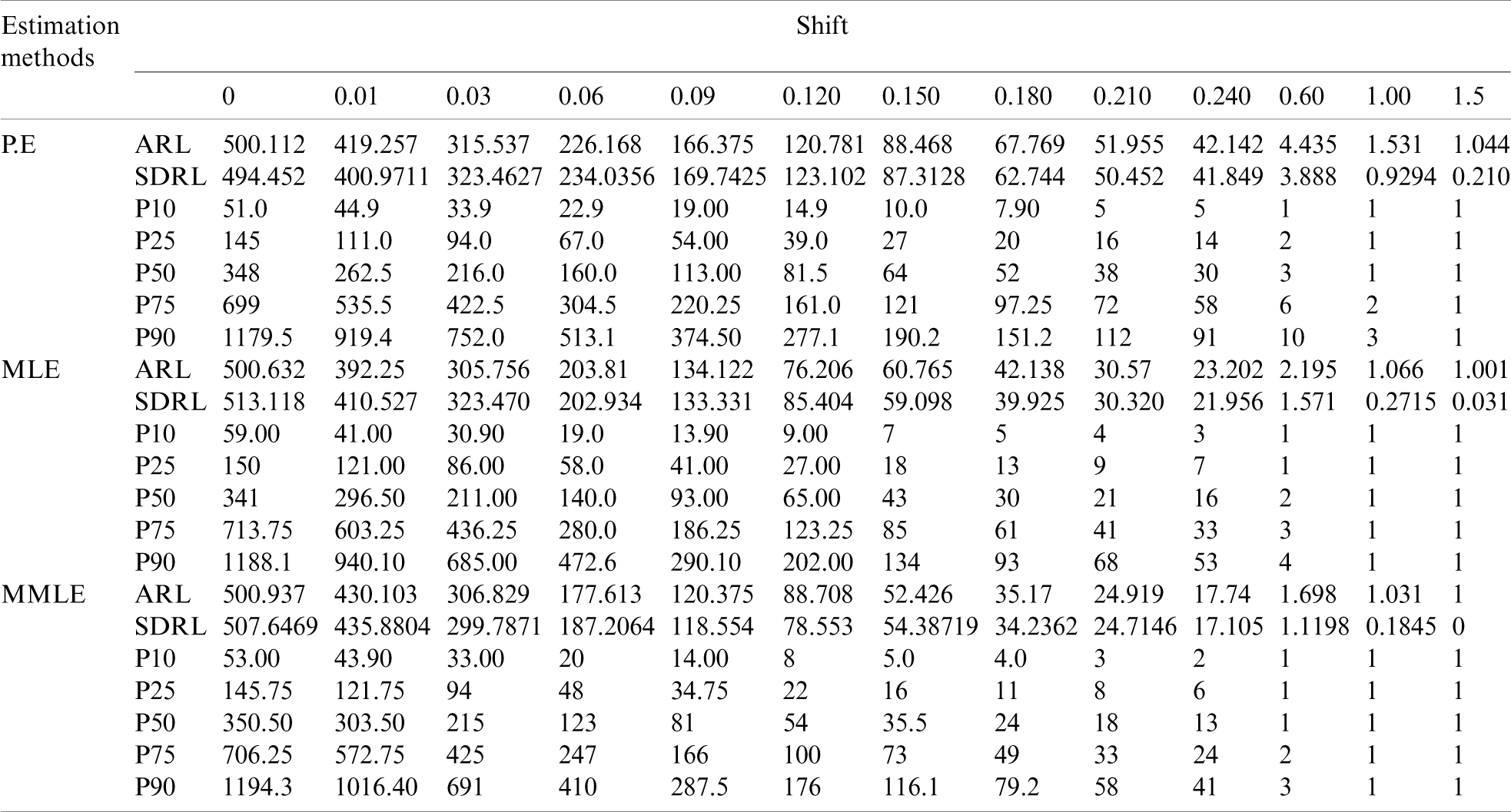
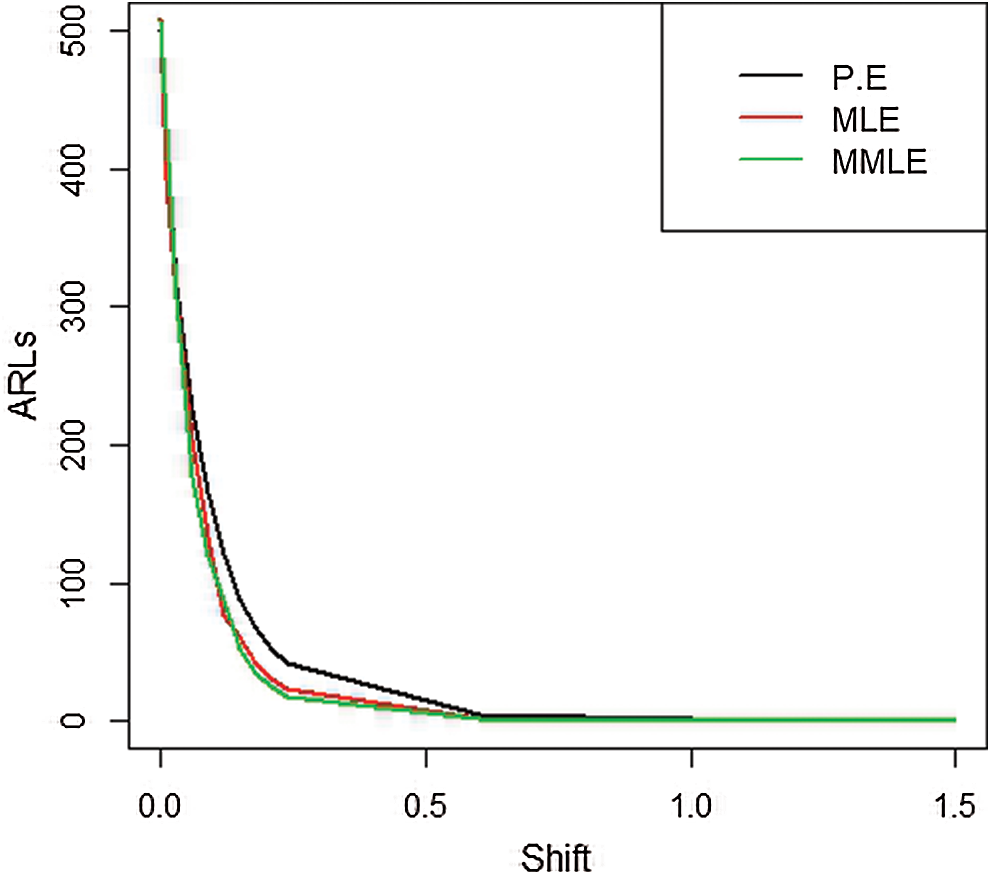
Figure 1: ARLs for the shape parameter of PFD under Shewhart control chart

Table 2: EWMA control chart when λ=0.10 based on P.E, MLE and MMLE for power function distribution

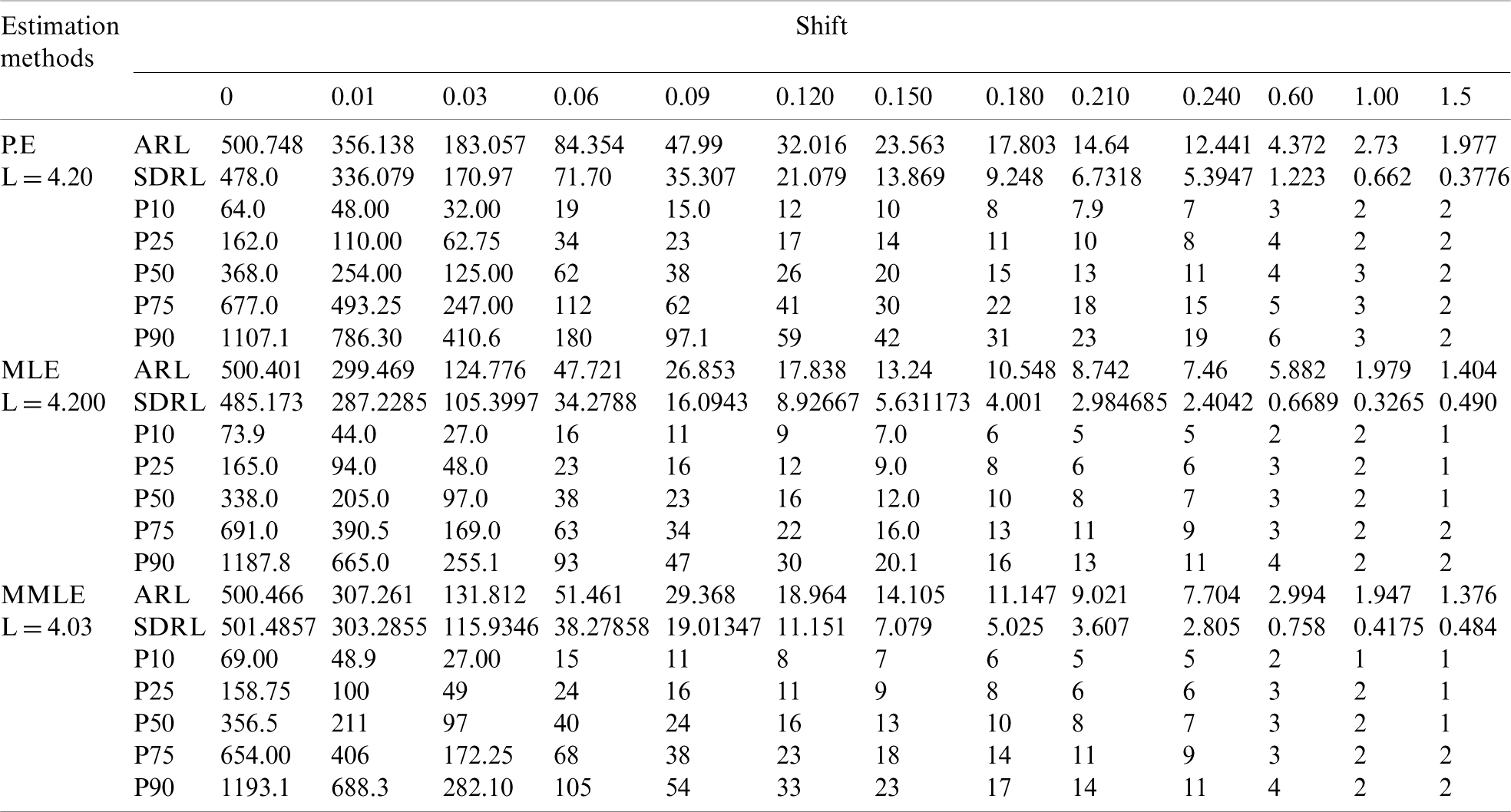
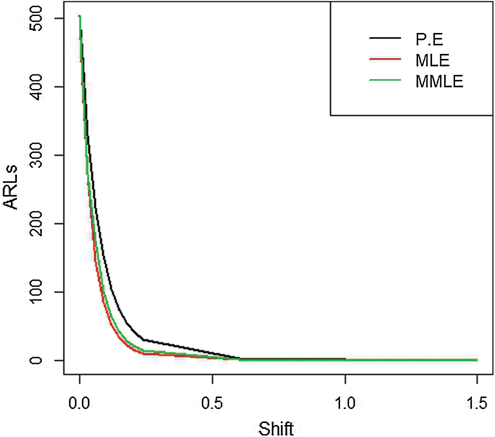
Figure 2: ARLs for the shape parameter of PFD under EWMA control chart at λ=0.75

Table 3: EWMA control chart when λ=0.60 based on P.E, MLE and MMLE for power function distribution

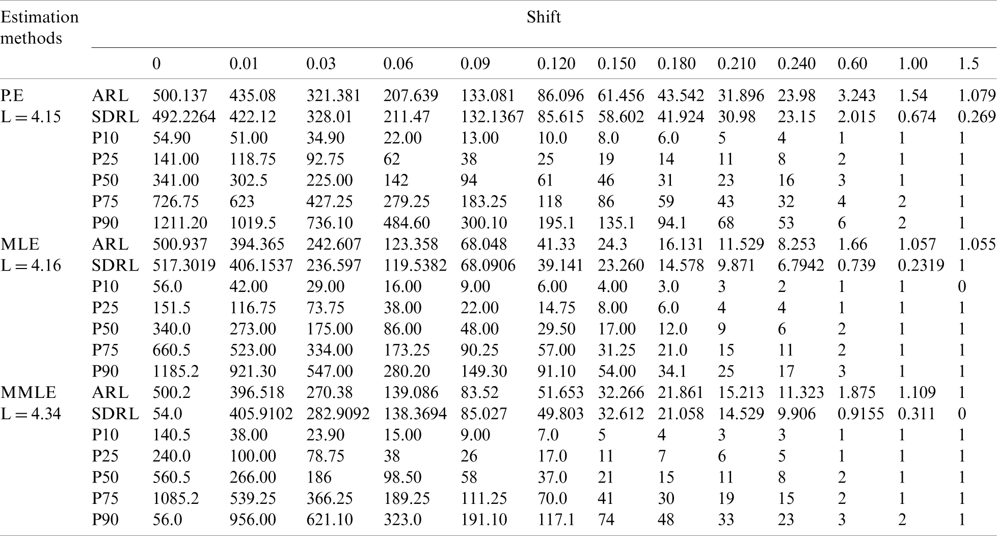
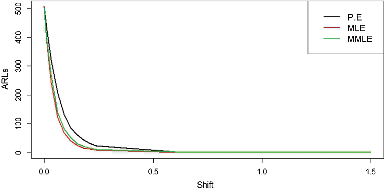
Figure 3: ARLs for the shape parameter of PFD under EWMA control chart at λ=0.60

From Tab. 3 and Fig. 3, it is clear that for λ=0.60, at shift=0.01, P.E provides ARL1 = 435.08, control charts under MLE give ARL1 = 394.365 and control charts under MMLE gives ARL1 = 396.261. We conclude that a control chart under MLE is better than control charts under P.E and MMLE. We also see that if we use different shifts for shape parameter, EWMA under MLE detects early any shift to shape parameter as compare to EWMA under P.E and MMLE.

We can see in Tab. 4 and Fig. 4 that when λ=0.75, by using shift=0.01, EWMA control charts under P.E provide ARL1 = 444.335, control charts under MLE gives ARL1 = 403.633 and control charts under MMLE gives ARL1 = 407.456. We conclude that EWMA control chart under MLE is better than the control charts under P.E and MMLE.

Table 4: EWMA control chart when λ=0.75 based on P.E, MLE and MMLE for power function distribution

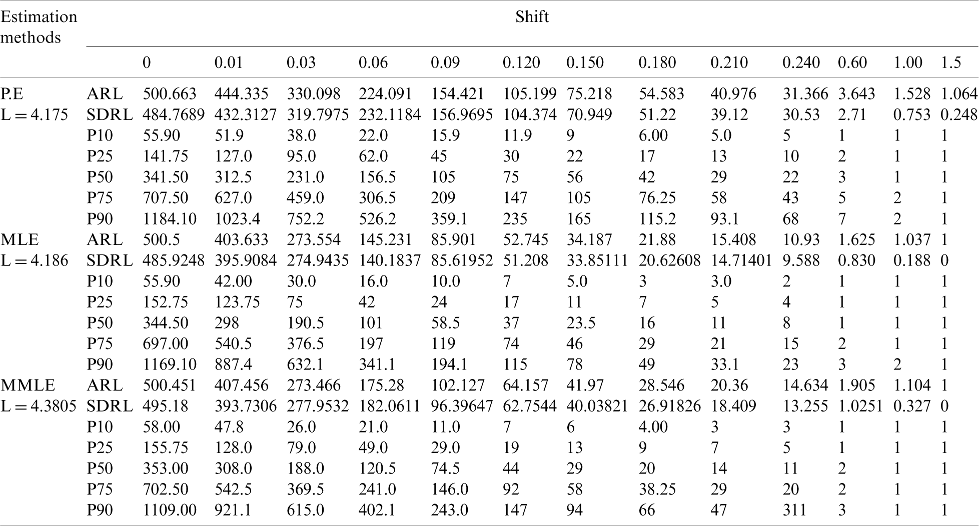
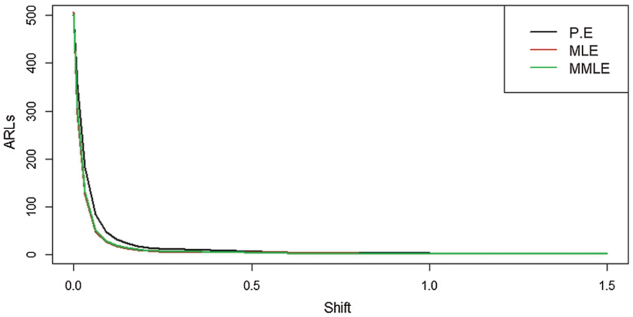
Figure 4: ARLs for the shape parameter of PFD under EWMA control chart at λ=0.10

Table 5: HEWMA control chart when λ1=0.30, λ2=0.10 based on P.E, MLE and MMLE for power function distribution

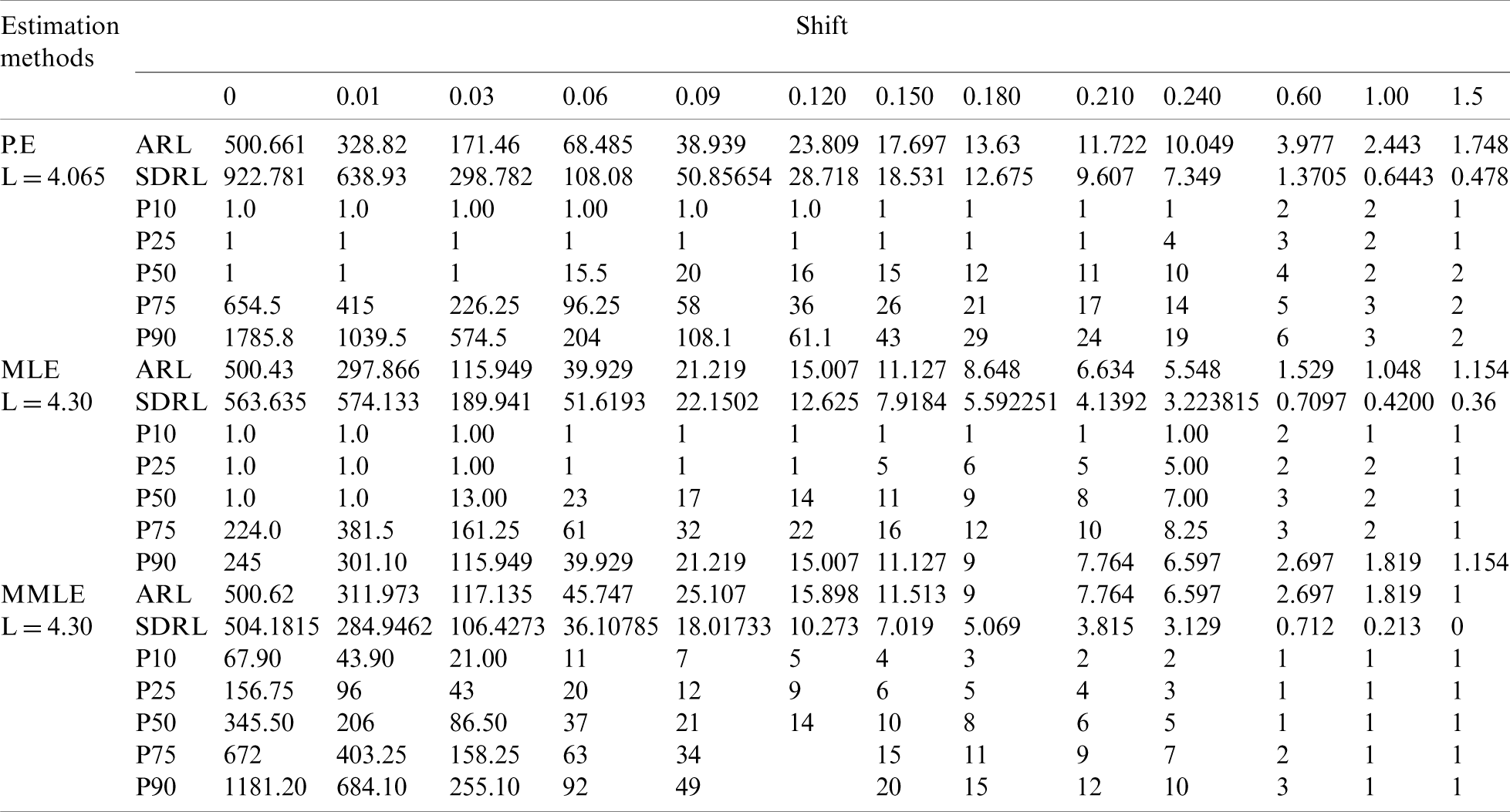
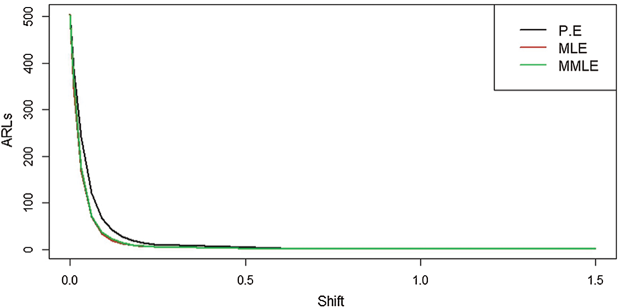
Figure 5: ARLs for the shape parameter of PFD under HEWMA control chart at λ1= 0.30 and λ2= 0.60

Table 6: HEWMA control chart when λ1=0.30, λ2=0.60 based on P.E, MLE and MMLE for power function distribution

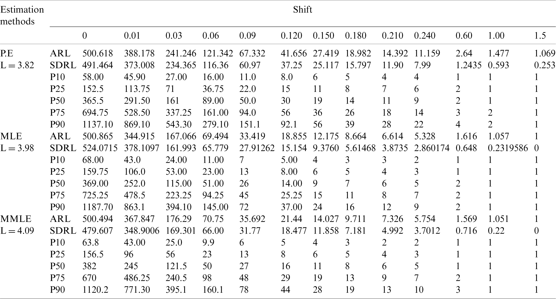
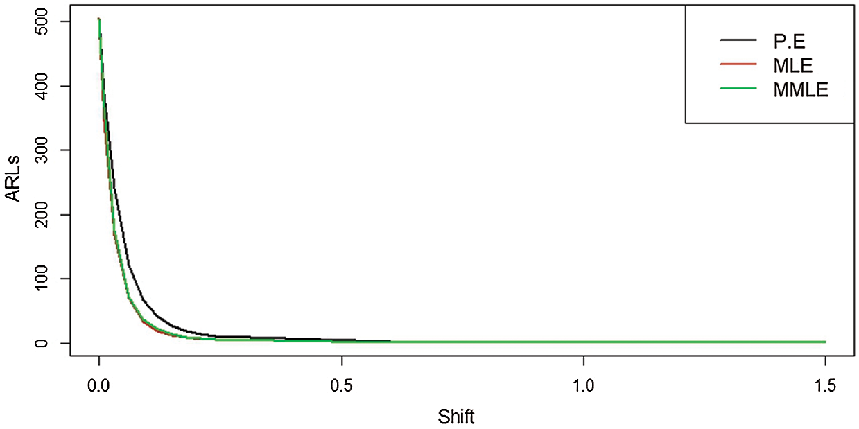
Figure 6: ARLs for the shape parameter of PFD under HEWMA control chart at λ1=0.30 and λ2=0.10

We also observe from Tabs. 1–4 that with an increase in the value of λ, the EWMA control charts behave like Shewhart control chart showing an increase in ARL1. So EWMA performs better than Shewhart control chart for all three control charts based on P.E, MLE and MMLE.

We have developed HEWMA control chart based on P.E, MLE and MMLE when λ1=0.30 and λ2=0.10 in Tab. 5 and Fig. 5. We can see from Tab. 5 that MLE performs better as compare to control charts based on P.E and MMLE when the underlying distribution of the process is PFD. We see that for a shift of 0.01 in the shape parameter of an underlying process, the control chart based on P.E gives ARL1 = 328.82, the control chart based on MLE provide ARL1 = 297.866 and the control chart based on MMLE detects the shift at ARL1 = 311.973. By further analysis of the results given in Tab. 5, we observe the same behaviour of HEWMA under MLE as it gives smaller ARL1 as compare to HEWMA under P.E and MMLE.

From Tab. 6 and Fig. 6, we observe that shift of 0.01 in the shape parameter of an underlying process, the control chart based on P.E detects the shift by giving ARL1 = 388.178), the control chart based on MLE detects the shift ARL1 = 344.91, and the control chart based on MMLE detects the shift at ARL1 = 367.847. From Tab. 7 and Fig. 7, at shift=0.01, the control chart based on P.E detects the shift and gives ARL1 = 390.57, the control chart based on MLE gives ARL1 = 358.786, and the control chart based on MMLE detects the shift at ARL1 = 373.21.

We also observe that HEWMA control chart performs better as compare to EWMA control chart and Shewhart control chart under all three estimation methods, i.e., P.E, MLE and MMLE by giving less ARL1 value, which means early detection of any shift in the process.

6.1 Simulated Data Set

To see the working procedure of the proposed control charts, a simulation study was carried out. For this purpose, we generated 25 observations from a PFD for an in-control process, and the next 25 observations were generated from the shifted process with λ=0.10. The estimated values of the proposed EWMA statistic under MLE were computed for the selected levels of the proposed control charts parameters with λ=0.10 and L=4.20. The data and values of the proposed and existing statistic are listed in Tab. 8, and the plotted values of these statistics are shown in Fig. 8. Further, the estimated values of the proposed HEWMA statistic under MLE were computed for the selected levels of the proposed control charts parameters with λ1=0.30, λ2=0.10 and L = 4.065. The data and values of the proposed and existing statistic are listed in Tab. 8, and the plotted values of these statistics are shown in Fig. 9.

Table 7: HEWMA control chart when λ1=0.30, λ2=0.75 based on P.E, MLE and MMLE for power function distribution

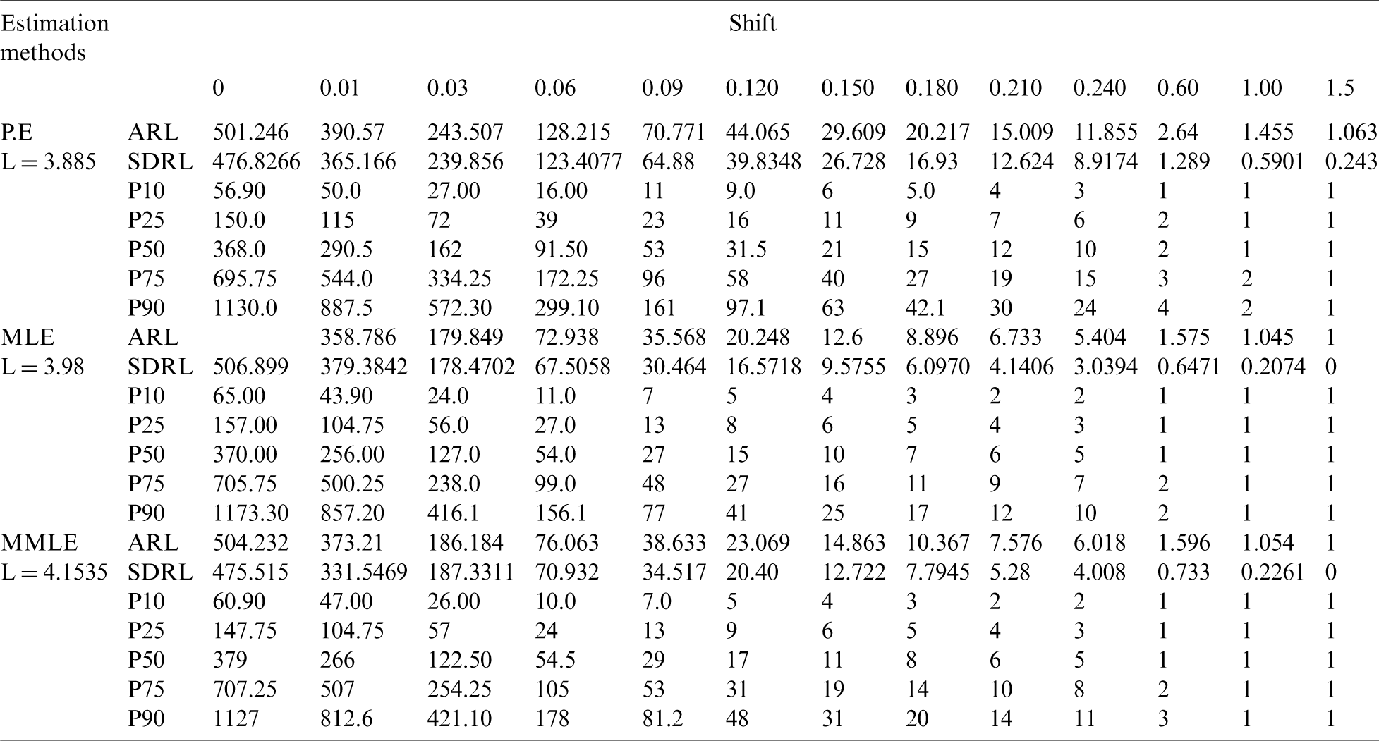
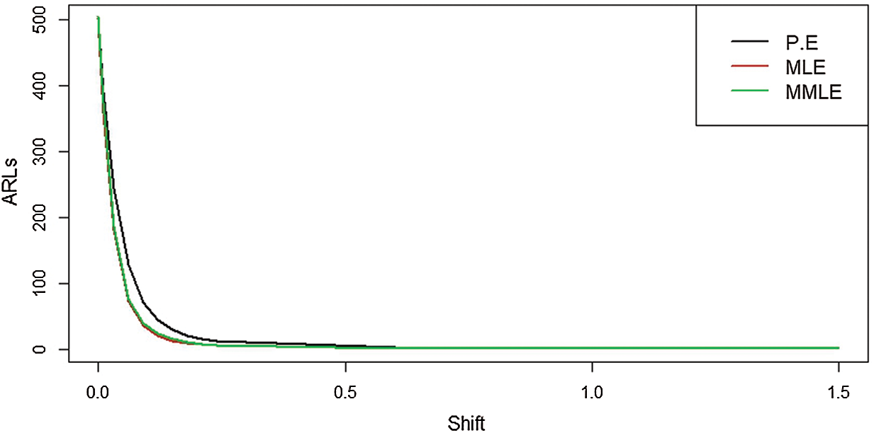
Figure 7: ARLs for the shape parameter of PFD under HEWMA control chart at λ1=0.30 and λ2=0.75

Table 8: Simulated data

In Fig. 9, we noted that the proposed HEWMA control chart under MLE detected a shift at the 32th sample, while in Fig. 8; the EWMA control chart under MLE could not detect the shift. Hence, this shows that the proposed HEWMA control chart under MLE has a greater ability to detect smaller shifts earlier than the EWMA control chart.

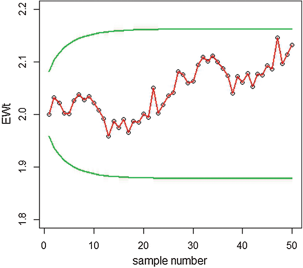
Figure 8: Graph of simulated data of the proposed EWMA control chart under MLE

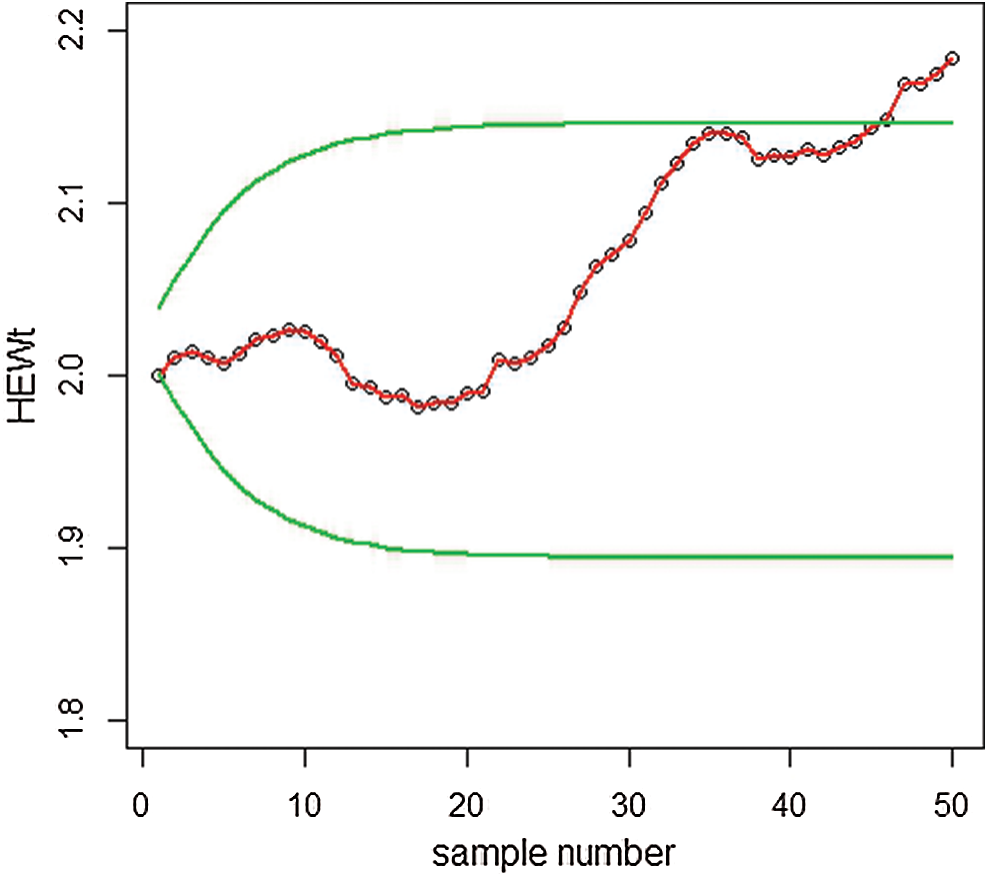
Figure 9: Graph of simulated data of the proposed HEWMA control chart under MLE

6.2 Real Life Application

The data set is reported by Bekker et al. [26], which corresponds to the survival times (in years) of a group of patients given chemotherapy treatment alone. The data consisting of survival times (in years) for 46 patients are: 0.047, 0.115, 0.121, 0.132, 0.164, 0.197, 0.203, 0.260, 0.282, 0.296, 0.334, 0.395, 0.458, 0.466, 0.501, 0.507, 0.529, 0.534, 0.540, 0.641, 0.644, 0.696, 0.841, 0.863, 1.099, 1.219, 1.271, 1.326, 1.447, 1.485, 1.553, 1.581, 1.589, 2.178, 2.343, 2.416, 2.444, 2.825, 2.830, 3.578, 3.658, 3.743, 3.978, 4.003, 4.033. The data follows the PFD and plotted for both EWMA and HEWMA control charts under MLE, as shown in Figs. 10 and 11.

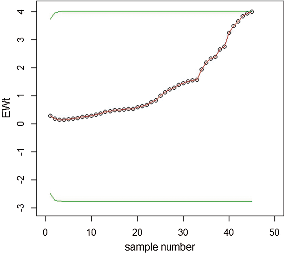
Figure 10: Graph of real data of the EWMA control chart under MLE when L=4.20 and λ=0.10

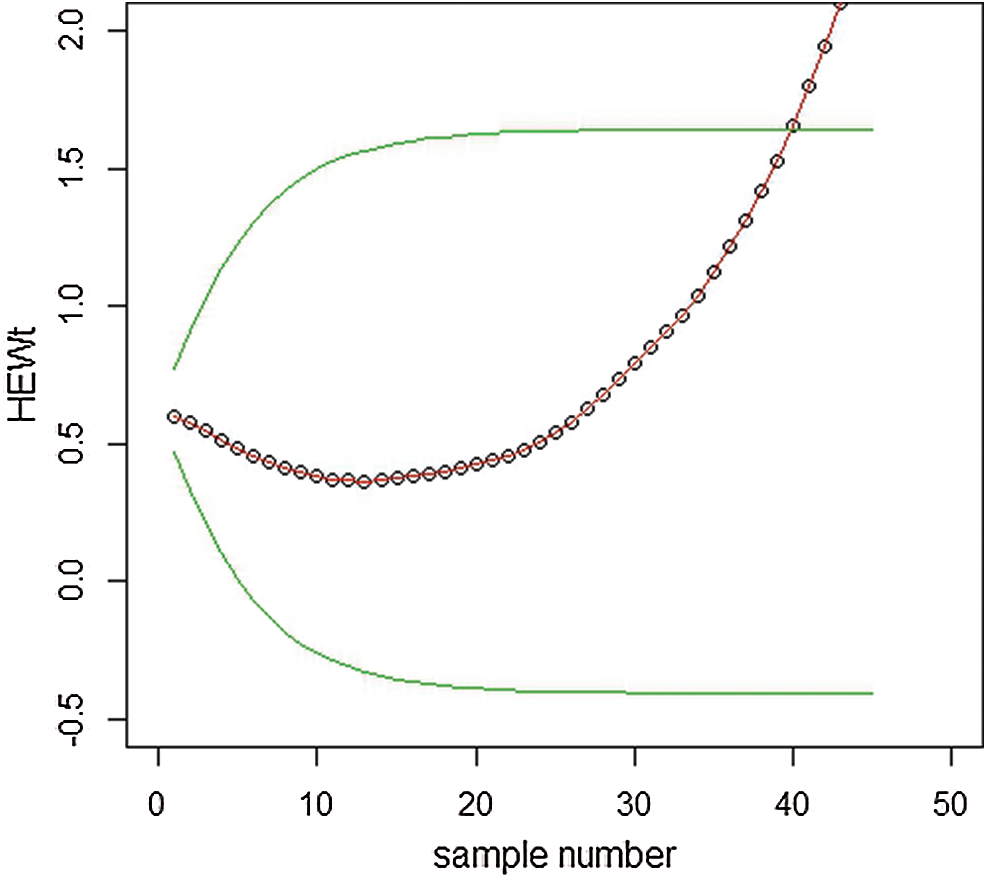
Figure 11: Graph of real data of the HEWMA control chart under MLE when λ1=0.30, λ2=0.10 and L=4.30

We have constructed EWMA for λ=0.10 and HEWMA for λ1=0.30, λ2=0.10 control charts under MLE in Figs. 10 and 11. We see that HEWMA detects the process shift early compared to EWMA, which shows that HEWMA is better to be used in real life when the distribution of the underlying process is PFD.

7  Conclusion

If the process characteristic follows power function distribution, the construction of the usual control charts such as Shewhart control chart, EWMA control chart and HEWMA control chart by assuming the assumption of normality may increase the chances of the use of inappropriate chart which leads to the wrong detection of real changes in the process, to overcome such issue, we have constructed the Shewhart, EWMA and HEWMA control charts by assuming that the distribution of the process is power function distribution. We have used three different estimation methods for the shape parameter of PFD to construct the said control charts. We have concluded that the HEWMA control chart under MLE performs better as compared to the other control charts.

We have used the EWMA and HEWMA control chart under MLE to simulate data and constructed the control charts; We observe that HEWMA under MLE is better to be used for monitoring the process shape parameter. We have also provided the real-life application of the proposed control charts. We observe that when the distribution of process follows PFD, HEWMA control chart under MLE is preferred to be used.

Funding Statement: The authors received no specific funding for this study.

Conflicts of Interest: The authors declare that they have no conflicts of interest to report regarding the present study.

This work is licensed under a Creative Commons Attribution 4.0 International License, which permits unrestricted use, distribution, and reproduction in any medium, provided the original work is properly cited.