| Computer Modeling in Engineering & Sciences |
DOI: 10.32604/cmes.2021.016775
ARTICLE
Monte Carlo Simulation of Fractures Using Isogeometric Boundary Element Methods Based on POD-RBF
1Key Laboratory of In-Situ Property-Improving Mining of Ministry of Education, Taiyuan University of Technology, Taiyuan, 030024, China
2School of Architecture and Civil Engineering, Huanghuai University, Zhumadian, 463003, China
3College of Architecture and Civil Engineering, Xinyang Normal University, Xinyang, 464000, China
4Artificial Intelligence Research Center, National Innovation Institute of Defense Technology, Beijing, 100071, China
5Department of Mechanical Engineering, Suzhou University of Science and Technology, Suzhou, 215009, China
*Corresponding Author: Zhongwang Wang. Email: wangzw9620@163.com
Received: 25 March 2021; Accepted: 22 April 2021
Abstract: This paper presents a novel framework for stochastic analysis of linear elastic fracture problems. Monte Carlo simulation (MCs) is adopted to address the multi-dimensional uncertainties, whose computation cost is reduced by combination of Proper Orthogonal Decomposition (POD) and the Radial Basis Function (RBF). In order to avoid re-meshing and retain the geometric exactness, isogeometric boundary element method (IGABEM) is employed for simulation, in which the Non-Uniform Rational B-splines (NURBS) are employed for representing the crack surfaces and discretizing dual boundary integral equations. The stress intensity factors (SIFs) are extracted by M integral method. The numerical examples simulate several cracked structures with various uncertain parameters such as load effects, materials, geometric dimensions, and the results are verified by comparison with the analytical solutions.
Keywords: Monte Carlo simulation; POD; RBF; isogeometric boundary element method; fracture
Uncertainties are ubiquitous in engineering applications that may arise from different sources such as inherent material randomness, geometric dimensions, manufacturing errors, and dynamic loading. Because deterministic analysis fails to characterize randomness field, stochastic analysis techniques have been extensively studied to strengthen the credibility of computational prediction of uncertainty problems [1]. There are three main variants of stochastic analysis: perturbation based techniques [2], stochastic spectral approaches [3,4], and Monte Carlo simulation (MCs) [5–7]. Among them, the MCs is regarded as the most versatile and simplest approach, and often used as the reference solution to verify the results of Perturbation method and Spectral method, but the exhaustive sampling in MCs leads to a heavy computational burden arising from both solving physical problems and constructing analysis-suitable geometric models that must be addressed carefully.
Combining Proper Orthogonal Decomposition (POD) and Radial Basis Functions (RBF) [8–11] is an effective technique of model order reduction [12–14]. The POD represents the solution field with the special ordered orthogonal functions in a low-dimensional subspace, which is constructed based on a discrete number of system responses obtained from the evaluation of the full order models (FOM) [15]. POD reduces the degrees of freedom by capturing the dominant components of high-dimensional processes because it offers the optimal basis in the sense that the approximation error is minimal in L2 norm. On the other hand, the RBF builds a surrogate model through interpolating the data in the reduced space, whereby it admits continuous approximation of system responses for any arbitrary combination of input parameters [16] and thus does not need to solve partial differential equation for each sample.
The pre-processing time of MCs in constructing geometric models can be reduced with isogeometric analysis (IGA) [17]. The key idea of IGA is employing spline functions used to construct geometric models in Computer Aided Design (CAD), for example Non-Uniform Rational B-splines (NURBS), T-splines [18], PHT-splines [19,20], and subdivision surfaces [21], as the basis functions to discretize physical fields. Compared to traditional Lagrange polynomial based methods, the main advantage of IGA lies in its ability of integrating numerical analysis and CAD. IGA enables one to perform numerical analysis directly from CAD models without meshing, which is particularly beneficial to uncertainty qualification since it requires fast generation of a large number of models. IGA also offers the benefits of geometric exactness, flexible refinement scheme and high order continuity that are amenable to numerical analysis.
Fracture mechanics is crucial in structural integrity assessment and damage tolerance analyses, but simulation of fracture behaviors poses significant challenges to Finite Element Methods (FEM) for the following reasons: (1) the mesh in proximity to cracks should be several orders of magnitude finer than that used for stress analysis; (2) a remeshing procedure is inevitable when cracks extend; (3) stress singularity or high stress gradients need to be captured. The extended finite element method (XFEM) incorporates enrichment functions to solution space and thus allows for crack propagation in a fixed mesh, but it still relies on a fine and good-quality mesh and necessitates special techniques to represent crack surfaces like Level Set Method. In comparison, Boundary Element Method (BEM) [22–26] has proven a useful tool for fracture simulation. Since BEM only discretizes the boundary of the domain, it not only reduces the degrees of freedom and facilities mesh generation, but more importantly, extends the crack by simply adding new elements at the front of cracks. In addition, as a semi-analytical method, BEM evaluates stress more accurately which is critical in extracting stress intensity factors. Furthermore, isogeometric analysis within the context of boundary element method (IGABEM) inherits the advantage of IGA in integration of CAD and numerical analysis and that of BEM in dimension reduction. IGA with BEM is also natural because both of them are boundary-represented. Since its inception, IGABEM has been successfully applied to potential [27–31], linear elasticity [32–36], acoustics [37–44], electromagnetics [45], structural optimization [40,46–49], etc., Peng et al. [50,51] applied IGABEM to two dimensional and three dimensional linear elasticity fracture mechanics, and demonstrates the accuracy and efficiency of IGABEM in this area.
This paper presents a novel procedure for solving uncertainty problems of fracture mechanics. In this method, the IGABEM is employed for fracture analysis, and MCs for addressing multiple random parameters. The computational cost is reduced by combination of POD and RBF. The remaining of this paper is structured as follows. Section 2 introduces the fundamentals of MCs in stochastic analysis. Section 3 illustrates how to apply POD and RBF to MCs. Section 4 formulates IGABEM in linear elasticity fracture mechanics. Several numerical examples are given in Section 5 to test the reliability, accuracy and efficiency of the proposed method, followed by conclusions in Section 6.
2 Stochastic Analysis with Monte Carlo Simulation
Monte Carlo simulation (MCs) directly characterizes uncertainties by calculating expectations and variances from a large number of samples. For a random variable X associated with the probability density function p(x), the two probabilistic moments are defined as
where E[X] is the expectation of the random variable X, and
According to the law of large numbers, the average of the results obtained from a number of samples should converge to the expectation as more sampling points are selected, which is the theoretical basis of MCs. Suppose g(X) is an arbitrary function of the random variable X. The expectation and variance of
where N is the sample size, and the order of convergence rate is O(N−1/2).
MCs in structural analysis can be conducted in the following steps [15]: (1) Identify the random variables that are the source of the uncertainties in the system. (2) Determine the probability density functions of the random variables. (3) Use a random number generator to produce a set of samples which are adopted as the input parameters. (4) Employ a numerical method in deterministic analysis to evaluate the solution for each sample. (5) Based on the outputs of numerical analysis for all of the samples, we calculate the expectation and variance of the system using Eqs. (2) and (3) [52]. From the above, it can be seen that MCs is easy to implement because the existing numerical simulation codes can be directly used without modification. In addition, MCs is versatile and is suitable for complex uncertainty problems. However, Step 3 of MCs is very time consuming because the numerical simulation needs to be conducted as many times as the number of sampling points. The large sample size can enhance the accuracy but may lead to higher computational cost.
3 Proper Orthogonal Decomposition (POD) and Radial Basis Functions (RBF)
As mentioned above, MCs is prohibitively expensive because it needs to solve the physical problems at many samples. This procedure can be accelerated by the reduced-order moeling based on POD and RBF. Let
where
where
By defining
where
Eq. (6) only approximates a discrete number of system responses that are already computed using the FOM. To achieve a continuous approximation of system responses for any arbitrary input parameters, the radial basis functions (RBF) are used to interpolate the amplitudes in the reduced subspace
where N is the number of samples,
in which the symbol
By letting
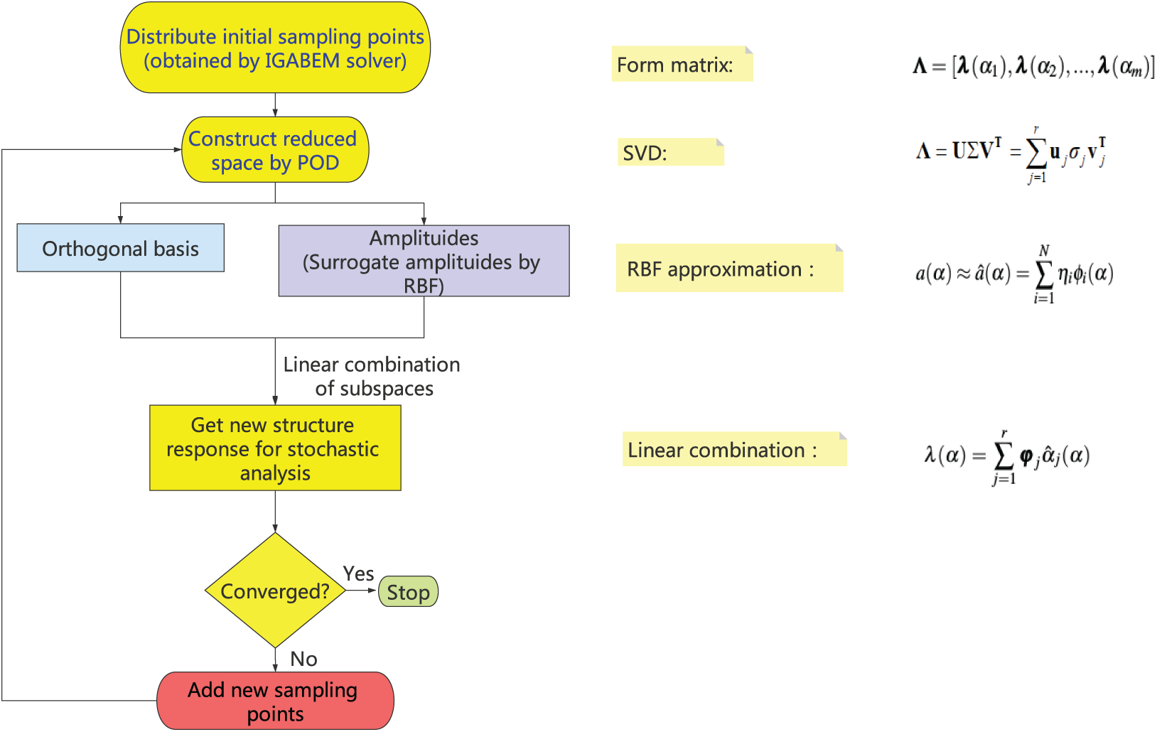
Figure 1: Th flow chart
Hence, the system response for any sample of the stochastic variable can be obtained straightforwardly by Eq. (9) without needing to solve the partial differential equations repeatedly. The algorithm mentioned above is illustrated in the Fig. 1. The POD-RBF enable us to conduct MCs without needing to perform FOM simulation for all of the sample points. However, the FOM is still essential for getting snapshots which is solved by IGABEM in our work as detailed in the following section. Therefore, the number of the samples or snapshots should be selected carefully to strike a balance between the accuracy and efficiency. In the future, we will introduce error estimation technique to improve the performance of our method. In addition, it is highlighted that in order to further enhance the computational efficiency, the number of basis functions in Eqs. (5) and (9) can be decreased by selecting the basis functions corresponding to the elements with larger values in
4 Fracture Modeling with IGABEM
4.1 Boundary Integral Equations in Fracture Mechanics
Consider an arbitrary domain
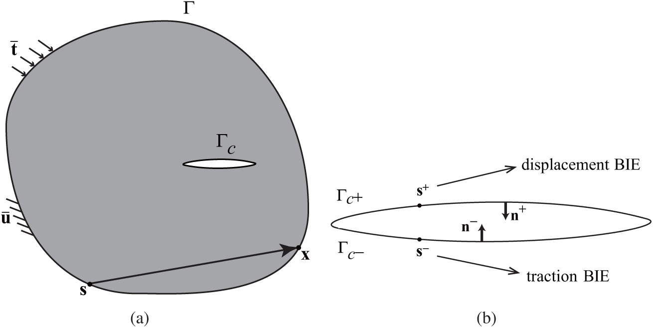
Figure 2: A crack model (a) a cracked elastic body; (b) crack surfaces
Because the crack upper surfaces and lower surfaces are geometrically overlapping, the source points on the two surfaces will coincide and thus the boundary integral equations (BIE) corresponding to them are identical to each other, which leads to the degradation of the system matrix. An effective approach—dual boundary element method (DBEM) [53] can overcome this difficulty by using the traction BIE on one of the crack surface (
where
4.2 IGABEM for Fracture Mechanics
As a powerful geometric modeling technique, NURBS is the industrial standard of CAD and also central to isogeometric analysis. Given a knot vector
where n denotes the order of basis functions and
where
where
In IGABEM, NURBS are used not only for building geometries but also discretizing the boundary integral equations. Hence, the displacement and traction around the boundary can be expressed piecewisely as a linear combination of the NURBS basis function and the nodal parameters,
where
By substituting Eq. (15) into the boundary integral equation (10), we can get the following discretization formulation of Eq. (10)
where
The boundary element method involves weakly singular, strongly singular and hyper singular integrals, which have to be addressed carefully. For this purpose, the subtraction of singularity technique is used, whose implementation details can be seen in [50]. After solving the governing linear equations of IGABEM, we can obtain the displacement and traction field around the boundary. Then, we are able to evaluate the stress intensity factors (SIFs) with M integral [54] and predict the crack propagation direction with maximum hoop stress criterion [55]. See Appendix B for details.
In the following examples, the input random variables are supposed to follow the Gaussian distribution with the expectation being 0.5 and the standard deviation being 0.033. The sampling method for Gaussian distribution function used in this paper is to select sample points in the interval
5.1 Inclined Center Crack Problem
A plate model with an inclined center crack under remote biaxial tension is considered in this section, as shown in Fig. 3. The crack inclination angle is
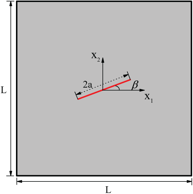
Figure 3: Structural model for an inclined center crack problem
The number of NURBS elements on the initial crack surface is set as 3, and the total DOFs is 86. We fix the crack angle
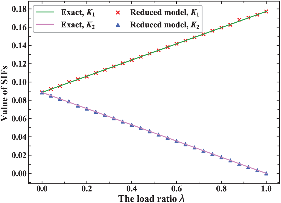
Figure 4: The variation of SIFs with the load ratio
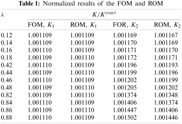
Tab. 1 lists the normalized values of SIFs (the values divided by the exact solution) calculated by the FOM with IGABEM and that by the ROM with POD-RBF. The normalized value of K1 changes slightly with the increase of
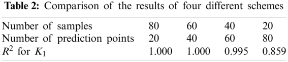
To investigate the influence of the sample size on the accuracy of ROM, we construct a vector,
where n is the total number of the predication points, the subscript i the i-th prediction point, yi the numerical value of the SIF,
Next, we conduct MCs to evaluate the expectation and standard deviation of stress intensity factors. The following three different schemes are adopted for comparison.
1. Stochastic fracture analysis with MCs using FOM is conducted based on 51 samples of
2. We build the ROM with 10, 20, 30, and 40 samples, respectively, and then perform MCs using the 51 samples. In this case, the dimension of the matrix
3. Similar to Case 2, the MCs is performed with the ROM that is established with 10, 20, 30 and 40 samples, respectively. However, we will further decrease the number of the reduced bases of the ROM by truncating the
As can be seen from Figs. 5 and 6, when the number of samples for reduced-order modeling is small, the results of Cases 2 and 3 have large deviation from that of Case 1. However, with the increase of samples, the solutions of Cases 2 and 3 approach that of Case 1 rapidly. With 30 samples, the solutions of Cases 2 agree with Case 1 well, which demonstrates that the combination of POD and RBF can evaluate the expectation and standard deviation in stochastic analysis accurately. In addition, because the number of reduced bases in Case 3 is decreased, a larger error occurs compared to Case 2 although the computational time is further accelerated. Therefore, it is very important to select an appropriate order for the ROM based on POD-RBF to strike a balance between its accuracy and efficiency.
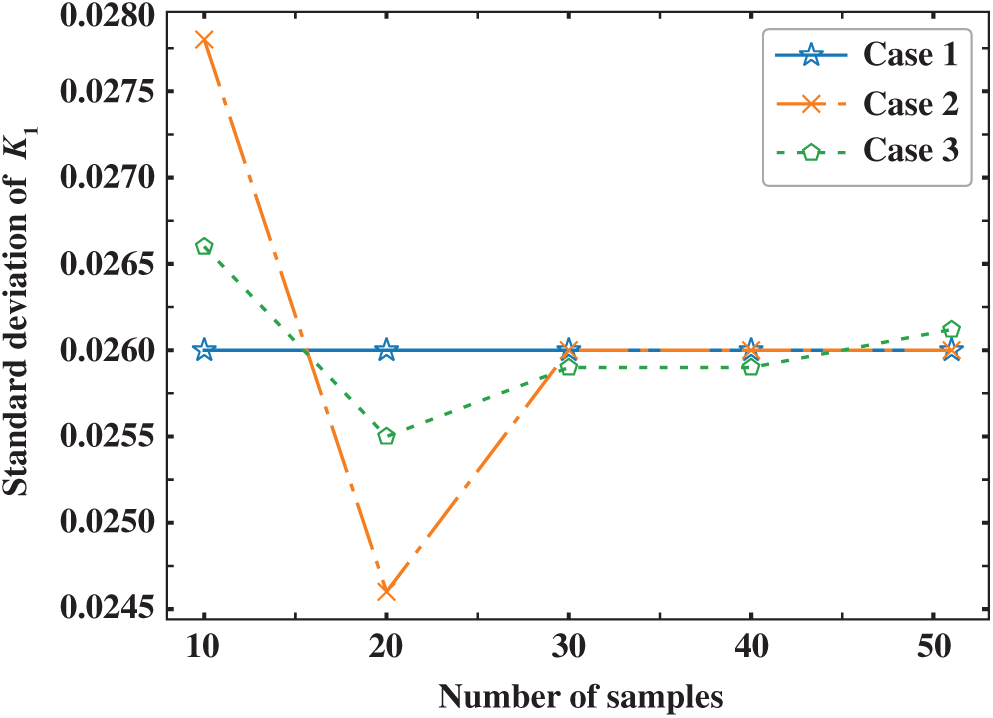
Figure 5: Standard deviation of K1
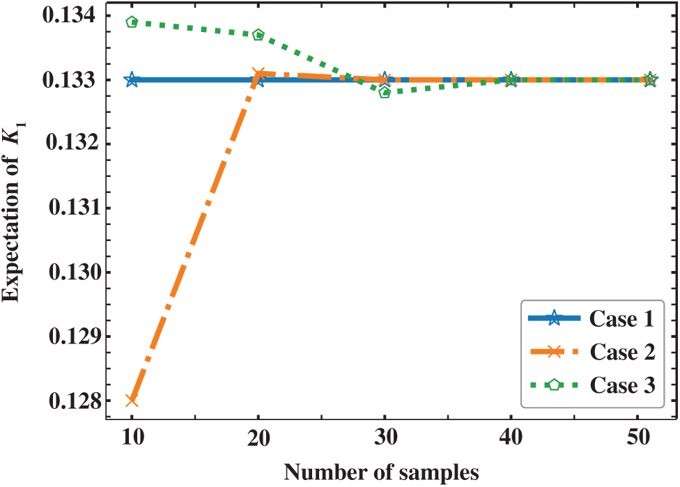
Figure 6: Expectation of K1
Now we fix the load ratio
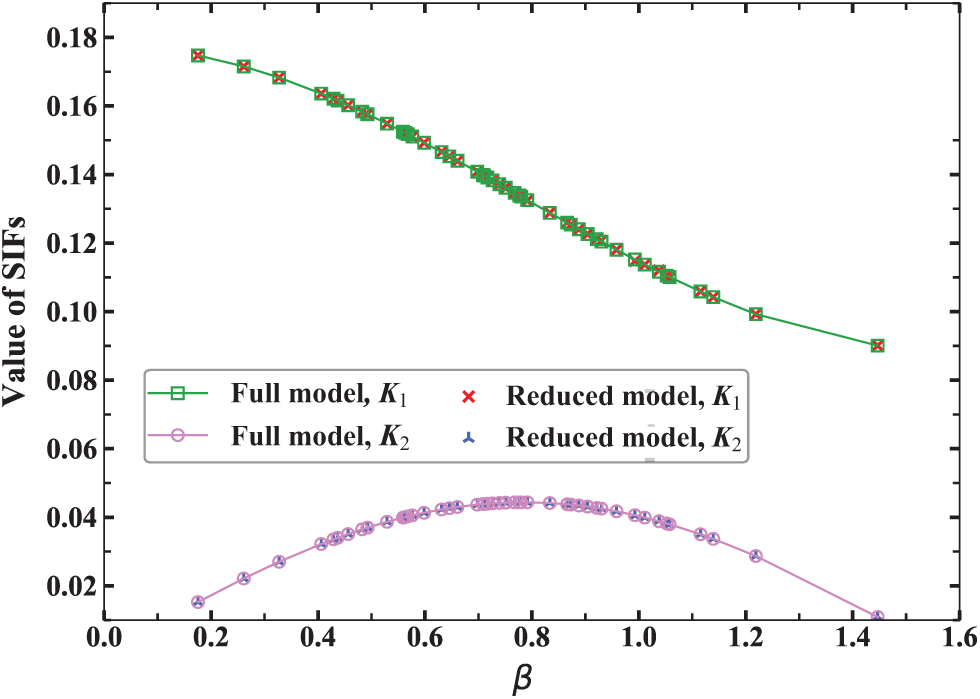
Figure 7: The value of SIFs obtained by using FOM and ROM
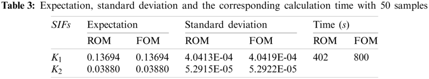
In this section, we further test the performance of this algorithm using an example of a plate with two rivet holes, as shown in Fig. 8. The Young’s modulus is E = 1000 and Poisson’s ratio
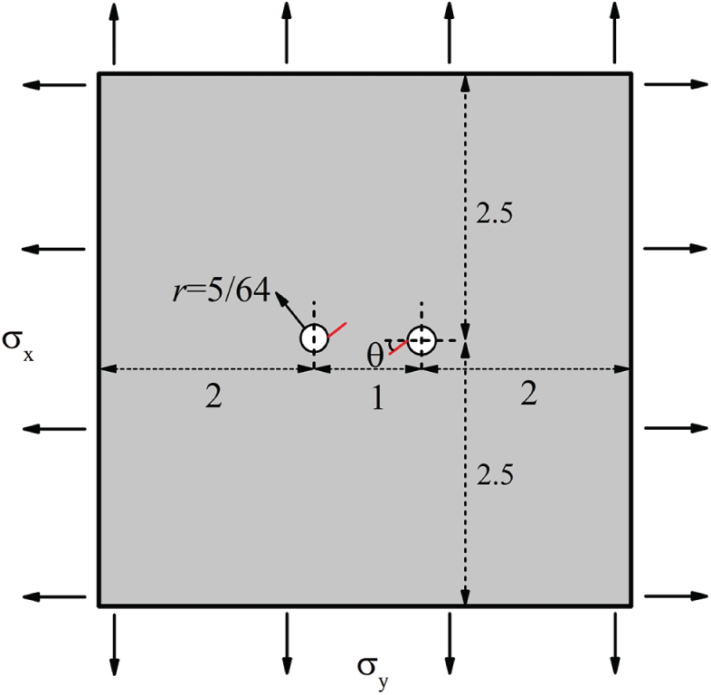
Figure 8: A plate with initial cracks emanating from the holes [58]
Suppose the radius
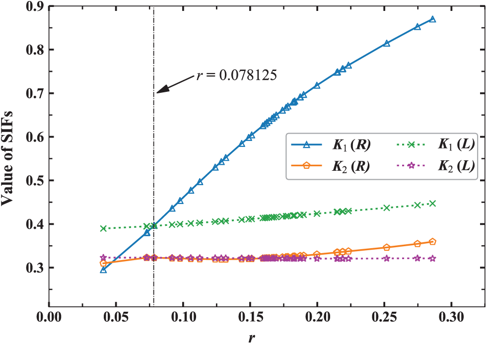
Figure 9: The value of SIFs for two crack surface with the input parameter
Now we consider the influence of material parameter on displacement of cracks. The elastic modulus
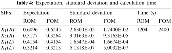
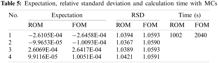
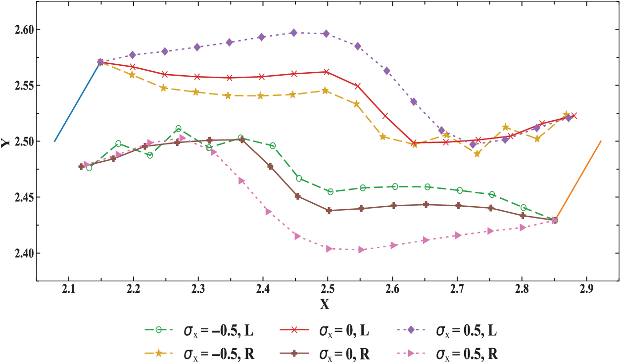
Figure 10: Crack propagation path under different loads
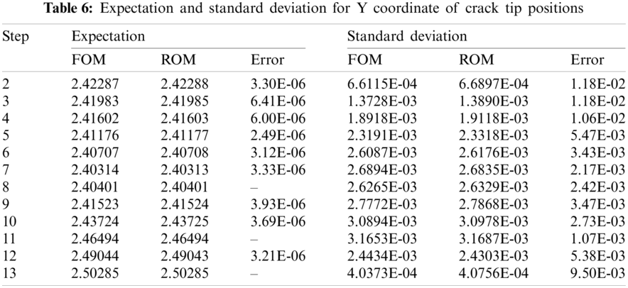
We also study how the crack propagation path is influenced by the input parameter of
The paper presents a novel framework for Monte Carlo simulation of multi-dimensional uncertainties of two-dimensional linear fracture mechanics. We use the NURBS to build the geometric model and discretize boundary integral equations. The IGABEM eliminates the repeatedly meshing procedure in uncertainty quantification, and retains the geometric exactness. The combination of POD and RBF accelerates the stochastic analysis and maintains good accuracy at low frequencies. In this work, the POD-RBF is used to approximate the structural response of a single random input variable. The method can also be extended to the problems with multidimensional random input variables, which will be investigated in the future. In addition, the present method will be applied to three dimensional problems and multi-physics coupling problems.
Funding Statement: The authors thank the financial support of National Natural Science Foundation of China (NSFC) under Grant (Nos. 51904202, 11902212, 11901578).
Conflicts of Interest: The authors declare that they have no conflicts of interest to report regarding the present study.
1. Stefanou, G. (2009). The stochastic finite element method: Past, present and future. Computer Methods in Applied Mechanics and Engineering, 198(9), 1031–1051. DOI 10.1016/j.cma.2008.11.007. [Google Scholar] [CrossRef]
2. Marcin, K. (2007). Generalized perturbation-based stochastic finite element method in elastostatics. Computers and Structures, 85(10), 586–594. DOI 10.1016/j.compstruc.2006.08.077. [Google Scholar] [CrossRef]
3. Ghanem, R., Spanos, P. (1991). Stochastic finite elements: A spectral approach. Berlin, Germany: Springer-Verlag. [Google Scholar]
4. Chen, N., Soares, C. (2008). Spectral stochastic finite element analysis for laminated composite plates. Computer Methods in Applied Mechanics and Engineering, 197(51–52), 4830–4839. DOI 10.1016/j.cma.2008.07.003. [Google Scholar] [CrossRef]
5. Hurtado, J., Barbat, A. (1998). Monte carlo techniques in computational stochastic mechanics. Archives of Computational Methods in Engineering, 5(1), 3–30. DOI 10.1007/BF02736747. [Google Scholar] [CrossRef]
6. Spanos, P., Zeldin, B. (1998). Monte carlo treatment of random fields: A broad perspective. Applied Mechanics Reviews, 51(3), 219–237. DOI 10.1115/1.3098999. [Google Scholar] [CrossRef]
7. Feng, Y., Li, C., Owen, D. (2010). A directed monte carlo solution of linear stochastic algebraic system of equations. Finite Elements in Analysis and Design, 46(6), 462–473. DOI 10.1016/j.finel.2010.01.004. [Google Scholar] [CrossRef]
8. Broomhead, D., Lowe, D. (1998). Radial basis functions, multi-variable functional interpolation and adaptive networks. Royal signals and radar establishment. The Annals of Statistics, 26(3), 801–849. [Google Scholar]
9. Buljak, V., Maier, G. (2011). Proper orthogonal decomposition and radial basis functions in material characterization based on instrumented indentation. Engineering Structures, 33(2), 492–501. DOI 10.1016/j.engstruct.2010.11.006. [Google Scholar] [CrossRef]
10. Buljak, V. (2012). Proper orthogonal decomposition and radial basis functions for fast simulations. Inverse analyses with model reduction, pp. 85–139. Berlin, Germany: Springer. [Google Scholar]
11. Rogers, C., Kassab, A., Divo, E., Ostrowski, Z., Bialecki, R. (2012). An inverse pod-RBF network approach to parameter estimation in mechanics. Inverse Problems in Science and Engineering, 20(5), 749–767. DOI 10.1080/17415977.2012.693080. [Google Scholar] [CrossRef]
12. Pinnau, R. (2008). Model reduction via proper orthogonal decomposition. Berlin Heidelberg: Springer. [Google Scholar]
13. Chinesta, F., Ladeveze, P., Cueto, E. (2011). A short review on model order reduction based on proper generalized decomposition. Archives of Computational Methods in Engineering, 18(4), 395–404. DOI 10.1007/s11831-011-9064-7. [Google Scholar] [CrossRef]
14. Kerfriden, P., Goury, O., Rabczuk, T., Bordas, S. (2013). A partitioned model order reduction approach to rationalise computational expenses in nonlinear fracture mechanics. Computer Methods in Applied Mechanics and Engineering, 256(5), 169–188. DOI 10.1016/j.cma.2012.12.004. [Google Scholar] [CrossRef]
15. Ding, C., Deokar, R., Cui, X., Li, G., Cai, Y. et al. (2019). Proper orthogonal decomposition and monte carlo based isogeometric stochastic method for material, geometric and force multi-dimensional uncertainties. Computational Mechanics, 63(3), 521–533. DOI 10.1007/s00466-018-1607-4. [Google Scholar] [CrossRef]
16. Li, S., Trevelyan, J., Wu, Z., Lian, H., Wang, D. et al. (2019). An adaptive SVD-Krylov reduced order model for surrogate based structural shape optimization through isogeometric boundary element method. Computer Methods in Applied Mechanics and Engineering, 349(1), 312– 338. DOI 10.1016/j.cma.2019.02.023. [Google Scholar] [CrossRef]
17. Hughes, T., Cottrell, J., Bazilevs, Y. (2005). Isogeometric analysis: CAD, finite elements, NURBS, exact geometry and mesh refinement. Computer Methods in Applied Mechanics and Engineering, 194(39–41), 4135–4195. DOI 10.1016/j.cma.2004.10.008. [Google Scholar] [CrossRef]
18. Bazilevs, Y., Michler, C., Calo, V., Hughes, T. (2010). Isogeometric variational multiscale modeling of wall-bounded turbulent flows with weakly enforced boundary conditions on unstretched meshes. Computer Methods in Applied Mechanics and Engineering, 199(13–16), 780–790. DOI 10.1016/j.cma.2008.11.020. [Google Scholar] [CrossRef]
19. Nguyen-Thanh, N., Kiendl, J., Nguyen-Xuan, H., Wüchner, R., Bletzinger, K. et al. (2011). Rotation free isogeometric thin shell analysis using PHT-splines. Computer Methods in Applied Mechanics and Engineering, 200(47–48), 3410–3424. DOI 10.1016/j.cma.2011.08.014. [Google Scholar] [CrossRef]
20. Wang, P., Xu, J., Deng, J., Chen, F. (2011). Adaptive isogeometric analysis using rational PHT-splines. Computer-Aided Design, 43(11), 1438–1448. DOI 10.1016/j.cad.2011.08.026. [Google Scholar] [CrossRef]
21. Cirak, F., Scott, M., Antonsson, E., Ortiz, M., Schröder, P. (2002). Integrated modeling, finite-element analysis, and engineering design for thin-shell structures using subdivision. Computer-Aided Design, 34(2), 137–148. DOI 10.1016/S0010-4485(01)00061-6. [Google Scholar] [CrossRef]
22. Banerjee, P., Cathie, D. (1980). A direct formulation and numerical implementation of the boundary element method for two-dimensional problems of elasto-plasticity. International Journal of Mechanical Sciences, 22(4), 233–245. DOI 10.1016/0020-7403(80)90038-7. [Google Scholar] [CrossRef]
23. Cruse, T. (1996). Bie fracture mechanics analysis: 25 years of developments. Computational Mechanics, 18(1), 1–11. DOI 10.1007/BF00384172. [Google Scholar] [CrossRef]
24. Seybert, A., Soenarko, B., Rizzo, F., Shippy, D. (1985). An advanced computational method for radiation and scattering of acoustic waves in three dimensions. The Journal of the Acoustical Society of America, 77(2), 362–368. DOI 10.1121/1.391908. [Google Scholar] [CrossRef]
25. Liu, Y. (2015). Analysis of shell-like structures by the boundary element method based on 3-D elasticity: Formulation and verification. International Journal for Numerical Methods in Engineering, 41(3), 541–558. DOI 10.1002/(SICI)1097-0207(19980215)41:3¡541::AID-NME298¿3.0.CO;2-K. [Google Scholar] [CrossRef]
26. Gu, Y., Gao, H., Chen, W., Zhang, C. (2016). A general algorithm for evaluating nearly singular integrals in anisotropic three-dimensional boundary element analysis. Computer Methods in Applied Mechanics and Engineering, 308(15), 483–498. DOI 10.1016/j.cma.2016.05.032. [Google Scholar] [CrossRef]
27. Gu, J., Zhang, J., Li, G. (2012). Isogeometric analysis in BIE for 3-D potential problem. Engineering Analysis with Boundary Elements, 36(5), 858–865. DOI 10.1016/j.enganabound.2011.09.018. [Google Scholar] [CrossRef]
28. Campos, L., Albuquerque, E., Wrobel, L. (2017). An ACA accelerated isogeometric boundary element analysis of potential problems with non-uniform boundary conditions. Engineering Analysis with Boundary Elements, 80(39), 108–115. DOI 10.1016/j.enganabound.2017.04.004. [Google Scholar] [CrossRef]
29. Gong, Y., Dong, C., Qin, X. (2017). An isogeometric boundary element method for three dimensional potential problems. Journal of Computational and Applied Mathematics, 313, 454–468. DOI 10.1016/j.cam.2016.10.003. [Google Scholar] [CrossRef]
30. Gong, Y., Dong, C., Bai, Y. (2017). Evaluation of nearly singular integrals in isogeometric boundary element method. Engineering Analysis with Boundary Elements, 75(3), 21–35. DOI 10.1016/j.enganabound.2016.11.005. [Google Scholar] [CrossRef]
31. Takahashi, T., Matsumoto, T. (2012). An application of fast multipole method to isogeometric boundary element method for laplace equation in two dimensions. Engineering Analysis with Boundary Elements, 36(12), 1766–1775. DOI 10.1016/j.enganabound.2012.06.004. [Google Scholar] [CrossRef]
32. Simpson, R., Bordas, S., Lian, H., Trevelyan, J. (2013). An isogeometric boundary element method for elastostatic analysis: 2D implementation aspects. Computers & Structures, 118(3), 2–12. DOI 10.1016/j.compstruc.2012.12.021. [Google Scholar] [CrossRef]
33. Scott, M., Simpson, R., Evans, J., Lipton, S., Bordas, S. et al. (2013). Isogeometric boundary element analysis using unstructured T-splines. Computer Methods in Applied Mechanics and Engineering, 254(21–26), 197–221. DOI 10.1016/j.cma.2012.11.001. [Google Scholar] [CrossRef]
34. Gu, J., Zhang, J., Chen, L., Cai, Z. (2015). An isogeometric BEM using PB-spline for 3-D linear elasticity problem. Engineering Analysis with Boundary Elements, 56(11), 154–161. DOI 10.1016/j.enganabound.2015.02.013. [Google Scholar] [CrossRef]
35. Han, Z., Cheng, C., Hu, Z., Niu, Z. (2018). The semi-analytical evaluation for nearly singular integrals in isogeometric elasticity boundary element method. Engineering Analysis with Boundary Elements, 95(39), 286–296. DOI 10.1016/j.enganabound.2018.07.016. [Google Scholar] [CrossRef]
36. Wang, Y., Benson, D. (2015). Multi-patch nonsingular isogeometric boundary element analysis in 3D. Computer Methods in Applied Mechanics and Engineering, 293(41), 71–91. DOI 10.1016/j.cma.2015.03.016. [Google Scholar] [CrossRef]
37. Simpson, R., Scott, M., Taus, M., Thomas, D., Lian, H. (2014). Acoustic isogeometric boundary element analysis. Computer Methods in Applied Mechanics and Engineering, 269(139), 265–290. DOI 10.1016/j.cma.2013.10.026. [Google Scholar] [CrossRef]
38. Keuchel, S., Hagelstein, N., Zaleski, O., von Estorff, O. (2017). Evaluation of hypersingular and nearly singular integrals in the isogeometric boundary element method for acoustics. Computer Methods in Applied Mechanics and Engineering, 325(10), 488–504. DOI 10.1016/j.cma.2017.07.025. [Google Scholar] [CrossRef]
39. Chen, L., Marburg, S., Zhao, W., Liu, C., Chen, H. (2019). Implementation of isogeometric fast multipole boundary element methods for 2D half-space acoustic scattering problems with absorbing boundary condition. Journal of Theoretical and Computational Acoustics, 27(2), 1850024. DOI 10.1142/S259172851850024X. [Google Scholar] [CrossRef]
40. Chen, L., Lian, H., Liu, Z., Chen, H., Atroshchenko, E. et al. (2019). Structural shape optimization of three dimensional acoustic problems with isogeometric boundary element methods. Computer Methods in Applied Mechanics and Engineering, 355(2), 926–951. DOI 10.1016/j.cma.2019.06.012. [Google Scholar] [CrossRef]
41. Chen, L., Liu, C., Zhao, W., Liu, L. (2018). An isogeometric approach of two dimensional acoustic design sensitivity analysis and topology optimization analysis for absorbing material distribution. Computer Methods in Applied Mechanics and Engineering, 336(39), 507–532. DOI 10.1016/j.cma.2018.03.025. [Google Scholar] [CrossRef]
42. Liu, C., Chen, L., Zhao, W., Chen, H. (2017). Shape optimization of sound barrier using an isogeometric fast multipole boundary element method in two dimensions. Engineering Analysis with Boundary Elements, 85, 142–157. DOI 10.1016/j.enganabound.2017.09.009. [Google Scholar] [CrossRef]
43. Chen, L., Zhang, Y., Lian, H., Atroshchenko, E., Bordas, S. (2020). Seamless integration of computer-aided geometric modeling and acoustic simulation: Isogeometric boundary element methods based on Catmull–Clark subdivision surfaces. Advances in Engineering Software, 149(2), 102879. DOI 10.1016/j.advengsoft.2020.102879. [Google Scholar] [CrossRef]
44. Chen, L., Lu, C., Zhao, W., Chen, H., Zheng, C. J. (2020). Subdivision surfaces-boundary element accelerated by fast multipole for the structural acoustic problem. Journal of Theoretical and Computational Acoustics, 28(2), 2050011. DOI 10.1142/S2591728520500115. [Google Scholar] [CrossRef]
45. Simpson, R., Liu, Z., Vazquez, R., Evans, J. (2018). An isogeometric boundary element method for electromagnetic scattering with compatible B-spline discretizations. Journal of Computational Physics, 362(39), 264–289. DOI 10.1016/j.jcp.2018.01.025. [Google Scholar] [CrossRef]
46. Li, K., Qian, X. (2011). Isogeometric analysis and shape optimization via boundary integral. Computer-Aided Design, 43(11), 1427–1437. DOI 10.1016/j.cad.2011.08.031. [Google Scholar] [CrossRef]
47. Lian, H., Kerfriden, P., Bordas, S. (2016). Implementation of regularized isogeometric boundary element methods for gradient-based shape optimization in two-dimensional linear elasticity. International Journal for Numerical Methods in Engineering, 106(12), 972–1017. DOI 10.1002/nme.5149. [Google Scholar] [CrossRef]
48. Lian, H., Kerfriden, P., Bordas, S. (2017). Shape optimization directly from CAD: An isogeometric boundary element approach using T-splines. Computer Methods in Applied Mechanics and Engineering, 317(4), 1–41. DOI 10.1016/j.cma.2016.11.012. [Google Scholar] [CrossRef]
49. Chen, L., Lu, C., Lian, H., Liu, Z., Zhao, W. et al. (2020). Acoustic topology optimization of sound absorbing materials directly from subdivision surfaces with isogeometric boundary element methods. Computer Methods in Applied Mechanics and Engineering, 362(3–5), 112806. DOI 10.1016/j.cma.2019.112806. [Google Scholar] [CrossRef]
50. Peng, X., Atroshchenko, E., Kerfriden, P., Bordas, S. (2017). Linear elastic fracture simulation directly from CAD: 2D nurbs-based implementation and role of tip enrichment. International Journal of Fracture, 204(1), 55–78. DOI 10.1007/s10704-016-0153-3. [Google Scholar] [CrossRef]
51. Peng, X., Atroshchenko, E., Kerfriden, P., Bordas, S. (2017). Isogeometric boundary element methods for three dimensional static fracture and fatigue crack growth. Computer Methods in Applied Mechanics and Engineering, 316(23–24), 151–185. DOI 10.1016/j.cma.2016.05.038. [Google Scholar] [CrossRef]
52. Doucet, A., Freitas, N., Gordon, N. (2001). Sequential monte carlo methods in practice. New York, NY: Springer. [Google Scholar]
53. Hong, H., Chen, J. (1988). Derivations of integral equations of elasticity. Journal of Engineering Mechanics, 114(6), 1028–1044. DOI 10.1061/(ASCE)0733-9399(1988)114:6(1028). [Google Scholar] [CrossRef]
54. Yau, J., Wang, S., Corten, H. (1980). A mixed-mode crack analysis of isotropic solids using conservation laws of elasticity. Journal of Applied Mechanics, 47(2), 335–341. DOI 10.1115/1.3153665. [Google Scholar] [CrossRef]
55. Erdogan, F., Sih, G. (1963). On the crack extension in plates under plane loading and transverse shear. Journal of Basic Engineering, 85(4), 519–525. DOI 10.1115/1.3656897. [Google Scholar] [CrossRef]
56. Smith, D., Ayatollahi, M., Pavier, M. (2001). The role of T-stress in brittle fracture for linear elastic materials under mixed-mode loading. Fatigue & Fracture of Engineering Materials & Structures, 24(2), 137–150. DOI 10.1046/j.1460-2695.2001.00377.x. [Google Scholar] [CrossRef]
57. Wang, D., Wu, Z., Fei, Y., Zhang, W. (2014). Structural design employing a sequential approximation optimization approach. Computers and Structures, 134(4598), 75–87. DOI 10.1016/j.compstruc.2013.12.004. [Google Scholar] [CrossRef]
58. Moës, N., Dolbow, J., Belytschko, T. (1999). A finite element method for crack growth without remeshing. International Journal for Numerical Methods in Engineering, 46(1), 131–150. DOI 10.1002/(SICI)1097-0207(19990910)46:1¡131::AID-NME726¿3.0.CO;2-J. [Google Scholar] [CrossRef]
Appendix A: Fundamental Solution
The fundamental solutions of displacement integral equation
The fundamental solutions of traction integral equation D*ijk and S*ijk are
Appendix B: Evaluation of Stress Intensity Factors
The M integral based on the J integral is an effective method to extract SIFs. The Jk integral is defined as follows:
where Pkj is the Eshelby tensor, strain energy density
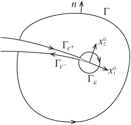
Figure A.1: J integral
Now, consider two independent equilibrium states of an elastically deformable object, the actual state (superscript ‘1’) and the auxiliary state (superscript ‘2’). Superimpose these two equilibrium states into one equilibrium state. It is assumed that the crack surface is flat in a sufficiently small radius of the contour circle. The conservation law can be reduced to the path-independent J integral along an arbitrary path
Rearranging Eq. (B.2) into the following formulas:
where
with W(1, 2) being the mutual potential energy density of the elastic body.
The J integral under two states can be expressed as a function associated with K, as follows:
where
Upon substitution of Eq. (B.3) into (B.5), we can obtain new expression of the M integral, as follows:
The M integral shown in Eqs. (B.4) and (B.6) only involves interaction terms, which can be directly used to solve the mixed mode crack problem of linear elastic solids.
After SIFs are calculated, the direction of crack propagation can be determined by the maximum hoop stress criterion, the discriminant equation is as follows:
where
 | This work is licensed under a Creative Commons Attribution 4.0 International License, which permits unrestricted use, distribution, and reproduction in any medium, provided the original work is properly cited. |