| Computer Modeling in Engineering & Sciences |
DOI: 10.32604/cmes.2021.016794
ARTICLE
Subdivision Surface-Based Isogeometric Boundary Element Method for Steady Heat Conduction Problems with Variable Coefficient
1School of Architectural Engineering, Huanghuai University, Zhumadian, 463003, China
2College of Intelligent Construction, Wuchang University of Technology, Wuhan, 430223, China
3College of Civil Engineering and Architecture, China Three Gorges University, Yichang, 443000, China
4CAS Key Laboratory of Mechanical Behavior and Design of Materials, Department of Modern Mechanics, University of Science and Technology of China, Hefei, 230026, China
*Corresponding Author: Yanming Xu. Email: cat2@mail.ustc.edu.cn
Received: 26 March 2021; Accepted: 08 May 2021
Abstract: The present work couples isogeometric analysis (IGA) and boundary element methods (BEM) for three dimensional steady heat conduction problems with variable coefficients. The Computer-Aided Design (CAD) geometries are built by subdivision surfaces, and meantime the basis functions of subdivision surfaces are employed to discretize the boundary integral equations for heat conduction analysis. Moreover, the radial integration method is adopted to transform the additional domain integrals caused by variable coefficients to the boundary integrals. Several numerical examples are provided to demonstrate the correctness and advantages of the proposed algorithm in the integration of CAD and numerical analysis.
Keywords: Subdivision surface; isogeometric boundary element method; heat conduction; radial integration
Since the pioneering work of Hughes et al. [1], isogeometric analysis (IGA) has attracted extensive attention from academia and industry. Different from the traditional numerical methods based on Lagrange polynomials, IGA employs the same basis functions used for geometric modeling in Computer-Aided Design (CAD), such as Non-Uniform Rational B-splines (NURBS) to discretize the unknown physical fields in Partial Differential Equations. Due to the capability of integrating CAD and numerical analysis, IGA is able to eliminate cumbersome meshing procedures, guaranteeing geometric exactness, and offering high-order continuous approximation and flexible refinement schemes [2–6]. In order to ease the implementation of IGA, Bézier extraction operation [7] is introduced, which also accelerates the evaluation of basis functions significantly.
The concept of IGA was first proposed in the context of finite element methods (FEM). Its application in engineering practice for complex geometries is limited due to the volume parameterization of FEM conflicts with the boundary representation of CAD. On the contrary, the boundary element method (BEM) only needs boundary parameterization and thus is naturally compatible with CAD model [8–12]. The isogeometric boundary element method (IGABEM) has been successfully applied to many fields, including linear elasticity [13–16], potential problems [17–20], fracture mechanics [21–25], electromagnetics [26], acoustics [27–32], structural optimization [33–37].
Heat conduction is of paramount importance in engineering. IGABEM based on NURBS was applied to 3D steady thermal conduction problems for a medium with non-homogenous inclusions [38,39] and transient heat conduction problems with heat sources [40–46]. In the present paper, we adopts IGABEM based on subdivision surfaces for simulating steady heat conduction problems with variable coefficients. The subdivision surface method is a CAD technology which was first proposed by Catmull et al. [47]. Compared to NURBS or other CAD modeling techniques, a salient feature of the subdivision surface method is that it is capable of constructing water-tight geometries and address extraordinary (or irregular) points [48]. Cirak et al. [49] combined the subdivision surface method with the FEM to simulate the deformation of thin shell structures. Green et al. [50] put forward a multi-level method based on subdivision surfaces for accelerating the analysis of large-scale thin shell problems. The multi-resolution subdivision surfaces were also used for structural shape optimization in electromagnetic fields [51]. For heat conduction problems with variable thermal conductivity coefficients, an addition domain integral term appears in the boundary integral equations. To solve this problem, the radial basis function method (RBF) was proposed to transform the domain integral to the boundary integral in conventional BEM [52,53]. Such RBF method is also incorporated to the present work with IGABEM.
The remainder of the paper is organized as follows. The Catmull–Clark subdivision surface method is introduced in Section 2. The IGABEM with subdivision surfaces is used for solution of heat conduction with variable coefficient in Section 3. Then, several numerical examples are discussed in Section 4, followed by the conclusion in Section 5.
2 Subdivision Surface Method Based on Catmull–Clark
Subdivision surface is defined as the limit of an infinite refinement or subdivision process. Each new subdivision step produces a new mesh with more polygonal elements and smoother geometries. By repeatedly refining the initial polygon mesh, a series of meshes that approach the final subdivision surface is generated. The subdivision surface inherits the reconfigurability of spline curve, so that all control meshes generated in subdivision process can accurately represent the same spline surface. An important technical advance in subdivision surfaces is to generate limiting surfaces by constructing an elementwise mapping from the subdivided meshes. In this way, the subdivided meshes play the same role as control grids of NURBS in geometry modeling, and the limiting surface resembles the physical surface in NURBS.
In this work we consider the quadrilateral subdivision surfaces proposed by Catmull–Clark. The Catmull–Clark subdivision scheme is an extension of bicubic uniform B-splines. Catmull–Clark subdivision algorithm subdivides each quadrilateral element into four sub-quadrilateral elements (1–4 splitting) as shown in Fig. 1. After continuous subdivision operation, the ultimate surface is obtained.
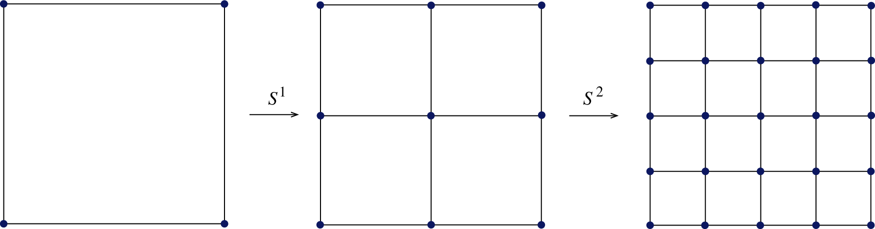
Figure 1: Catmull–Clark subdivision process
Let us set the original mesh subdivision level as k, and then subdivide it into k + 1 level. The vertices on the k level mesh are weighted on their patches to obtain new vertices on the k + 1 level mesh, which are represented by the symbol “V”. Four new vertices are inserted at the midpoints of four edges at every element for the k level mesh, which are represented by the symbol “E”. In addition, a new vertex is inserted at the center of every element for the k level mesh, which is represented by the symbol “F”. An edge passing through a “V” vertex on the k level mesh is called this vertex’s adjacent edge. The number of adjacent edges to a vertex is called a valence nv of this vertex. If nv = 4, the vertex is called a regular vertex as shown in Fig. 2 (blue point), otherwise it is called an irregular vertex as shown in Fig. 2 (red point), and the symbol “u” denotes the valence nv of Point 1.
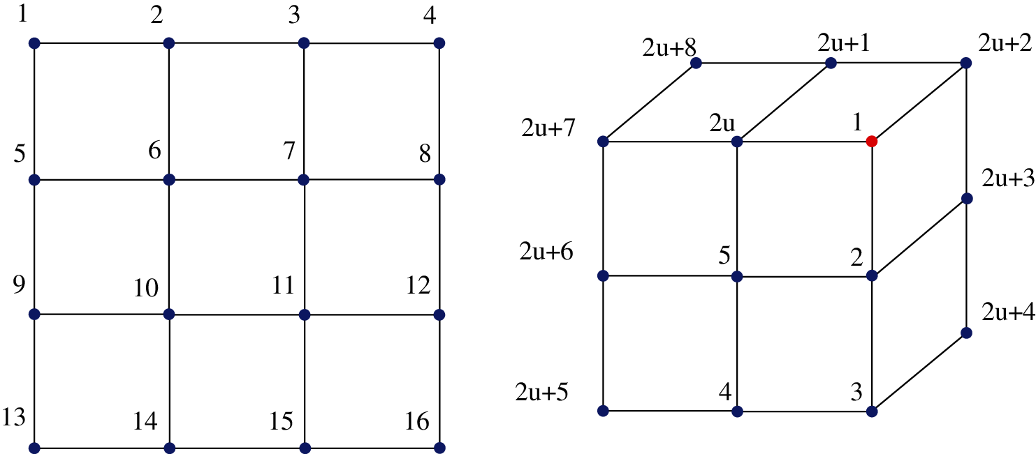
Figure 2: The regular and irregular points of Catmull–Clark subdivision surface
A quadrilateral mesh can be divided into four sub-elements by inserting a new point in the middle of each edge and inside the element, which are called “E” and “F”, respectively. In addition, the position of original points called “V” is moved to construct smooth surface flexibly.
The coordinates of these vertices “V”, “E” and “F” on the k + 1 level mesh generated after one subdivision are obtained from that on the k level mesh by interpolation operation, as follows:
where
The idea of limit subdivision is used to subdivide the irregular elements locally and repeatedly through the following steps: (1) introducing subdivision matrices to establish the relationship between the hierarchical sub units and the parent units, (2) obtaining the eigenvector and eigenvalue of the matrix by Fourier transformation of the subdivision matrix, (3) storing the information of the hierarchical regular sub units by using the subdivision matrix, the picking matrix and the regular unit, and (4) building the base function of the original irregular parent unit 3. After constructing the basis function of the irregular element, the surface model corresponding to the whole mesh can be constructed by the fitting operation, and the model has C2 continuity at the regular point and C1 continuity at the irregular point.
In each regular quadrilateral there are sixteen quartic non-zero basis functions associated with its and neighbouring quadrilateral vertices, as shown in Fig. 3. Hence, the surface coordinates Xe within the quadrilateral e can be determined through
where Xi denotes the coordinate of the i-th adjacent vertex, the parameter field satisfies
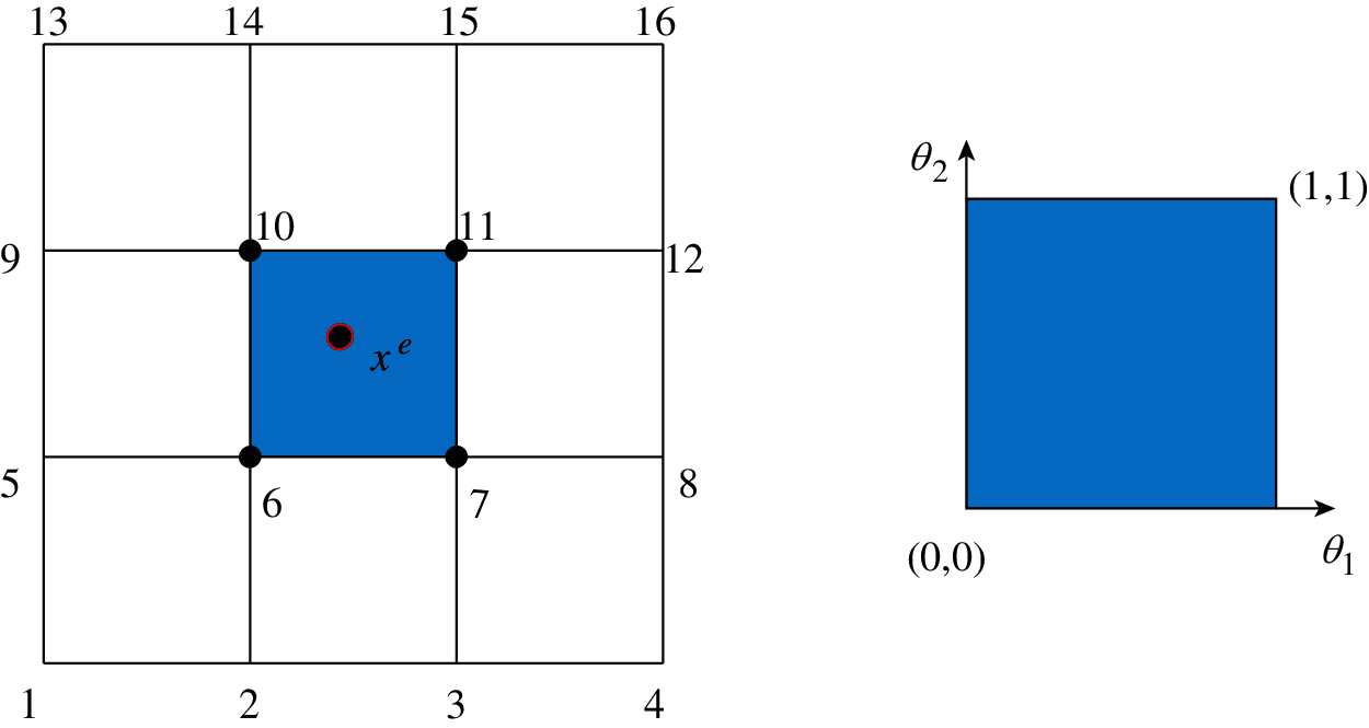
Figure 3: The Cartesian coordinates of the fitting element and the parameter field
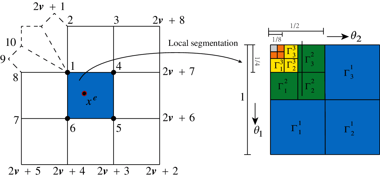
Figure 4: Local segmentation
As shown in Fig. 4, the local subdivision process of irregular cells can be used to devise an algorithm for obtaining subdivision basis functions Bir for quadrilateral patches that contain irregular vertices, as follows:
where
3 IGABEM for Heat Conduction with Subdivision Surface
3.1 Governing Equation of Heat Conduction
The governing differential equation of steady-state heat conduction in isotropic media with variable coefficient and internal heat source is expressed as follows:
where k(x) is the thermal conductivity, Q(x) is the heat source value at the point x, the boundary condition is expressed as follows:
where ΓT represents a constant temperature boundary, Γq represents a constant temperature flux boundary, and n(x) is the outer normal vector at point x.
By introducing weight function
For the first term, by using the integral by parts method and Gauss divergence theorem, we can get the following formula:
The fundamental solution
and
By substituting Eq. (10) into Eq. (8), we can obtain the following integral equation containing the source term:
where the coefficient c(x) = 1 when the source point x is located in the domain, and c(x) = 0.5 when the source point is on the boundary of structure. The integrals in the above formula are expressed as follows:
where
By observing Eq. (11), we notice that the second and third terms are boundary integrals, but the last two terms are domain integrals. Although direct domain discretization methods can be used, the advantage of dimensionality reduction of BEM cannot be retained. Hence, in this work, the source term is not considered, and the RBF method is used to transform the domain integral caused by thermal conductivity into the boundary integral.
3.2 Transformation of Domain Integral Caused by Thermal Conductivity
The second domain integral in Eq. (11) contains the unknown variable
where
where fi(r) is the radial basis function at the i-th collocation point with
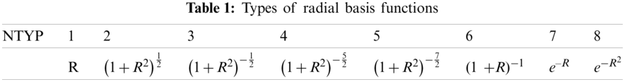
The commonly used radial basis functions are shown in Tab. 1. In this work, the third one is used for the solution of RBF.
How to determine the coefficients β and γ is particularly important. It is difficult to obtain these coefficients directly. However, through a series of transformation operations, we can get the implicit expression of these coefficients. When the point
where
and
where fij = fj (r) with r = |xi − xj|, and
It is worth noting that the matrix f is reversible when the collocation points are not repeated. Thus, the coefficient vector v can be expressed as
Upon substitution of Eq. (21) into Eq. (15), we arrive at
in which
By substituting Eq. (22) into the last term of Eq. (12) and using the radial integration method, the following boundary integral formula can be derived
where
We can find that the domain integral in Eq. (24) is successfully transformed into the boundary integral.
3.3 Discretization of IGABEM with Subdivision Surface
The boundary of domain is defined through the union of discretization elements, as follows:
In this work, the set of discretization elements
where the coefficients
where H* and G* are coefficient matrix of IGABEM with subdivision surface. V is the coefficient matrix obtained by Eq. (24), and yb is a known column vector formed by domain integral caused by heat source.
By substituting boundary conditions into Eq. (28), a system of linear algebraic equations can be obtained
The collocation approach is used to generate the linear system of equations of BEM. In this work, the collocation points are chosen as a series of points on the physical surface mapped from the nodes of the control mesh, or see [54] for detailed content. It should be noticed that when the heat flux q on boundary is known, the unknown variables x is the normalized temperature. By using the first term of Eq. (14), we can obtain the solution of real temperature.
4.1 A Cube with Cylindrical Hole
In this section, we consider a cube with cylindrical hole. Catmull–Clark subdivision surface scheme is used to construct a smooth model. The initial model is shown in Fig. 5a. The size of the cube is 0.5 m × 0.5 m × 0.5 m, and the radius of the cylinder in the middle of the cube is r = 0.125 m. Fig. 5b shows the model after subdivision once and Fig. 5c shows the model after subdivision twice. It is worth noting that although the control meshes at different subdivision levels are different, the surfaces obtained by fitting are the same and consistent with the limit subdivision mesh model. The temperature of the fluid in the cylinder is Tf = 293 K, and the convective heat transfer coefficient h = 1000 W/(m2· K) between the fluid and structure. The right surface of the structure with the maximum coordinate value in positive y-axis is subjected to constant heat flux q = 50000 W/m2. The other five surfaces are adiabatic. Material density ρ = 7800 kg/m3, specific heat capacity cp = 460 J/(kg · K), and thermal conductivity k = 500 W/(m · K).
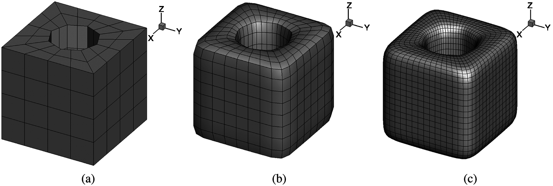
Figure 5: The cube model constructed by Catmull–Clark subdivision surface method. (a) Initial mesh (b) subdivision once (c) subdivision twice
Since there is no analytical solution to the problem, we compare the results of this algorithm proposed in this work with that of Fluent. In Fig. 6a, the coordinates of the computing points is (0.25, y, 0), and y ∈ [−0.25, 0.25]. The symbol “CC-IGABEM” denotes the numerical solution obtained from IGABEM with Catmull–Clark subdivision surfaces. In Fig. 6b, the computing points with z = 0.25 are located on the circumference of the circular hole, where θ denotes the angle between the vertical line from the computing point to the axis of the cylinder inside the structure and the x-axis. It can be seen that the results of the developed algorithm are consistent with those of fluent, which verifies the correctness of the algorithm.
We consider a problem with variable heat conduction coefficients. The thermal conductivity of the material is not a constant value, but satisfies k = (400 + 200r) W/(m · K). The distribution of temperature on structural surface for constant coefficient and variable coefficient is shown in Figs. 7a and 7b, respectively. It can be seen that the temperature field is symmetric along xoy and zoy planes, respectively. The right surface in contact with the constant heat flux has a higher temperature value than the left surface.
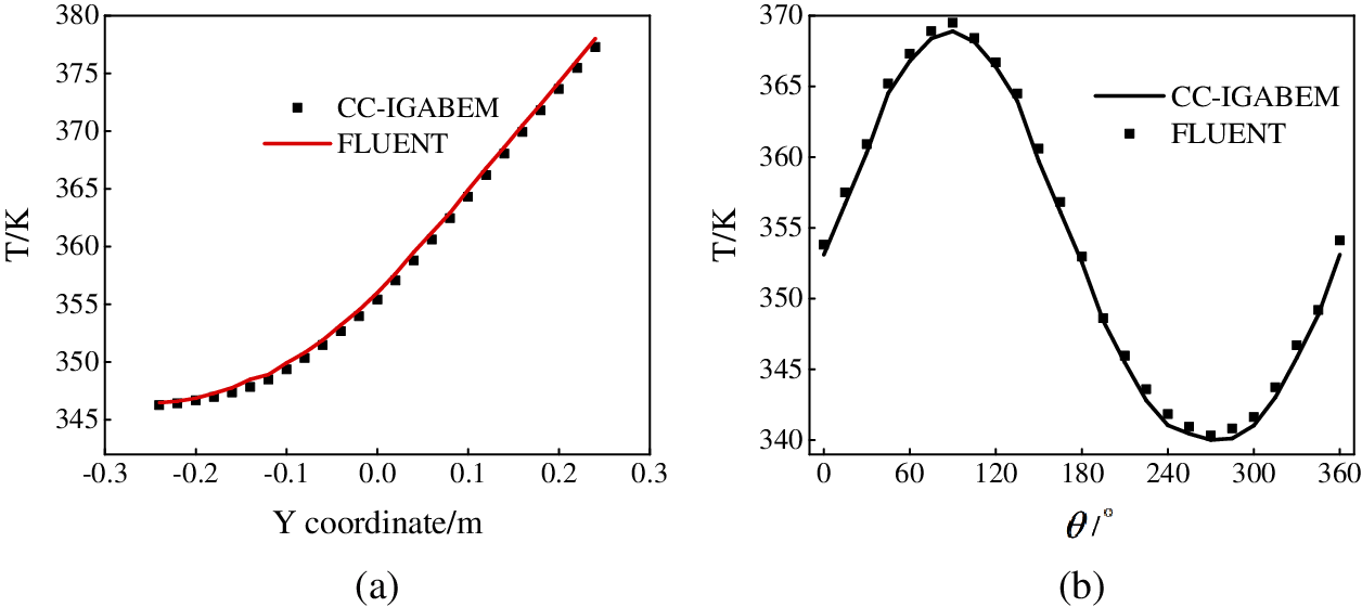
Figure 6: The temperature at several computing points obtained by using fluent and IGABEM with subdivision surface. (a) results at the points (0.25, y, 0) (b) results at the points z = 0.25
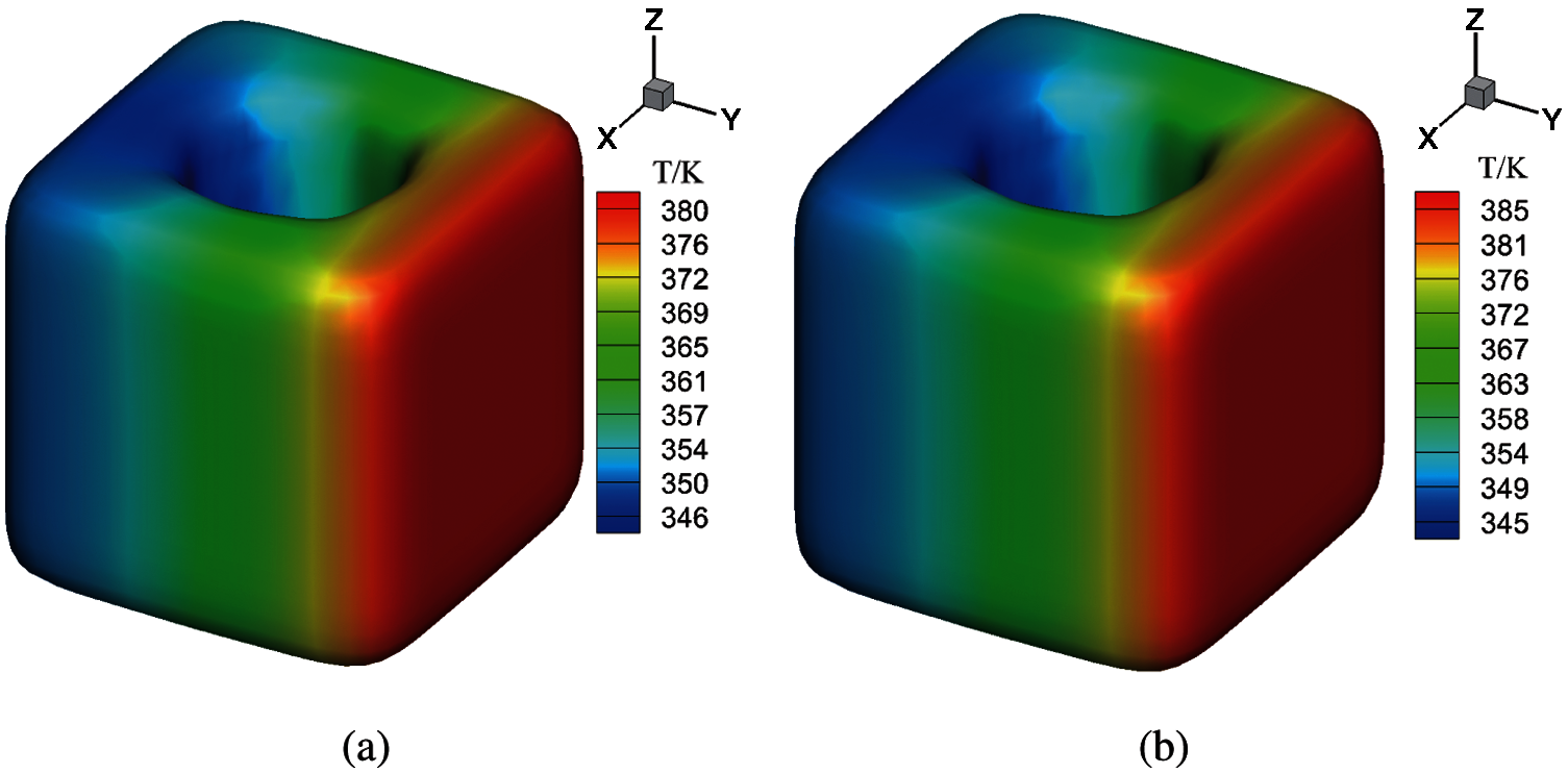
Figure 7: Distribution of temperature on structural surface. (a) Temperature distribution for constant thermal conductivity (b) temperature distribution for variable thermal conductivity
The value of the temperature at the computing points in Fig. 6a for homogeneous and heterogeneous materials are plotted in Fig. 8. For these two different conditions, there is a small difference between the calculation results, which shows that the variable heat conductivity has an impact on the calculation results, and also demonstrates the ability of the algorithm in this paper for variable coefficient problems.
Consider a dumbbell model shown in Fig. 9a. The top and bottom of the dumbbell is a hexahedron with a side length 0.08 m and height 0.08 m. The middle part of the dumbbell structure is a cylinder with a radius 0.04 m and height 0.16 m.
The top surface is subjected to constant heat flux q = 50000 W/m2. The bottom of the structure contacts a heat source with Tf = 293 K, and the convective heat transfer coefficient h = 1000 W/(m2 · K). The other surfaces are adiabatic. Herein, material density is ρ = 7800 kg/m3, heat capacity ratio is cp = 460 J/(kg · K), the thermal conductivity is k = 500 W/(m · K).

Figure 8: Distribution of temperature on structural surface
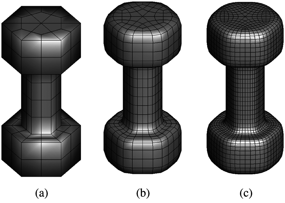
Figure 9: Initial cube and subdivision model of columnar body. (a) Initial mesh (b) subdivision once (c) subdivision twice
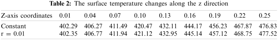
As shown in Fig. 9, the initial mesh in Fig. 9a is subdivided into denser grids, such as primary subdivision mesh in Fig. 9b and secondary subdivision mesh in Fig. 9c. Fig. 10 shows the distribution of temperature on the structural surface with constant thermal conductivity and variable thermal conductivity, respectively. The thermal conductivity of the material in Fig. 10b satisfies k = (400 + 200r) W/(m · K). The variable r denotes the distance from the point to the z-axis, which is the axis of symmetry in vertical direction. The temperature distribution decreases gradually along the z-axis. Although the temperature profiles corresponding to different thermal conductivities are very similar, the temperature values represented by the profiles show differences, as listed in Tab. 2.
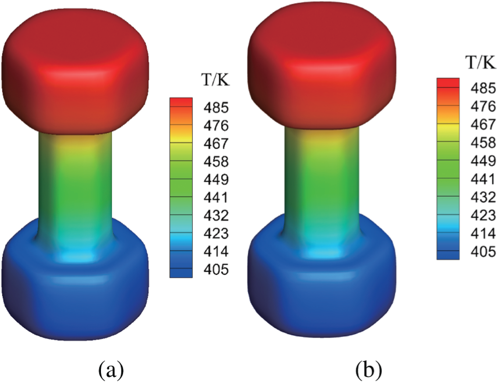
Figure 10: Temperature field with the change of thermal conductivity of columnar body. (a) Temperature distribution for constant thermal conductivity (b) temperature distribution for variable thermal conductivity
In this work, we present a novel framework for solving three-dimensional steady-state heat conduction problems with IGABEM. The Catmull–Clark subdivision surface method is used to construct a smooth geometric model and discretizing boundary integral equations. The radial integration method is incorporated to transform the domain integral caused by variable coefficient into the boundary integral. The numerical simulation can be conducted directly from CAD model without needing a meshing procedure. The numerical results validate the accuracy of the method and demonstrate its ability of integrating CAD and numerical analysis. In the future, we will extend the algorithm to transient heat conduction problems.
Funding Statement: The authors received no specific funding for this study.
Conflicts of Interest: The authors declare that they have no conflicts of interest to report regarding the present study.
1. Hughes, T. J. R., Cottrell, J. A., Bazilevs, Y. (2005). Isogeometric analysis: CAD, finite elements, nurbs, exact geometry and mesh refinement. Computer Methods in Applied Mechanics and Engineering, 194(39–41), 4135–4195. DOI 10.1016/j.cma.2004.10.008. [Google Scholar] [CrossRef]
2. Cottrell, J. A., Hughes, T. J. R., Reali, A. (2007). Studies of refinement and continuity in isogeometric structural analysis. Computer Methods in Applied Mechanics and Engineering, 196(41–44), 4160–4183. DOI 10.1016/j.cma.2007.04.007. [Google Scholar] [CrossRef]
3. Bazilevs, Y., Calo, V. M., Zhang, Y., Hughes, T. J. R. (2006). Isogeometric fluid-structure interaction analysis with applications to arterial blood flow. Computational Mechanics, 38(4–5), 310–322. DOI 10.1007/s00466-006-0084-3. [Google Scholar] [CrossRef]
4. Nagy, A. P., Abdalla, M. M., Guerdal, Z. (2006). Isogeometric sizing and shape optimisation of beam structures. Computer Methods in Applied Mechanics and Engineering, 199(17–20), 1216–1230. DOI 10.1016/j.cma.2009.12.010. [Google Scholar] [CrossRef]
5. Benson, D. J., Bazilevs, Y., Hsu, M. C., Hughes, T. J. R. (2010). Isogeometric shell analysis: The reissner-mindlin shell. Computer Methods in Applied Mechanics & Engineering, 199(5–8), 276–289. DOI 10.1016/j.cma.2009.05.011. [Google Scholar] [CrossRef]
6. Lorenzis, L. D., Temizer, I., Wriggers, P., Zavarise, G. (2011). A large deformation frictional contact formulation using nurbs-based isogeometric analysis. International Journal for Numerical Methods in Engineering, 87(13), 1278–1300. DOI 10.1002/nme.3159. [Google Scholar] [CrossRef]
7. Borden, M. J., Scott, M. A., Evans, J. A., Hughes, T. J. R. (2011). Isogeometric finite element data structures based on bézier extraction of nurbs. International Journal for Numerical Methods in Engineering, 87(1–5), 15–47. DOI 10.1002/nme.2968. [Google Scholar] [CrossRef]
8. Chen, L., Lu, C., Zhao, W., Chen, H., Zheng, C. (2020). Subdivision surfaces-boundary element accelerated by fast multipole for the structural acoustic problem. Journal of Theoretical and Computational Acoustics, 28(2), 2050011. DOI 10.1142/S2591728520500115. [Google Scholar] [CrossRef]
9. Zheng, C. J., Chen, H. B., Gao, H. F., Du, L. (2015). Is the burton-miller formulation really free of fictitious eigenfrequencies? Engineering Analysis with Boundary Elements, 59, 43–51. DOI 10.1016/j.enganabound.2015.04.014. [Google Scholar] [CrossRef]
10. Zheng, C. J., Zhao, W. C., Gao, H. F., Du, L., Zhang, Y. B. et al. (2021). Sensitivity analysis of acoustic eigenfrequencies by using a boundary element method. The Journal of the Acoustical Society of America, 149(3), 2027–2038. DOI 10.1121/10.0003622. [Google Scholar] [CrossRef]
11. Chen, L., Zheng, C., Chen, H., Marburg, S. (2016). Structural-acoustic sensitivity analysis of radiated sound power using a finite element/discontinuous fast multipole boundary element scheme. International Journal for Numerical Methods in Fluids, 82(12), 858–878. DOI 10.1002/fld.4244. [Google Scholar] [CrossRef]
12. Chen, L., Marburg, S., Chen, H., Zhang, H., Gao, H. (2017). An adjoint operator approach for sensitivity analysis of radiated sound power in fully coupled structural-acoustic systems. Journal of Computational Acoustics, 25(1), 1750003. DOI 10.1142/S0218396X17500035. [Google Scholar] [CrossRef]
13. Simpson, R. N., Bordas, S. P. A., Trevelyan, J., Rabczuk, T. (2012). A two-dimensional isogeometric boundary element method for elastostatic analysis. Computer Methods in Applied Mechanics and Engineering, 209–212, 87–100. DOI 10.1016/j.cma.2011.08.008. [Google Scholar] [CrossRef]
14. Simpson, R. N., Bordas, S. P. A., Lian, H., Trevelyan, J. (2013). An isogeometric boundary element method for elastostatic analysis: 2D implementation aspects. Computers and Structures, 118(6), 2–12. DOI 10.1016/j.compstruc.2012.12.021. [Google Scholar] [CrossRef]
15. Scott, M. A., Simpson, R. N., Evans, J. A., Lipton, S., Bordas, S. P. A. et al. (2013). Isogeometric boundary element analysis using unstructured t-splines. Computer Methods in Applied Mechanics and Engineering, 254(2), 197–221. DOI 10.1016/j.cma.2012.11.001. [Google Scholar] [CrossRef]
16. Li, S., Trevelyan, J., Zhang, W., Wang, D. (2018). Accelerating isogeometric boundary element analysis for 3-dimensional elastostatics problems through black-box fast multipole method with proper generalized decomposition. International Journal for Numerical Methods in Engineering, 114(9), 975–998. DOI 10.1002/nme.5773. [Google Scholar] [CrossRef]
17. Banerjee, P. K., Cathie, D. N. (1980). A direct formulation and numerical implementation of the boundary element method for two-dimensional problems of elasto-plasticity. International Journal of Mechanical Sciences, 22(4), 233–245. DOI 10.1016/0020-7403(80)90038-7. [Google Scholar] [CrossRef]
18. Cruse, T. A. (1996). Bie fracture mechanics analysis: 25 years of developments. Computational Mechanics, 18(1), 1–11. DOI 10.1007/BF00384172. [Google Scholar] [CrossRef]
19. Seybert, A. F., Soenarko, B., Rizzo, F. J., Shippy, D. J. (1985). An advanced computational method for radiation and scattering of acoustic waves in three dimensions. Journal of the Acoustical Society of America, 77(2), 362–368. DOI 10.1121/1.391908. [Google Scholar] [CrossRef]
20. Rêgo Silva, J. (1994). Acoustic and elastic wave scattering using boundary elements. Computational Mechanics, 18. [Google Scholar]
21. Nguyen, B. H., Tran, H. D., Anitescu, C., Zhuang, X., Rabczuk, T. (2016). An isogeometric symmetric Galerkin boundary element method for two-dimensional crack problems. Computer Methods in Applied Mechanics and Engineering, 306(39–41), 252–275. DOI 10.1016/j.cma.2016.04.002. [Google Scholar] [CrossRef]
22. Peng, X., Atroshchenko, E., Kerfriden, P., Bordas, S. P. A. (2016). Linear elastic fracture simulation directly from CAD: 2D nurbs-based implementation and role of tip enrichment. International Journal of Fracture, 204, 55–78. DOI 10.1007/s10704-016-0153-3. [Google Scholar] [CrossRef]
23. Peng, X., Atroshchenko, E., Kerfriden, P., Bordas, S. P. A. (2017). Isogeometric boundary element methods for three dimensional static fracture and fatigue crack growth. Computer Methods in Applied Mechanics and Engineering, 316, 151–185. DOI 10.1016/j.cma.2016.05.038. [Google Scholar] [CrossRef]
24. Chen, L., Wang, Z., Peng, X., Yang, J., Wu, P. et al. (2021). Modeling pressurized fracture propagation with the isogeometric BEM. Geomechanics and Geophysics for Geo-Energy and Geo-Resources, 7(3), 51. DOI 10.1007/s40948-021-00248-3. [Google Scholar] [CrossRef]
25. Lian, H., Wang, Z., Hu, H., Li, S., Peng, X. et al. (2021). Monte carlo simulation of fractures using isogeometric boundary element methods based on POD-RBF. Computer Modeling in Engineering & Sciences, 128(1), 1–20. DOI 10.32604/cmes.2021.016775. [Google Scholar] [CrossRef]
26. Simpson, R. N., Liu, Z., Vázquez, R., Evans, J. A. (2018). An isogeometric boundary element method for electromagnetic scattering with compatible b-spline discretizations. Journal of Computational Physics, 362(39), 264–289. DOI 10.1016/j.jcp.2018.01.025. [Google Scholar] [CrossRef]
27. Simpson, R. N., Scott, M. A., Taus, M., Thomas, D. C., Lian, H. (2014). Acoustic isogeometric boundary element analysis. Computer Methods in Applied Mechanics and Engineering, 269(139), 265–290. DOI 10.1016/j.cma.2013.10.026. [Google Scholar] [CrossRef]
28. Peake, M. J., Trevelyan, J., Coates, G. (2015). Extended isogeometric boundary element method (XIBEM) for three-dimensional medium-wave acoustic scattering problems-sciencedirect. Computer Methods in Applied Mechanics and Engineering, 284, 762–780. DOI 10.1016/j.cma.2014.10.039. [Google Scholar] [CrossRef]
29. Keuchel, S., Hagelstein, N. C., Zaleski, O., von Estorff, O. (2017). Evaluation of hypersingular and nearly singular integrals in the isogeometric boundary element method for acoustics. Computer Methods in Applied Mechanics and Engineering, 325, 488–504. DOI 10.1016/j.cma.2017.07.025. [Google Scholar] [CrossRef]
30. Chen, L. L., Marburg, S., Zhao, W. C., Liu, C., Chen, H. B. (2018). Implementation of isogeometric fast multipole boundary element methods for 2D half-space acoustic scattering problems with absorbing boundary condition. Journal of Theoretical and Computational Acoustics, 27(2), 1850024–1850046. DOI 10.1142/S259172851850024X. [Google Scholar] [CrossRef]
31. Chen, L. L., Lian, H., Liu, Z., Chen, H. B., Atroshchenko, E. et al. (2019). Structural shape optimization of three dimensional acoustic problems with isogeometric boundary element methods. Computer Methods in Applied Mechanics and Engineering, 355, 926–951. DOI 10.1016/j.cma.2019.06.012. [Google Scholar] [CrossRef]
32. Chen, L. L., Liu, C., Zhao, W. C., Liu, L. C. (2018). An isogeometric approach of two dimensional acoustic design sensitivity analysis and topology optimization analysis for absorbing material distribution. Computer Methods in Applied Mechanics and Engineering, 336, 507–532. DOI 10.1016/j.cma.2018.03.025. [Google Scholar] [CrossRef]
33. Li, K., Qian, X. P. (2011). Isogeometric analysis and shape optimization via boundary integral. Computer-Aided Design, 43(11), 1427–1437. DOI 10.1016/j.cad.2011.08.031. [Google Scholar] [CrossRef]
34. Lian, H., Kerfriden, P., Bordas, S. P. A. (2016). Implementation of regularized isogeometric boundary element methods for gradient-based shape optimization in two-dimensional linear elasticity. International Journal for Numerical Methods in Engineering, 106(12), 972–1017. DOI 10.1002/nme.5149. [Google Scholar] [CrossRef]
35. Lian, H., Kerfriden, P., Bordas, S. P. A. (2017). Shape optimization directly from cad: An isogeometric boundary element approach using t-splines. Computer Methods in Applied Mechanics and Engineering, 317, 1–41. DOI 10.1016/j.cma.2016.11.012. [Google Scholar] [CrossRef]
36. Liu, C., Chen, L. L., Zhao, W. C., Chen, H. B. (2017). Shape optimization of sound barrier using an isogeometric fast multipole boundary element method in two dimensions. Engineering Analysis with Boundary Elements, 85, 142–157. DOI 10.1016/j.enganabound.2017.09.009. [Google Scholar] [CrossRef]
37. Chen, L., Lu, C., Lian, H., Liu, Z., Bordas, S. P. A. (2020). Acoustic topology optimization of sound absorbing materials directly from subdivision surfaces with isogeometric boundary element methods. Computer Methods in Applied Mechanics and Engineering, 362(3–5), 112806. DOI 10.1016/j.cma.2019.112806. [Google Scholar] [CrossRef]
38. Gong, Y., Trevelyan, J., Hattori, G., Dong, C. (2019). Hybrid nearly singular integration for isogeometric boundary element analysis of coatings and other thin 2D structures. Computer Methods in Applied Mechanics and Engineering, 346, 642–673. DOI 10.1016/j.cma.2018.12.019. [Google Scholar] [CrossRef]
39. Gong, Y. P., Yang, H. S., Dong, C. Y. (2019). A novel interface integral formulation for 3D steady state thermal conduction problem for a medium with non-homogenous inclusions. Computational Mechanics, 63(2), 181–199. DOI 10.1007/s00466-018-1590-9. [Google Scholar] [CrossRef]
40. An, Z., Yu, T., Bui, T. Q., Wang, C., Trinh, N. A. (2018). Implementation of isogeometric boundary element method for 2-D steady heat transfer analysis. Advances in Engineering Software, 116(2), 36–49. DOI 10.1016/j.advengsoft.2017.11.008. [Google Scholar] [CrossRef]
41. Yu, B., Zhou, H. L., Chen, H. L., Tong, Y. (2015). Precise time-domain expanding dual reciprocity boundary element method for solving transient heat conduction problems. International Journal of Heat and Mass Transfer, 91, 110–118. DOI 10.1016/j.ijheatmasstransfer.2015.07.109. [Google Scholar] [CrossRef]
42. Cui, M., Peng, H. F., Xu, B. B., Gao, X. W., Zhang, Y. W. (2018). A new radial integration polygonal boundary element method for solving heat conduction problems. International Journal of Heat and Mass Transfer, 123, 251–260. DOI 10.1016/j.ijheatmasstransfer.2018.02.111. [Google Scholar] [CrossRef]
43. Yu, B., Yao, W. A., Gao, X. W., Zhang, S. (2014). Radial integration BEM for one-phase solidification problems. Engineering Analysis with Boundary Elements, 39(12), 36–43. DOI 10.1016/j.enganabound.2013.10.018. [Google Scholar] [CrossRef]
44. Yu, B., Cao, G. Y., Huo, W. D., Zhou, H. L., Atroshchenko, E. (2021). Isogeometric dual reciprocity boundary element method for solving transient heat conduction problems with heat sources. Journal of Computational and Applied Mathematics, 385(3), 113197. DOI 10.1016/j.cam.2020.113197. [Google Scholar] [CrossRef]
45. Mostafa Shaaban, A., Anitescu, C., Atroshchenko, E., Rabczuk, T. (2020). Shape optimization by conventional and extended isogeometric boundary element method with PSO for two-dimensional helmholtz acoustic problems. Engineering Analysis with Boundary Elements, 113(2), 156–169. DOI 10.1016/j.enganabound.2019.12.012. [Google Scholar] [CrossRef]
46. Chen, L., Li, K., Peng, X., Lian, H., Lin, X. et al. (2021). Isogeometric boundary element analysis for 2D transient heat conduction problem with radial integration method. Computer Modeling in Engineering & Sciences, 126(1), 125–146. DOI 10.32604/cmes.2021.012821. [Google Scholar] [CrossRef]
47. Catmull, E., Clark, J. (1978). Recursively generated b-spline surfaces on arbitrary topological meshes. Computer-Aided Design, 10(6), 350–355. DOI 10.1016/0010-4485(78)90110-0. [Google Scholar] [CrossRef]
48. Doo, D. (1978). Behaviour of recursive division surfaces near extraordinary points. Computer-Aided Design, 10(6), 356–360. DOI 10.1016/0010-4485(78)90111-2. [Google Scholar] [CrossRef]
49. Cirak, F., Ortiz, M. (2001). Fully C1-onforming subdivision elements for finite deformation thin: Hell analysis. International Journal for Numerical Methods in Engineering, 51(7), 813–833. DOI 10.1002/nme.182.abs. [Google Scholar] [CrossRef]
50. Green, S., Turkiyyah, G., Storti, D. (2002). Subdivision-based multilevel methods for large scale engineering simulation of thin shells. ACM Symposium on Solid Modeling and Applications. Saarbrücken, Germany. [Google Scholar]
51. Bandara, K., Rueberg, T., Cirak, F. (2016). Shape optimisation with multiresolution subdivision surfaces and immersed finite elements. Computer Methods in Applied Mechanics and Engineering, 300, 510–539. DOI 10.1016/j.cma.2015.11.015. [Google Scholar] [CrossRef]
52. Gao, X. W., Wang, J. (2009). Interface integral BEM for solving multi-medium heat conduction problems. Engineering Analysis with Boundary Elements, 33(4), 539–546. DOI 10.1016/j.enganabound.2008.08.009. [Google Scholar] [CrossRef]
53. Gao, X. W. (2006). A meshless BEM for isotropic heat conduction problems with heat generation and spatially varying conductivity. International Journal for Numerical Methods in Engineering, 66(9), 1411–1431. DOI 10.1002/(ISSN)1097-0207. [Google Scholar] [CrossRef]
54. Chen, L., Zhang, Y., Lian, H., Atroshchenko, E., Ding, C. et al. (2020). Seamless integration of computer-aided geometric modeling and acoustic simulation: Isogeometric boundary element methods based on Catmull–Clark subdivision surfaces. Advances in Engineering Software, 149(2), 102879. DOI 10.1016/j.advengsoft.2020.102879. [Google Scholar] [CrossRef]
 | This work is licensed under a Creative Commons Attribution 4.0 International License, which permits unrestricted use, distribution, and reproduction in any medium, provided the original work is properly cited. |