Computer Modeling in Engineering & Sciences

DOI: 10.32604/cmes.2022.016308

ARTICLE

Adaptive Virtual Source Imaging Using the Sequence Intensity Factor: Simulation and Experimental Study

Chichao Zheng, Yazhong Wang, Yadan Wang*, Qing He and Hu Peng

Hefei University of Technology, Hefei, 230009, China
*Corresponding Author: Yadan Wang. Email: wangyadan@hfut.edu.cn
Received: 25 February 2021; Accepted: 15 July 2021

1  Introduction

Ultrasound imaging plays an important role in medical diagnosis and its characteristics such as high safety, low cost, and good environmental adaptability, have made it popular in medical applications [1]. Synthetic aperture (SA) ultrasound imaging [2] has been investigated thoroughly for many years due to its advantage of resolution enhancement. However, SA needs to store all the samples of the echo signal, and thus the hardware requirements were high, which complicates the image reconstruction [3] and it suffers low SNR as its low transmission power. Synthetic aperture imaging based on virtual source (VSSA) was then proposed to reduce the hardware requirements, extend the penetration depth, get high resolution at all imaging depths and improve image quality [4–7].

The VS imaging techniques have been widely researched and applied to various applications to enhance image quality. Nikolov et al. [8] reported a 3D synthetic aperture imaging using a VS element in the elevation plane. Bae et al. [6] proposed bi-directional pixel-based focusing with VS elements and it was applied for B-mode ultrasound imaging systems. VS was also applied in non-destructive testing [4]. In 2013, Literature [9] explored internal pipeline inspection using VS synthetic aperture ultrasound imaging. In 2014, VS imaging based on adaptive bi-directional point-wise focusing was proposed [10]. In 2015, auto-focused VS imaging with arbitrarily shaped interfaces was introduced by Camacho et al. [11]. SA sequential beamforming (SASB) was proposed and a fixed focus was used to both receive and transmit as the VS element to significantly reduce the computational processing load compared with SA. SASB was applied for portable ultrasound system and the clinic performance was demonstrated in [12,13]. More recently, SASB for phased array imaging using the Fast Hankel Transform was proposed [14].

In traditional VSSA imaging, the resolution was improved by synthesizing a large aperture. However, the sidelobes become higher and unwanted artifacts were caused [3,15,16] due to the coherent superposition without using data characteristics. Adaptive factors have been widely applied in ultrasound imaging to improve image quality. One class of adaptive factors is based on the coherence factor (CF). CF was defined as a ratio of a coherent sum to an incoherent sum and has been used as a focusing criterion to quantitatively evaluate the image quality [17]. However, CF has some drawbacks including the introduction of image artifacts when the signal-to-noise ratio (SNR) is low and the reduction of background brightness level because CF always overestimates the signal coherence [18–20]. Subsequently, some adaptive weighting factors based on signal coherence were proposed to enhance the robustness. Generalized coherence factor estimates the signal coherence in frequency domain [21,22]. Phase coherence factor and sign coherence factor use phase information of echo signals to calculate coherence [23]. SNR-dependent coherence factor introduces an SNR estimate to adjust the noise weighting of the original CF, which can reduce noise and maintain desired signals [24]. Some new factors are presented based on the image framework and have been demonstrated to achieve high image quality. Zheng et al. [25] proposed a signal eigenvalue factor based on eigenvalue decomposition to improve image resolution and contrast for synthetic aperture ultrasound imaging. Cross coherence factor was devised by combing plane- and spherical- wave transmissions to reduce artifact caused by sidelobes in ultrafast ultrasound imaging [26]. A normalized autocorrelation factor was proposed for coherent plane-wave compounding to enhance lateral resolution and contrast [27]. Eigenspace-based coherence factor was presented to improve tissue harmonic imaging to achieve high resolution and good small target visibility at the same time [28]. To the best of our knowledge, few other adaptive weighting factors have been designed for VS to enhance the image quality.

VS imaging can provide a high resolution through the virtual increment of elements. However, it obtains a limited contrast. This disadvantage affects the application of VS imaging. In this paper, we propose a new adaptive weighting factor named adjustable generalized coherence factor (aGCF) to extract more useful information from low resolution lines (LRLs) for the VS imaging method of SASB. The original GCF uses a default cut-off frequency M0 to define low-frequency components and calculate the ratio of low-frequency energy to the total energy. With the increase of M0, the performance in noise reduction decreases while the preservation of speckle pattern is enhanced. Inspired by this characteristic, we propose a sequence intensity factor (SIF) to adaptively adjust the M0 of GCF. In VS imaging, every imaging point is covered by several LRLs and then these LRLs are used to construct a sequence consisting of corresponding samples in every LRL for the imaging point. The aGCF is calculated using the sequence, and then used to weight the output of VS. By weighting the VS image data with aGCF, effective signals can be emphasized, and the incoherent signals contributed by noise are reduced. As a result, the image contrast can be improved. Simulated and experimental data sets were used to verify the proposed method. Meanwhile, fixed-focusing transmitting and fixed-focusing receiving (fixT-fixR) imaging, VS imaging, and GCF-weighted VS (GCF-VS) were performed to compare with aGCF-weighted VS (aGCF-VS). Contrast ratio (CR), contrast-to-noise ratio (CNR), and speckle signal-to-noise ratio (sSNR) were studied to analyze the performance of these methods. Simulation and experimental results demonstrated that the proposed method could improve the contrast and preserve the speckle pattern.

The rest of this paper is organized as follows. In Section 2, the proposed method is described in detail. Section 3 presents results from the Field II simulation study and experimental data. Discussions on the proposed method are illustrated in Section 4. Conclusion is presented in Section 5.

2  Method

2.1 Virtual Source Imaging

SASB is a VS imaging method with a high resolution and a low requirement of hardware. It is a two-stage beamforming process that contains the concept of SA. The first Step is fixed focal point imaging, in which LRLs are stored by using a fixed focal point in both transmitting and receiving mode using sub-aperture. In the second Step, the focal points are regarded as VS elements, and the LRLs are put into the second beamformer to obtain the VS imaging result [13]. Essentially, the fundamental idea of VS is to virtually increase the number of elements in the case of the real element number invariant. Each image point in the LRLs from the first Stage beamformer (BF1) contains information from a set of spatial positions [12]. In the second Stage beamformer (BF2), the focal point is viewed as a VS and the transmit wave field appears as diverging waves deep and shallow to the focus. Each VS can be seen as a transmitting element emitting these diverging waves which are confined by the opening angle. BF2 applies the output of BF1 as the input and sums the LRLs of the effective VS to construct an image.

BF1 has a fixed consistent transmitting and receiving focus considered as a VS, as shown in Fig. 1a. The propagation time of the acoustic wave propagating from the transmit source r→e to the imaging point r→p and returning to the receive element r→r is used to calculate the BF1 receive delay of the element at r→r. The receive delay value td can be obtained by dividing the propagation path by the speed of sound c, which is expressed as [12,13]

td=|r→vs−r→e|±|r→p−r→vs|±|r→vs−r→p|+|r→r−r→vs|c=dv±2dvf+|r→r−r→vs|c(1)

where dv is the distance from the aperture to the VS and dvf is the distance from the VS to the point r→p. r→f is the focus point. The ± in Eq. (1) refers to whether the imaging point r→p is above or below the VS. Based on the delay, LRLs are obtained.

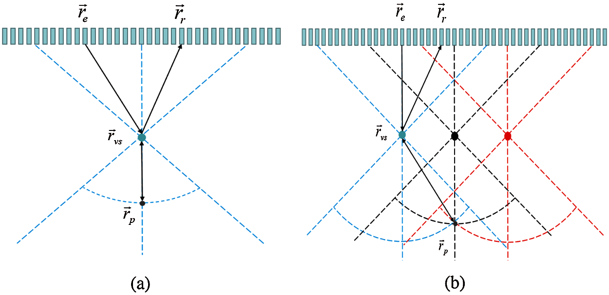
Figure 1: (a) The time-of-flight path for calculation the BF1 receive delay, (b) the ultrasonic field propagation path with sliding sub-aperture

Fig. 1b shows the ultrasonic field propagation path with sliding sub-aperture. Three sub-aperture and three corresponding focuses are marked as VS elements in Fig. 1b. We assume that the image point p located at (x, z) and the focus point located at (xiF,ziF). The propagation time between the image point and the VS is formulated as

ti(x,z)=ziF±(xiF−x)2+(ziF−z)2c(2)

In BF2, each output data is constructed by selecting sample from each LRLs from BF1 which contains information from the spatial position of the image point. Then by summing these samples, results can be obtained. Assuming BF1 output of the point r→p in ith LRL is si(x, z) and from Eq. (2) we can know that si(x, z) = LRL(ti(x, z)). Then, the synthesized signal of the image point is formulated as 1 [3]

H(x,z)=∑i=1I(z)si(x,z)(3)

where H(x, z) is the high resolution image, and I(z) is the number of VS covering the imaging point r→p.

I(z) can be calculated directly from the geometry shown in Fig. 2 as

I(z)=⌊L(z)dΔ⌋=⌊2|z−dv|tan⁡(α2)dΔ⌋(4)

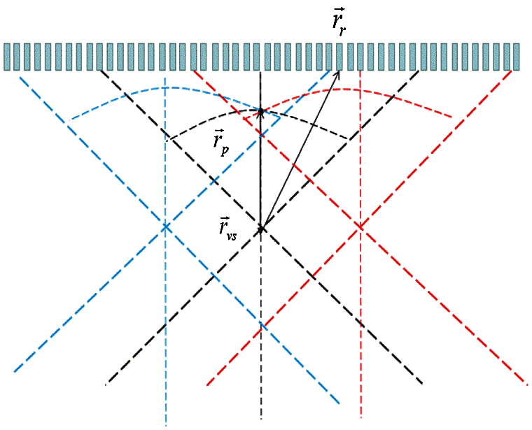
Figure 2: Two consecutive sub-aperture transmit sound field geometry model

where ⌊L(z)dΔ⌋ denotes the largest integer no more than L(z)dΔ. The variable L(z) is the lateral width of the wave field at depth z and dδ is the distance between the VS elements of two continuous emissions. α=2arctan⁡12F is the opening angle of VS. The F-number is F=ZLΔ, where LΔ is the size of sub-aperture.

VS imaging is based on the assumption that the focal region can be seen as the virtual source of a spherical wave within a certain angular range. The VS method can increase lateral resolution and extend imaging depth by combining the adjacent LRLs that contain information of synthesized line.

2.2 Generalized Coherence Factor Weighted VS

From Eq. (3), the traditional VS imaging reconstructs the images without using data characteristics, which results in the wide mainlobe width and high sidelobe level. The GCF weighting method can suppress interfering off-axis scattering signals and allow large sidelobes in directions where no energy is received. It is defined as the ratio of the spectral energy within a pre-specified low-frequency region to the total energy. GCF is respectively represented as

GCF=∑k∈low−frequencyregion|P(k)|2∑k=12N|P(k)|2(5)

where P(k) is the spectrum of the effective sequence LRLs, and 2N is the number of points in the discrete spectrum. The low-frequency region is specified by a cut-off frequency M0 in the spatial frequency index (i.e., from − M0 to M0). In this paper, M0 is set as 3 for GCF. The expression of GCF-weighted VS can be given by

HGCF(x,z)=GCF∑i=1I(z)si(x,z)(6)

2.3 Adjustable Generalized Coherence Factor Weighted VS

GCF can enhance the robustness due to the consideration of the energy of incoherent speckle signals. The performance of GCF is determined by the cut-off frequency M0. The noise reduction and sidelobe suppression capabilities of GCF decrease with the increase of M0, while the background can be further maintained. Thus, aGCF is proposed for VS imaging, in which the value of M0 can be adjusted by SIF.

Fig. 3 shows the schematic of aGCF-VS. We supposed a vector S(x, z) = [s1(x, z), s2(x, z), s3(x, z),…, si(x, z),…, sI(x, z)] and si(x, z) means that the spacial position of imaging point p is located at the ith LRL. We assumed that n = [k, k + 1, k + 2,…, I − k + 1] and the values from sn − k(x, z) to sn + k(x, z) represent effective signal intensity of the point p. The SIF is derived from the vector S(x, z). It is defined as the ratio between the effective echo signals intensity and total intensity.

SIFn(x,z)=∑i=n−kn+k|si(x,z)|∑i=1I|si(x,z)|,k=[I∗m],m=13,14,15,…1I(7)

where m is the effective coefficient, and k is adjusted by m and I. According to statistical properties of the vector S(x, z) derived from the effective field, SIF, which is the mean value of SIFn is proposed as the M0 of GCF. We define this method as aGCF, which can be expressed as

aGCF(x,z)=∑k=−SIFk=SIF|P(k)|2∑k=−Nk=N−1|P(k)|2(8)

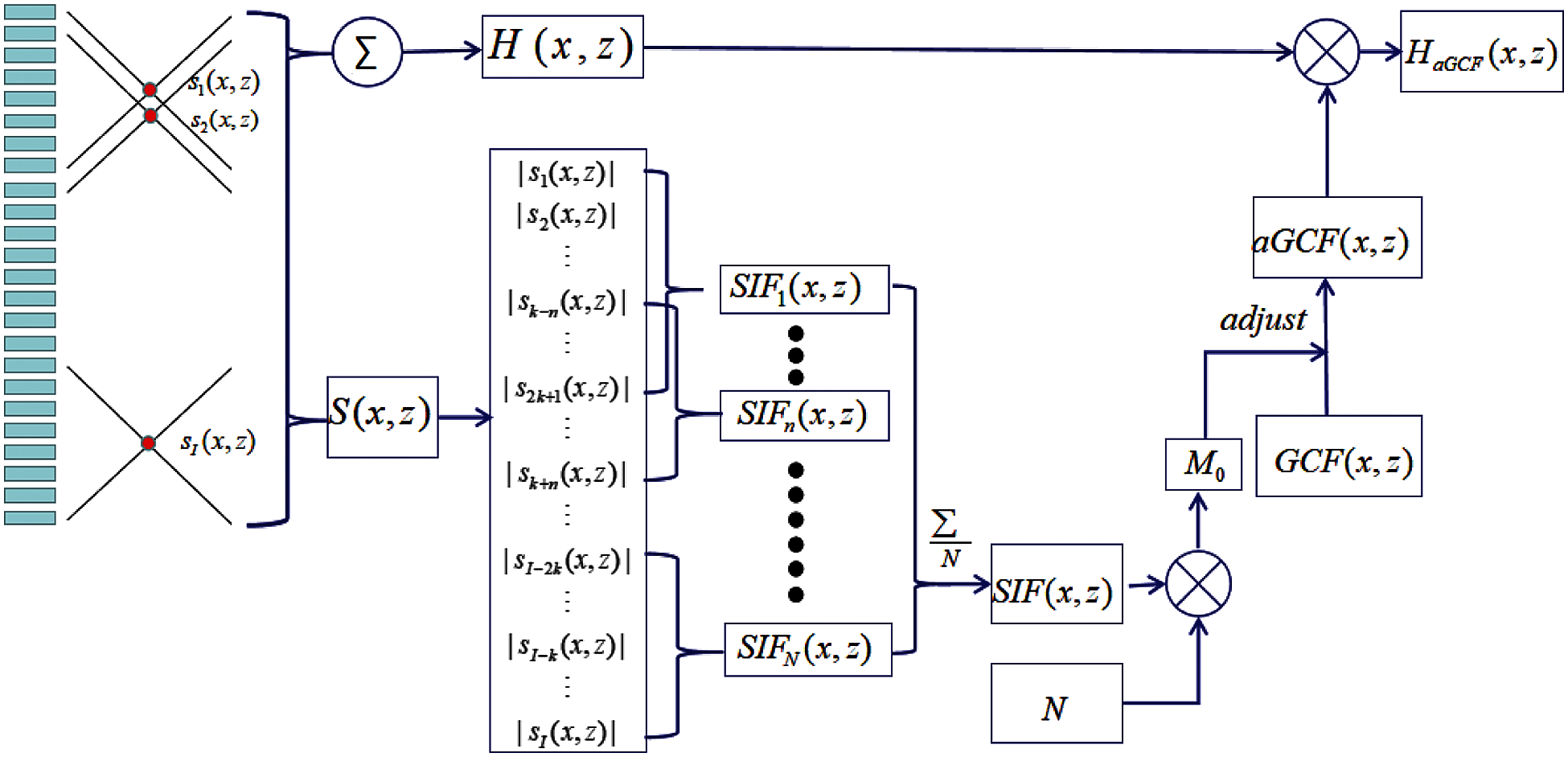
Figure 3: Schematic of the proposed method

As a result, aGCF is introduced into the VS imaging, and the aGCF-VS algorithm can be formulated as

HaGCF(x,z)=aGCF(x,z)∑i=1I(z)si(x,z)(9)

where the HaGCF(x, z) is the high resolution image and si(x, z) is the LRL with the VS at (x, z). If the main signal intensity of point p is noise, the values of SIF(x, z) will be low, and thus the value of aGCF will be lower. aGCF can reduce the noise effectively. If p is the effective scatter points, the elements of S(x, z) seem to be similar and high values. aGCF can avoid overestimating the coherence of scatter point. aGCF is used to weight VS image points to highlight the effective LRLs. Thus, the image quality can be improved.

3  Results

3.1 Simulation and Experimental Setup

In order to verify the performance of the proposed algorithm, aGCF-VS is compared with fixT-fixR imaging, VS imaging and GCF-VS on both simulated and experimental datasets. For aGCF-VS, m values were set to 1/4, 1/6, and 1/8 to show its effect on the image quality.

In simulation, Field II [29,30] was used to generate simulated datasets. A linear array with a pitch of 0.3 mm (element width = 0.25 mm, height = 0.5 mm) was used, which was consisted of 128 elements. The central frequency and the sampling frequency were set to 5 MHz and 150 MHz, respectively. The number of valid elements was set to 64. A 12 mm × 1 mm × 13 mm phantom containing two point targets and a 3 mm radius circular cyst was simulated. Point targets were located at (x, z) = (−3 mm, 15 mm) and (−3 mm, 25 mm). The cyst was centered at (0 mm, 20~mm).

In experiment, the ultrasound imaging system Sonix-Touch (Ultrasonix Medical Corporation, Richmond, BC, Canada), the L14-5 linear array transmitted at 5 MHz and the phantom KS107BD (Chinese Academy of Sciences, China) were used to collect raw channel data sets. The sampling frequency was 40 MHz.

To get a high transmission power, the number of transmit elements is set to 64. In SASB method, grating lobes can be avoided if F-number is no less than 2. As the transducer pitch is equal to 0.3 mm, the focus depth should be set to 40 mm to avoid the effect of grating lobes in simulation and experiment.

3.2 Image Quality Evaluation

For point targets, the full width at half maximum (FWHM, −6 dB mainlobe width) was used as the quantitative indicator of the mainlobe width to evaluate resolution both in lateral and axial directions. To evaluate the improvement in the image contrast and speckle pattern, three common indicators (CR, CNR and sSNR) were measured, which are defined as [31,32]

CR=20 log10|μb||μc|(10)

CNR=|μb−μc|σb+σc(11)

sSNR=|μb|σb(12)

where μb and μc are the mean intensity in the background region and cyst target region respectively, and σb is the standard deviation of the intensity in the background region. The intensity is calculated based on data before log-compress to avoid the effect of dynamic range.

3.3 Simulation Result

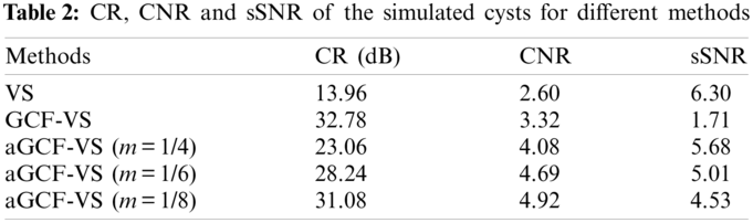
Fig. 4 shows the simulated point images created by different methods over a dynamic range of 60 dB. As seen from Fig. 4, there exist black artifacts beside points in GCF-VS image. Furthermore, it can be seen from Fig. 4c that the noise inside the cyst is less than with other methods. The background brightness of GCF-VS is the lowest. Although the aGCF-VS method has a smaller background brightness than the VS method, it has less noise inside the cyst. Meanwhile, with the appropriate decreases of the m value, the noise level inside the cyst of aGCF-VS decreases significantly.

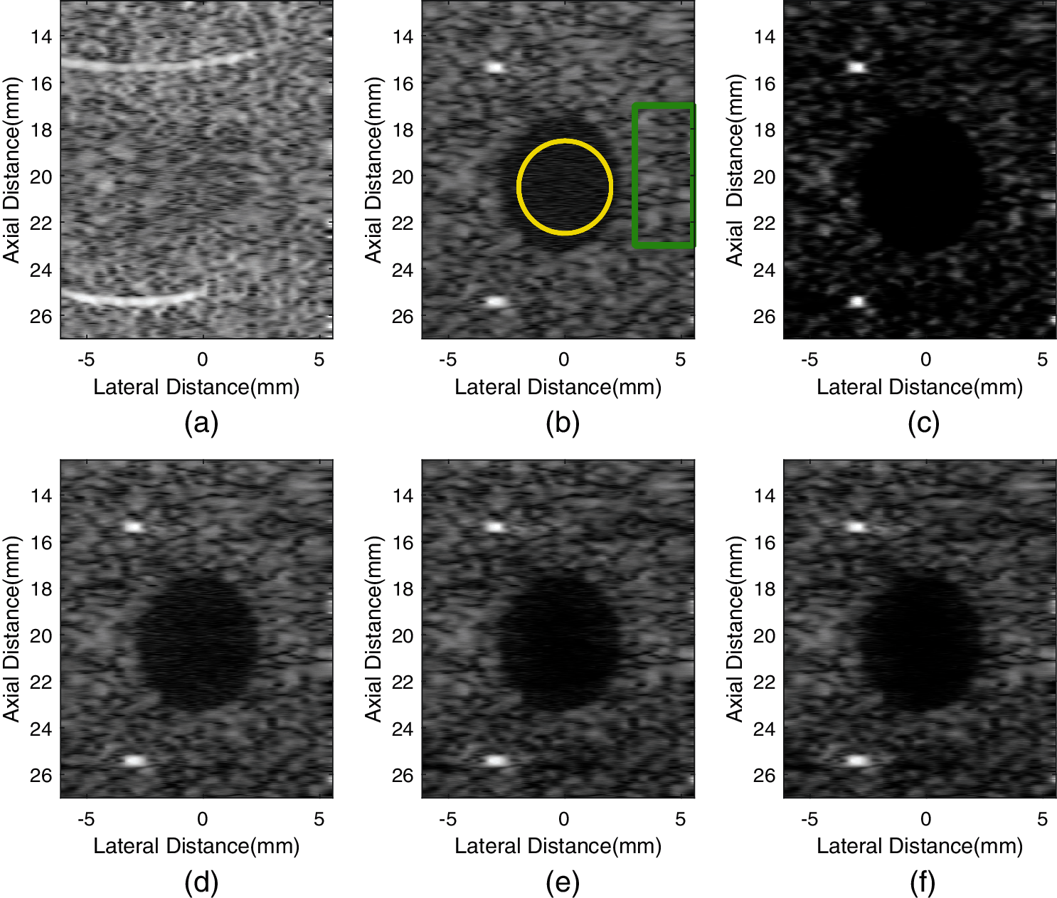
Figure 4: Simulated images formed by different methods. (a) fixT-fixR, (b) VS, (c) GCF-VS, (d) aGCF-VS (m = 1/4), (e) aGCF-VS (m = 1/6), (f) aGCF-VS (m = 1/8)

Fig. 5 shows the lateral and vertical variations of the point targets located at 15 mm depth. We can see that the lateral mainlobes of aGCF-VS methods are similar to that of VS but wider than GCF-VS. Besides, GCF-VS has the narrowest lateral and vertical mainlobe widths, which means that GCF-VS provides a better lateral resolution than other methods.

The quantitative results of FWHM are listed in Table 1. Lateral FWHM of GCF-VS is the smallest, which further demonstrates that GCF-VS can provide the best lateral resolution. Meanwhile, the axial FWHM value of aGCF-VS is smaller than VS. With the variation of m, lateral FWHM of aGCF-VS at 15 mm depth has no significant changes. As a result, it is clear that aGCF-VS can slightly improve the resolution in comparison with VS.

To investigate the contrast of the proposed method for cyst imaging, a circular anechoic cyst is simulated and imaged with these methods. Fig. 4 shows the imaging results of cysts. CR, CNR, and sSNR are calculated for all images and the statistical results are listed in Table 2. It can be seen from Fig. 4 and Table 2 that VS has the highest sSNR but it cannot provide the margin clearly. GCF-VS has the least noise in the cyst. The background intensity of GCF-VS is lower than aGCF-VS and the image of GCF-VS is darker than others. Thus it has the smallest sSNR. In addition, the intensity of VS is higher than GCF-VS and aGCF-VS, which results in high sSNR but poor contrast.

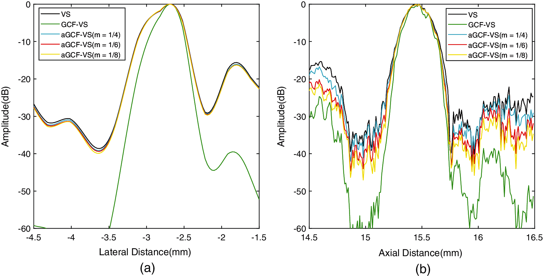
Figure 5: (a) Lateral and (b) axial variations of the simulated point at 15 mm depth

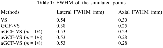
As shown in Table 2, compared with VS, aGCF-VS (m = 1/6) achieves CR and CNR enhancements by 102.3% and 80.2%, respectively. The CNR and sSNR of aGCF-VS (m = 1/6) are increased by 41.5% and 192.7% relative to GCF-VS, but the CR of aGCF-VS (m = 1/6) is decreased by 13.8%. In conclusion, according to the simulation results, in contrast to VS, aGCF-VS can suppress sidelobes and noise. As a result, aGCF-VS has a higher CR than VS. Compared with GCF-VS, aGCF-VS presents higher CNR and sSNR.

3.4 Experimental Result: Point Targets and Cyst Targets

We used the above mentioned methods to analyze experimental data sets collected by Sonix-Touch. All images are displayed over a dynamic range of 60 dB. Fig. 6 shows the experimental point images. We chose a point with a depth of 20 mm for quantitative measurement. The lateral and axial FWHM values are exhibited in Table 3. The variations of the selected point are shown in Fig. 7.

Figure 6: Experimental point images formed by different methods. (a) fixT-fixR, (b) VS, (c) GCF-VS, (d) aGCF-VS (m = 1/4), (e) aGCF-VS (m = 1/6), (f) aGCF-VS (m = 1/8)

Similar to the simulation case, the GCF-VS image of Fig. 6c has the least sidelobes and the background is darker than other images. aGCF-VS can slightly improve the resolution than VS. However, it has a darker background than VS. As the value of m decreases, lateral FWHM of aGCF-VS shows moderate improvement, and there is almost no change in axial resolution. It can also be seen that the background brightness is decreased as the parameter m of aGCF-VS decreases.

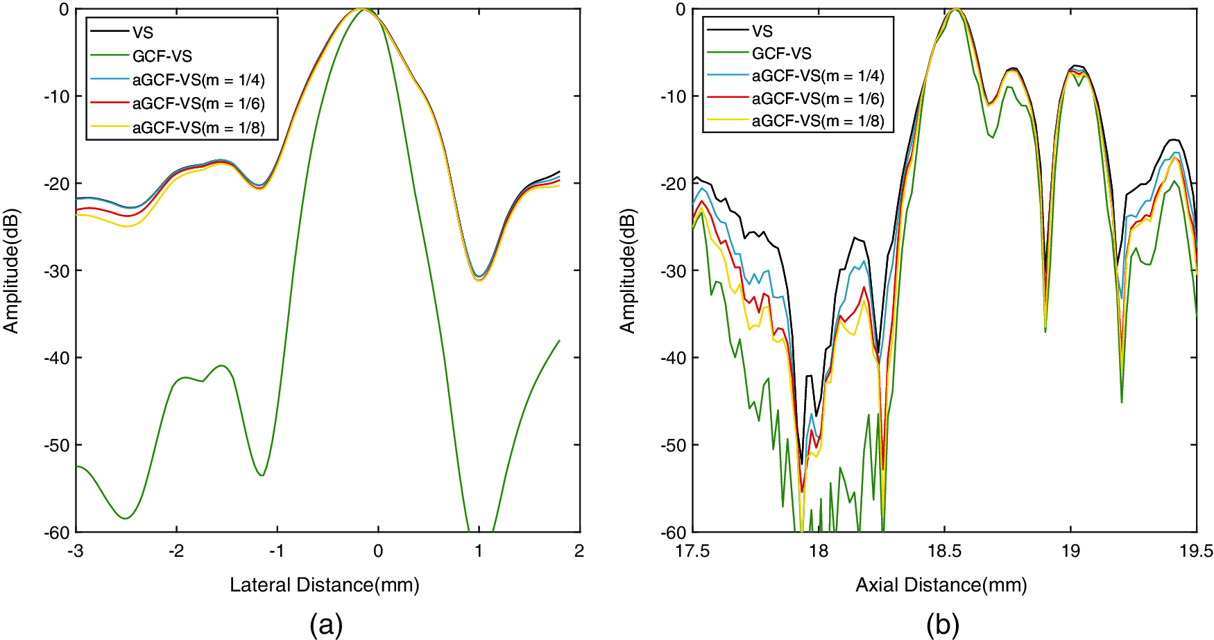
Figure 7: (a) Lateral and (b) axial variations of the experimental point at 20 mm depth

Fig. 8 shows experimental cyst phantom images. The GCF-VS image has lower background intensity than other methods and there are distinct artifacts in background speckle. By adjusting the value of m, the artifacts in the background speckle of the aGCF-VS image are removed. In the aGCF-VS images, not only is the background brightness much better than GCF-VS, but also the contrast between cyst and background is more significant than others.

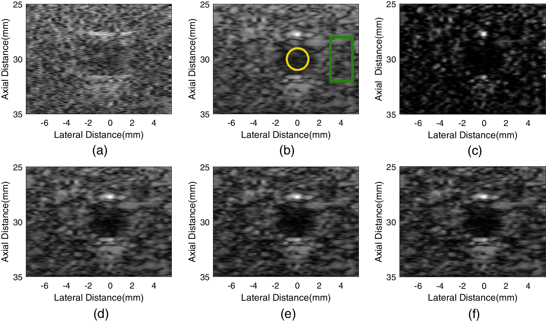
Figure 8: Experimental cyst images formed by different methods. (a) fixT-fixR, (b) VS, (c) GCF-VS, (d) aGCF-VS(m = 1/4), (e) aGCF-VS(m = 1/6), (f) aGCF-VS (m = 1/8)

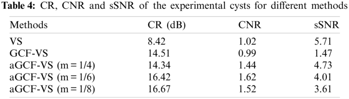
Table 4 displays the CR, CNR and sSNR values of the cyst. In comparison with VS, the CR and CNR of aGCF-VS (m = 1/6) are increased by 95.0% and 60.8%. The CR and CNR of aGCF-VS (m = 1/6) are improved by 13.2% and 63.6% relative to GCF-VS, and the sSNR of aGCF-VS (m = 1/6) is improved by 173.8%. From Table 4, the experimental results are almost consistent with the simulation results.

3.5 In-Vivo Human Carotid Artery Images

For the in-vivo experiment, echo signals from the transverse cross section of a human carotid artery were collected to evaluate the proposed method. The results are shown in Fig. 9. The CR, CNR, and sSNR values are given in Table 5.

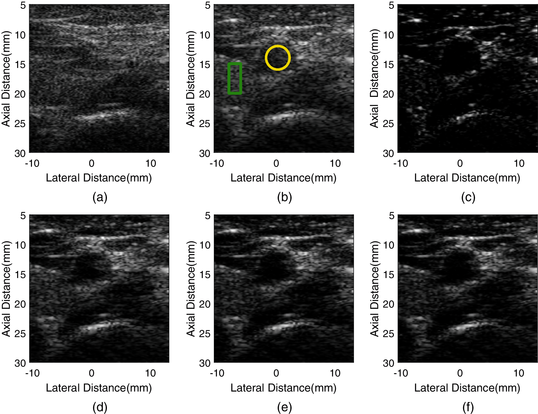
Figure 9: The images of human carotid artery formed by different methods. (a) fixT-fixR, (b) VS, (c) GCF-VS, (d) aGCF-VS (m = 1/4), (e) aGCF-VS (m = 1/6), (f) aGCF-VS (m = 1/8)

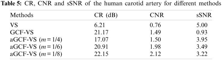
Compared with VS, aGCF-VS shows improved image quality, in which the aGCF-VS method reduces noise and provides clearer boundary of the carotid artery. aGCF-VS also provides more preserved anatomical structures than GCF-VS. Besides, hyperechoic structures are more distinct, and the hypoechoic tissue inside the artery is less visualized. Meanwhile, the anatomical structures around the artery of aGCF-VS are more visible. In Table 5, in comparison with VS, aGCF-VS (m = 1/6) offers CR and CNR enhancements of 236.7% and 160.5%. aGCF-VS (m = 1/6) can obtain increased CNR and sSNR by 32.9% and 275.3% than GCF-VS, respectively. Thus, the aGCF-VS method can be used for biological tissue imaging with improved image quality.

4  Discussion

This paper proposes aGCF to weight VS for the image quality improvement in ultrasound imaging. Simulation and experimental results demonstrate that aGCF-VS can reduce the noise. This is because that SIF in aGCF utilizes a significant part of LRLs. Besides, aGCF-VS is more effective in maintaining the background intensity than GCF-VS.

It can be seen from Figs. 4 and 6, GCF-VS has a better resolution than VS. The GCF-VS provides the narrowest mainlobe. The superiority of GCF-VS is due to the suppression of off-axis incoherent signals. This is because these weighting factors utilize the statistical properties of received signals and highlight the effective LRLs which contain the sidelobe signal strength of the adjacent area. According to Eqs. (4) and (9), the SIF value that replaces the cut-off frequency M0 will not be small, so compared to DAS, the resolution of aGCF is not much improved.

As illustrated in Tables 2 and 4, for cyst imaging, the weighted VS methods can significantly enhance the image contrast. However, the GCF-VS algorithm cannot protect the background speckle pattern and it degrades the speckle brightness, which results in a decreased sSNR. Furthermore, the GCF-VS algorithm introduces black artifacts and severely reduces the uniformity of the background. This is because the background speckle has both coherent and incoherent components, and when the cut-off frequency M0 of GCF is set to a small value, only the coherent part of the signal remains. The results in Figs. 4 and 8 show that aGCF has can suppress noise, and thus enhance contrast. This is due to highlighting the effective LRLs in aGCF. Besides, as aGCF can protect the incoherent signals in the background, it can preserve the speckle pattern. So aGCF-VS can provide higher speckle brightness, higher CNR and sSNR than GCF-VS. As shown in Fig. 9 and Table 5, aGCF-VS can provide better carotid artery images and the in-vivo images have better robustness than GCF-VS. Therefore, aGCF used to weight the VS images has the potential to suppress artifacts and obtain high quality images. In addition, the resolution changes slightly as the m value decreases.

The value of m has an impact on the performance of aGCF-VS. We observe that aGCF can show difference in performance in reducing the speckle artifacts and improving background brightness by adjusting the m value. To further illustrate the proposed method, quantitative values of CR, CNR and sSNR of simulated phantom images formed by aGCF-VS with different m values (1/4, 1/6, 1/8, 1/10, 1/12) are calculated. As seen from Fig. 10, as the value of m decreases, CR and CNR gradually increase, while sSNR gradually decreases. Considering the overall quality of the image, m = 1/8 is recommended for aGCF-VS to obtain high quality images.

The computational complexity of GCF and SIF is O(2 Nlog2N) and O(I), respectively. Therefore, the computational complexity of aGCF is the same as GCF. However, the computational load of aGCF is more than GCF, since the SIF requires (2k + 1 + I) × (I − 2k + 1) additions and I absolute operations.

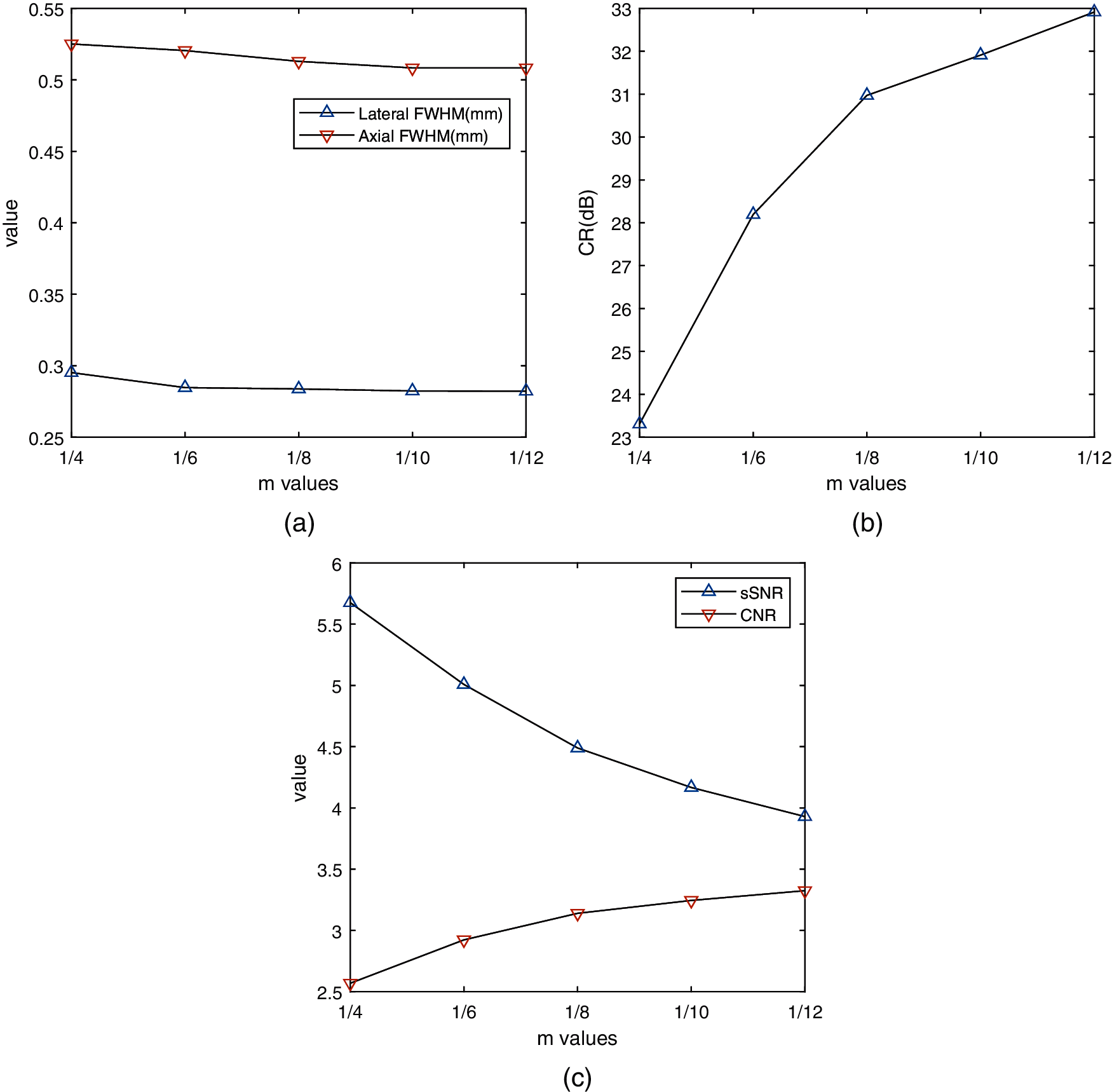
Figure 10: The values of image metrics with different m values in simulation phantom images with aGCF-VS method. (a) FWHM, (b) CR, (c) CNR and sSNR

5  Conclusion

We have studied the combination of the VS imaging method and aGCF weighting algorithm for medical ultrasound imaging. Simulation and experiments were conducted to study the performance of the proposed method. Results demonstrated the effectiveness of the proposed method to improve image quality for ultrasound imaging. aGCF can improve contrast and maintain the speckle pattern with low computational complexity. We studied the different values of m. It is suggested that m should be set to 1/8 so that the CR and CNR could be improved while obtaining enhanced sSNR. Due to the effective improvement of speckle quality and low computational complexity in our method, it is beneficial to reduce the performance requirements of ultrasound medical imaging equipment, thereby reducing commercial manufacturing costs, while the image quality can also be guaranteed. Thus it has the potential to be implemented in a commercial system to enhance the image quality. Finally, the major challenge in the current study is the limited resolution. Our future study will optimize the proposed method to improve the lateral resolution.

Funding Statement: The National Natural Science Foundation of China (Grant No. 62071165), the Fundamental Research Funds for the Central Universities of China (Grant No. JZ2021HGTB0074), the China Postdoctoral Science Foundation (Grant No. 2021M690853).

Conflicts of Interest: The authors declare that they have no conflicts of interest to report regarding the present study.

This work is licensed under a Creative Commons Attribution 4.0 International License, which permits unrestricted use, distribution, and reproduction in any medium, provided the original work is properly cited.