| Computer Modeling in Engineering & Sciences |
DOI: 10.32604/cmes.2022.017714
ARTICLE
A New Rayleigh Distribution: Properties and Estimation Based on Progressive Type-II Censored Data with an Application
Department of Statistics, Faculty of Science, King Abdulaziz University, Jeddah, Saudi Arabia
*Corresponding Author: Abdullah M. Almarashi. Email: abdmmar1975@gmail.com; aalmarashi@kau.edu.sa
Received: 31 May 2021; Accepted: 04 August 2021
Abstract: In this paper, we propose a new extension of the traditional Rayleigh distribution called the modified Kies Rayleigh distribution. The new distribution contains one scale and one shape parameter and its hazard rate function can be increasing and bathtub-shaped. Some mathematical properties of the new distribution are derived including quantiles and moments. The parameters of modified Kies Rayleigh distribution are estimated based on progressively Type-II censored data. For this purpose, we consider two estimation methods, namely maximum likelihood and maximum product of spacing estimation methods. To compare the efficiency of the proposed estimators, a simulation study is carried out. To show the applicability of the new model as well as the estimation methods, one real data for failure times of software is analyzed. Based on the empirical parts, we can conclude that the proposed model can be considered as a good model in the field of life testing and reliability analysis compared with other competing models.
Keywords: Rayleigh distribution; modified kies family; progressive Type-II censored; maximum likelihood estimation; maximum product of spacing
The Rayleigh distribution was originally introduced by [1] to study problems in acoustics and optics fields. It has a strong modeling ability of positive skewed data gathered from many fields such as life sciences, reliability analysis and engineering. Moreover, It has gained a great attention from engineers and physicists to model radiation, synthetic aperture radar images, and wave propagation. The Rayleigh distribution can be considered as a special case from two-parameter Weibull distribution with shape parameter equals two. The hazard rate function of the Rayleigh distribution is an increasing failure rate which makes it a good choice to model data with age rapidly over time. The probability density function (PDF) of the Rayleigh distribution is given by
and the corresponding cumulative distribution function (CDF) is
where θ is a scale parameter. It has a disadvantage since the distribution has only a scale parameter and this makes the distribution is not able to model various hazard rate shaped. The need for a new modification to the Rayleigh distribution is still an attractive topic to overcome this disadvantage. Many authors introduced a new generalizations to the Rayleigh distribution, see for example, generalized Rayleigh distribution proposed by [2], beta generalized Rayleigh distribution by [3], transmuted Rayleigh distribution by [4], slashed exponentiated Rayleigh distribution by [5], Weibull Rayleigh distribution by [6], Marshall-Olkin extended generalized Rayleigh distribution by [7] and Slashed generalized Rayleigh distribution by [8]. Recently, the estimation of parameters for some generalizations of Rayleigh distribution under censoring schemes is very common [9] studied the generalized Rayleigh distribution based on a progressive Type-II censored data [10] considered estimation of parameters of an inverted exponentiated Rayleigh distribution based on Type II progressive censored data [11] considered the problem of estimating parameters of the inverted exponentiated Rayleigh distribution based on adaptive Type II progressive hybrid censored data.
Recently, based on the T-X family pioneered by [12], Al-Babtain et al. [13] proposed a new generalized family of continuous distributions called modified Kies generalized (MKi-G) family. Let G(x;ψ) is the baseline CDF with parameter vector ψ, then the CDF and the PDF of the MKi-G family are given, respectively, by
and
They studied the main properties of the MKi-G family and applied it to generate a new extension of the exponential distribution which called modified Kies exponential (MKEx) distribution. Based on the data analysis, they proved that this distribution is a good competitive model to some well-known distribution.
The main aim of this paper is to introduce a new flexible extension of the Rayleigh distribution based on the MKi-G family of distribution by putting the CDF of Rayleigh distribution given by Eq. (2) as a baseline in Eq. (3). We referred to the new distribution as modified Kies Rayleigh (MKR) distribution which contains one scale and one shape parameter. We discuss some properties of the MKR distribution including quantile function, moments and order statistics. Our motivation to consider the MKR distribution is based on its flexible and simple PDF which can be considered to model positive skewed data. It is also capable of modeling monotonically increasing and bathtub shaped. Another motivation of this paper is empirical based. We show later, based on analyzing real data that the MKR distribution outperforms some of the well-known two-parameter distributions as Weibull and gamma distributions. Furthermore, we use the maximum likelihood and maximum product of spacing estimation methods to estimate the parameters of the MKR distribution based on progressive Type-II censored (PT-IIC) data. We provide a guideline for selecting the best estimation method which may be of a great interest to reliability engineers and applied statisticians.
The rest of this paper is organized as follows: The MKR distribution is considered in Section 2. The main properties of the new distribution are discussed in Section 3. Section 4 introduces the maximum likelihood and maximum product of spacing estimation based on PT-IIC sample. In Section 5 we perform a simulation study to compare the different estimators. One real data set for failure times of software is analysed in Section 6. Finally, in Section 7 the paper is concluded.
By inserting G (x;θ) of the Rayleigh distribution given by Eq. (2) in Eq. (3), one can obtain the CDF of the MKR distribution as follows:
where θ and α are the scale and shape parameters, respectively. Similarity, the PDF of the MKR distribution can be obtained by inserting Eqs. (1) and (2) in Eq. (4) as
The reliability function (RF) and the hazard rate function (HRF) of the MKR distribution are, respectively, given by
and
Fig. 1 displays the different plots of the PDF of the MKR distribution using θ = 1 in all the cases with different values for the shape parameter α. From Fig. 1 we can observe that the new shape parameter provides more flexibility to the PDF of the MKR distribution than the traditional Rayleigh distribution with only one scale parameter. It is also noted that the new distribution is able to fit a unimodal or bimodal data. Fig. 2 presents the different shapes of the HRF of the MKR distribution. Fig. 2 shows that the MKR distribution is useful in modeling increasing hazard rate or bathtub-shaped hazard rate.
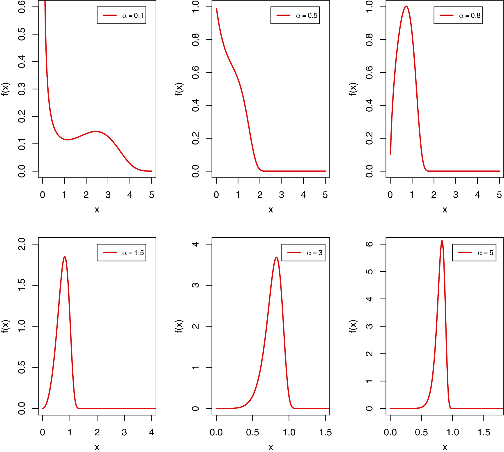
Figure 1: Various plots of the PDF of the MKR distribution for different values of α with θ = 1
3 Mathematical Properties of the MKR Distribution
In this section, the main mathematical properties of the MKR distribution are derived including quantile function, mixture representation and moments.
The quantile function (QF) of the MKR distribution can be obtained by inverting the CDF in Eq. (5) as
By setting q = 0.5 in Eq. (9), one can obtain the median of the MKR distribution in the form
Using the same approach the first and third quartiles of the MKR distribution can be obtained from Eq. (9) by setting q = 0.25 and 0.75, respectively. Another important use to the QF in Eq. (9) is to generate the random variate of the MKR distribution. We can simulated a random sample of size n from the MKR distribution as follows:
where ui is generated from the Uniform (0, 1) distribution.
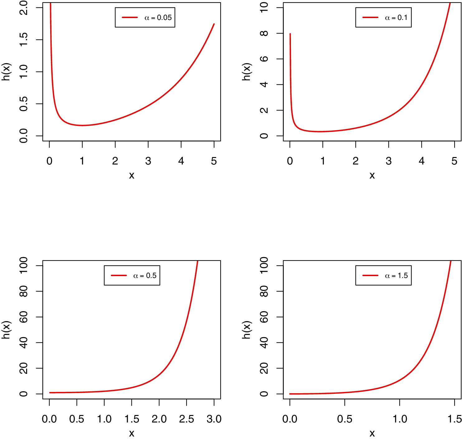
Figure 2: Various plots of the HRF of the MKR distribution for different values of α with θ = 1
The mixture representation of the PDF in Eq. (6) is very useful to derive the main properties of the MKR distribution directly from Rayleigh distribution. Based on Eq. (6) and using the exponential expansion of the term
By expanding the binomial term in Eq. (11) we can obtain
After some simplifications, the mixture representation of the PDF of the MKR distribution can be written as follows:
where
3.3 Moments and Moment Generating Function
Moments are useful to obtain the properties of a distribution including mean, variance, skewness and kurtosis. Let Z be a random variable following the Rayleigh distribution with scale parameter θ. Then the raw moments and the moment generating function of Z are, respectively given by
and
The rth moments of the MKR distribution follows from Eq. (13) as
where follows the Rayleigh distribution with scale parameter θ[j − α (k + 1)]. Then, using the moment of Y given by Eq. (14) and substituting in Eq. (16) we can obtain
Eq. (17) can be used to obtain the first four moments of the MKR distribution and in turn to obtain the variance, skewness and kurtosis using a well-known relations. Following the same approach, the moment generating function of the MKR distribution can be obtained from Eqs. (13) and (15) as
Fig. 3 displays the different plots of the mean, variance, skewness and kurtosis of the MKR distribution obtained using Eq. (17) using different values to the shape parameter α with scale parameter one in all the cases. It is noted from Fig. 3 that the mean and variance of the MKR distribution decrease as the shape parameter α increases. As α increases the skewness decrease at first then increases. Also, it is observed that the kurtosis increases as α increase.
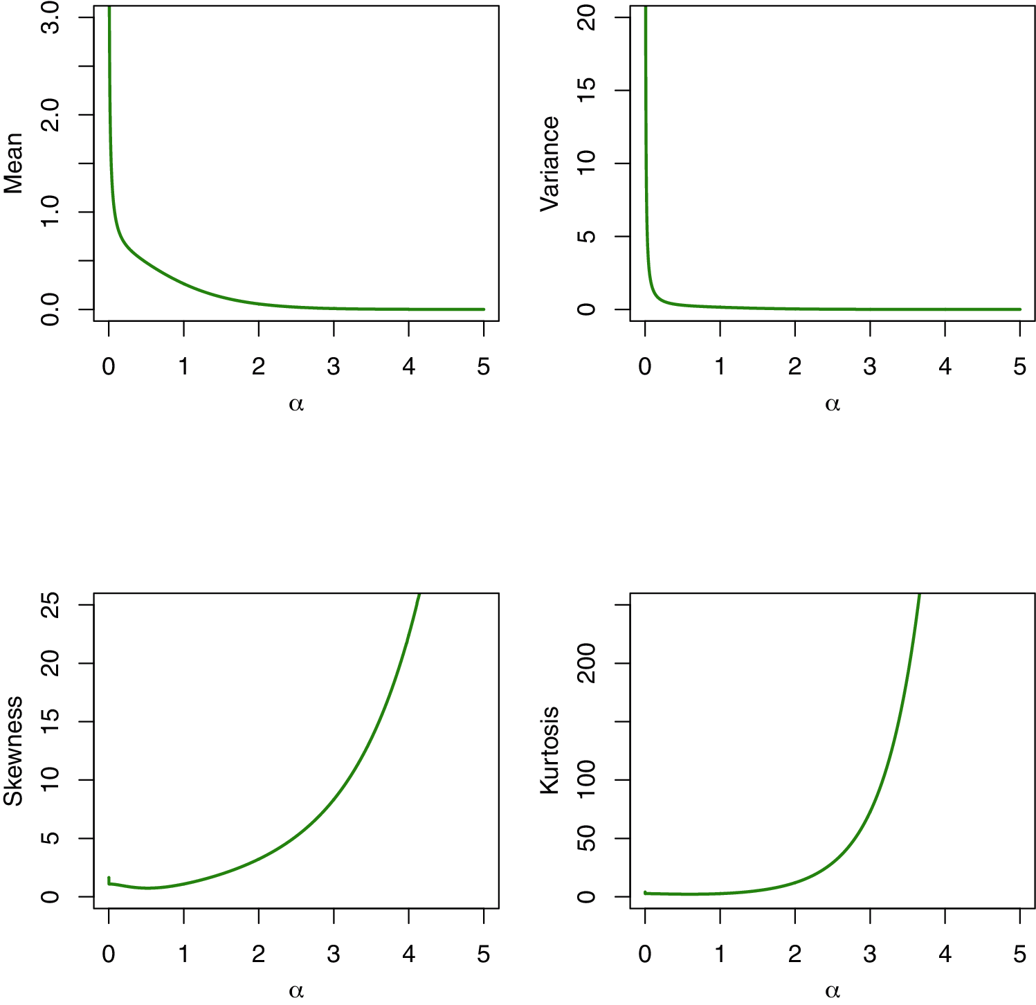
Figure 3: Mean, variance, skewness and kurtosis of the MKR distribution
Let X1:n,…,Xn:n be the order statistics of a random sample obtained from a continuous distribution. The PDF and CDF of the jth order statistic of Xj:n are defined, respectively, as
and
where
Using the binomial expansion in Eq. (21) follows:
where
Expanding the last term in Eq. (24) follows:
where
4 Parameter Estimation under PT-IIC Sample
Censoring is a very common phenomenon in life testing and reliability analysis. Censoring implies that exact failure times are known for only a part of the items under study. There are several censoring schemes in the literature, and the most common ones are Type-I and Type-II censoring. In the Type-I censoring the test is terminated at a prefixed time while in the Type-II censoring the test is terminated when exact units fail. Many authors investigated the estimation problems under these schemes [14] obtained the estimates of the Weibull distribution in the presence of Type-I censored data [15] investigated the Bayesian inference and prediction of the inverse Weibull distribution based on Type-II censored data [16] discussed the Bayesian estimation and prediction using Type-II censored data for the Weibull distribution [17] studied the statistical inference and prediction for Burr Type XII distribution under Type II censored data. Due to rapid advancement in technology, experimenters often want to decrease the total testing time and cost. Therefore, a very flexible and general censoring scheme called the PT-IIC scheme was introduced in practice. In PT-IIC scheme, n units are put on a life test with a prefixed progressive censoring scheme
4.1 Maximum Likelihood Estimation
Let
Substituting Eqs. (5) and (6) in Eq. (25) and taking the natural logarithm, the log-likelihood function can be obtained as
where xi = xi:r for simplicity. The maximum likelihood estimates (MLEs) of the parameters α and θ can be obtained by solving the two normal equations simultaneously. The two normal equations are obtained from Eq. (26) as follow:
and
It is observed from Eqs. (27) and (28) that there are no closed forms for the MLEs of α and θ, denoted by
4.2 Maximum Product of Spacings Estimation
Cheng et al. [24] introduced the method of maximum product of spacings as a good alternative to the method of maximum likelihood. The maximum product of spacings estimates (MPSEs) are obtained by selecting the parameter values that maximize the product of the distances between the values of the distribution function at adjacent ordered points. For PT-IIC data [25] wrote the product of spacing function to be maximized in the following form:
From Eqs. (5) and (29), we can write the natural logarithm of the product of spacing function as follows:
The MPSEs of α and θ, denoted by
and
where
In this section, we present some simulation results to compare the behaviour of the MLEs and MPSEs explained in the previous section. In order to compare the performance of the different estimates we consider to use the mean relative estimates (MREs) and the mean squared errors (MSEs). Based on this approach, the most efficient estimate is expected to has MRE tending to 1 and MSEs approaching to 0 as the effective number of failures r increases. The simulation study involve the following steps:
(1) Determine the values of
(2) Generate the PT-IIC sample using the approach proposed by [26] as follows:
(a) Simulate Y from uniform (0, 1).
(b) Set
(c) Set Ui = 1 − VrVr−1…Vr−i+1 for
(d) Set
(3) Compute the MLEs and MPSEs of α and θ.
(4) Repeat Steps 2–3 M times.
(5) Obtain the average values of MREs and MSEs as follow
where β1 = α and β2 = θ.
The simulation results are obtained based on 1000 PT-IIC generated samples from MKR distribution of sizes (n, r) = (20, 5), (30, 5), (30, 10), (60, 10), (60, 15), (60, 20) and (120, 40). We use three sets of the parameters values, (α,θ) = (2, 2), (1.5, 3) and (3, 1.5). Also, the MLEs and MPSEs are obtained by using three progressive censoring schemes (Schs). Sch 1:
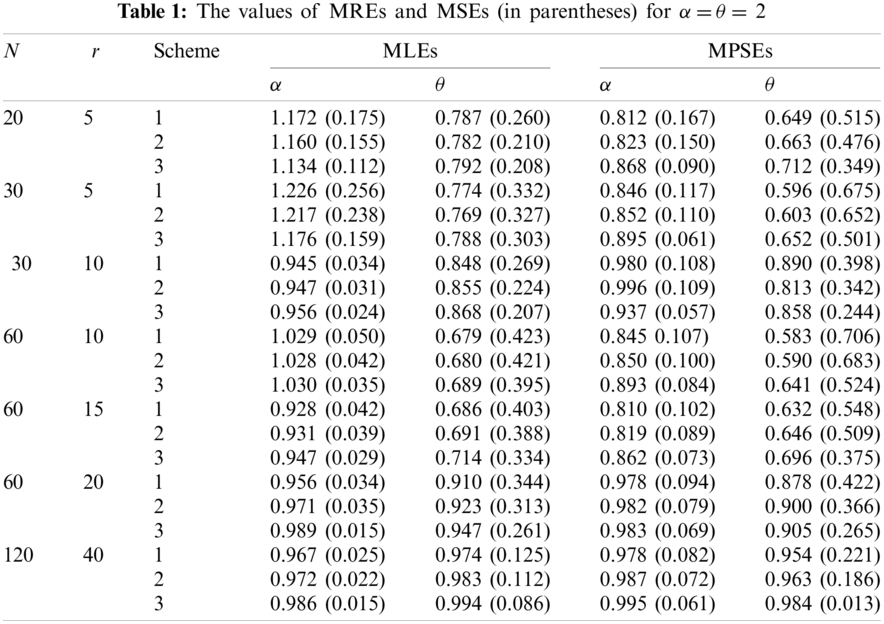
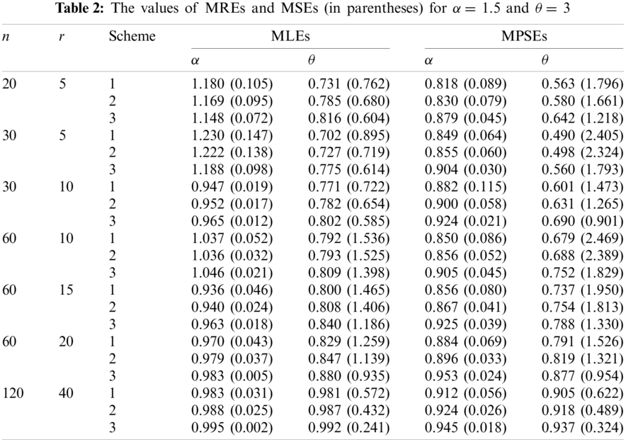
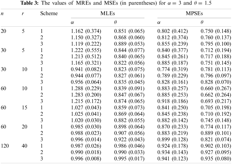
From these Tables we can conclude the following:
1. The values of MREs approach to one as r increases using the both estimation methods, which implies that the MLEs and MPSEs are consistent.
2. The values of MSEs tend to zero as r increases using the both estimation methods, which implies that the MLEs and MPSEs are asymptotically unbiased.
3. The results of Sch 3 perform better than the other two schemes based on minimum MSEs for the two parameters.
4. The MREs of the MLEs are closer to one than those based on MPSEs.
5. The MLEs perform better than the MPSEs in terms of minimum MSEs.
Based on the above results and taking into account the attractive properties of MLEs, we can conclude that the maximum likelihood method can be superiorly preferred to estimate the parameters of the MKR distribution.
In this section, we consider one real data set (DS) to see the applicability of the MKR distribution as well as the different estimation methods. The real DS is given by [27]. The original DS consists of sixteen observations and presents the failure times of the release of software given in terms of hours with average life time be 1000 h from the starting of the execution of the software. Table 4 displays the complete DS. We use the MLEs to check the suitability of the MKR distribution to fit this DS. The Kolmogorov-Smirnov (K-S) distance and the corresponding p-value are displayed also in Table 4. Based on K-S and the associated p-value we can conclude that the MKR distribution is an acceptable model to fit the DS. The total time test (TTT) plot is a graphical technique to show whether the data can be applied to a specific distribution or not. According to Aarset [28] the HRF is constant if the TTT plot is graphically presented as a straight diagonal. On the other hand, the HRF is increasing if the TTT plot is concave and it is decreasing if the TTT plot is convex. Fig. 4 displays the TTT plot of the DS which indicates that the empirical hazard function of this data is increasing. Therefore, the MKR distribution is suitable to model the DS.
We use the DS to compare the MKR distribution with some well-known competitive models with two parameters, namely, Weibull (We), MKEx by Al-Babtain et al. [13], exponentiated Rayleigh (ER), which is also called generalized Rayleigh, exponentiated exponential (EEx), gamma (Ga) distributions. In all the mentioned models we consider α and θ to be the shape and scale parameters, respectively. It is to be mentioned here that these models are selected because they have the same number of parameters similar to the MKR model as well as they have the ability to model increasing HRF. The MLEs of the different models with the associated standard errors are obtained and tabulated in Table 5. To compare the fit of the different models, the negative of the log-likelihood function (L) and the K-S and the corresponding p-values are also obtained and presented in Table 5. Moreover, the Akaike information criterion (AIC); AIC = 2p − 2L, consistent Akaike information criterion (CAIC); ACIC = AIC + 2p(p + 1)/(n − p − 1), and Bayesian information criterion (BIC); BIC = plog(n) − L, where p is the number of the unknown parameters, are obtained to compare the fit of the different models. These values are displayed in Table 5. Based on the results in Table 5, it is noted that the MKR model has the smallest-L, AIC, CAIC, BIC and K-S with the largest p-value when comparing with other models. Therefore, we can say that the MKR distribution is the best model to fit this DS. The estimated CDF, RF, PP and HRF plots of the MKR distribution are presented in Fig. 5. The plots in Fig. 5 indicate that the MKR distribution is suitable for modeling the given DS.
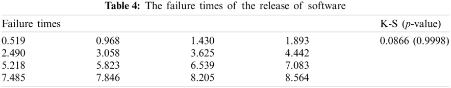
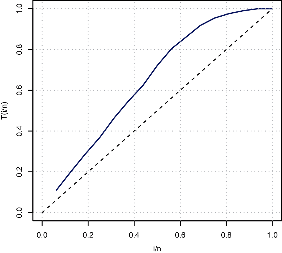
Figure 4: TTT plot of DS
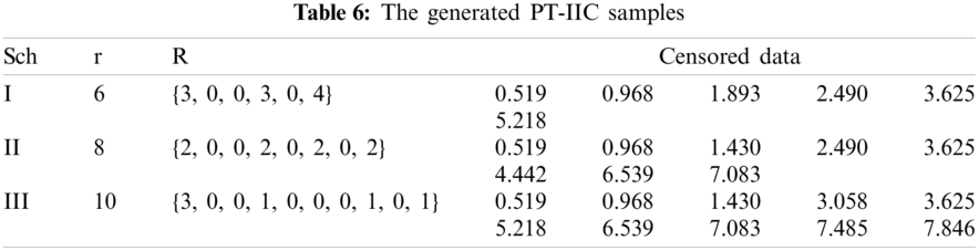
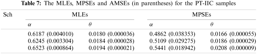
To estimate the parameters of the MKR distribution based on PT-IIC scheme we consider to use the same PT-IIC samples used by [20] and generated from the original DS displayed in Table 4. Dey et al. [20] generated three PT-IIC samples with different schemes as presented in Table 6. Using the generated PT-IIC samples in Table 6, the MLEs and MPSEs are obtained and displayed in Table 7. In addition, the approximated MSEs (AMSEs) are computed by assuming that the MLEs based on the complete DS as the true parameter values. The values of AMSEs are displayed also in Table 7. The results in Table 7 indicate that the MLEs perform better than the MPSEs in terms of AMSEs except the case when estimating the parameter θ using Sch 3. Also, it is observed that the MLEs and MPSEs using Sch 3 have the smallest AMSEs comparing with those based on Schs 1 and 2. The analysis of the real DS indicates the importance of the proposed MKR distribution in the field of life testing and reliability analysis comparing with some other competitive models including Weibull and gamma distributions.
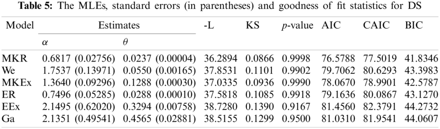
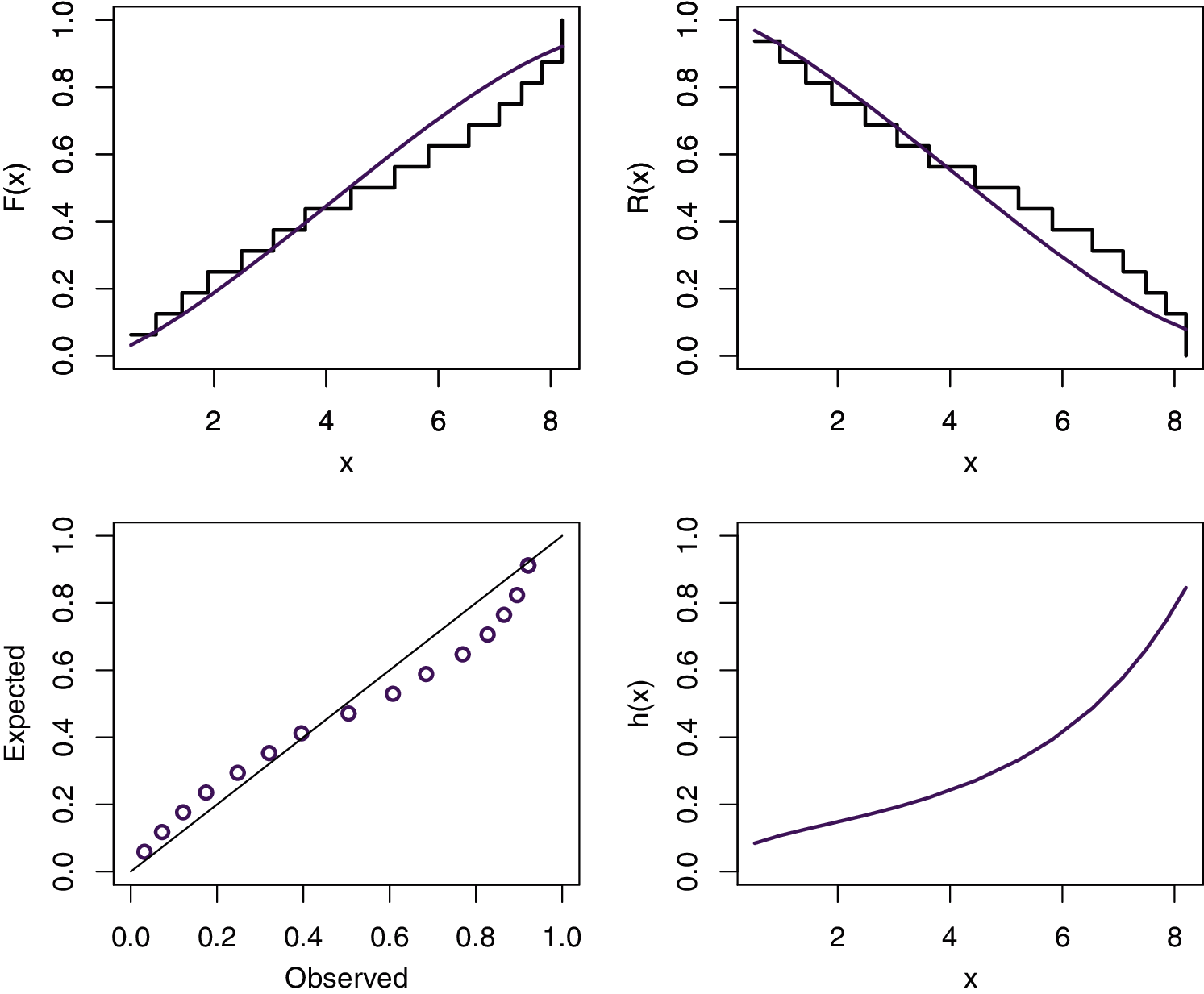
Figure 5: Estimated CDF, RF, PP and HRF plots of the MKR distribution for data DS
In this paper, we have introduced a new lifetime model called the modified Kies Rayleigh (MKR) distribution. The MKR distribution has one scale and one shape parameter. Its hazard rate function can be monotonically increasing and bathtub shaped. Some mathematical properties of the MKR distribution are derived including quantiles, moments and order statistics. The unknown parameters of the proposed distribution are estimated based on progressively Type-II censoring data. The parameters are estimated by considering the maximum likelihood and maximum product of spacing estimation methods. To compare the performance of these estimators, a simulation study is conducted by considering different parameter values and schemes. The simulation results showed that the maximum likelihood estimates perform better than those based on maximum product of spacing method in terms of mean squared error. As an application, one real data set for failure times of software is considered. The real data analysis showed that the MKR distribution is a good model to fit this data and provides a better fit rather than some other competitive models with two-parameters as Weibull and gamma distributions.
Acknowledgement: The authors would like to thank the Editorial Board and reviewers for their valuable comments that greatly improved the final version of the paper.
Funding Statement: This project was funded by the Deanship Scientific Research (DSR), King Abdulaziz University, Jeddah under Grant No. (G:337-130-1441). The authors, therefore, acknowledge with thanks DSR for technical and financial support.
Conflicts of Interest: The authors declare that they have no conflicts of interest to report regarding the present study.
1. Rayleigh, L. (1880). On the stability or instability of certain fluid motions. Proceedings of London Mathematical Society, 1(1), 57–70. London. DOI 10.1112/plms/s1-11.1.57. [Google Scholar] [CrossRef]
2. Surles, J., Padgett, W. (2001). Inference for reliability and stress-strength for a scaled burr type x distribution. Lifetime Data Analysis, 7(2), 187–200. DOI 10.1023/A:1011352923990. [Google Scholar] [CrossRef]
3. Cordeiro, G. M., Cristino, C. T., Hashimoto, E. M., Ortega, E. M. (2013). The beta generalized Rayleigh distribution with applications to lifetime data. Statistical Papers, 54(1), 133–161. DOI 10.1007/s00362-011-0415-0. [Google Scholar] [CrossRef]
4. Merovci, F. (2013). Transmuted Rayleigh distribution. Austrian Journal of Statistics, 42(1), 21–31. DOI 10.17713/ajs.v42i1.163. [Google Scholar] [CrossRef]
5. Salinas, H. S., Iriarte, Y. A., Bolfarine, H. (2015). Slashed exponentiated Rayleigh distribution. Revista Colombiana de Estadstica, 38(2), 543–466. DOI 10.15446/rce.v38n2.51673. [Google Scholar] [CrossRef]
6. Merovci, F., Elbatal, I. (2015). Weibull Rayleigh distribution: Theory and applications. Applied Mathematics and Information Sciences, 9(4), 2127–2137. DOI 10.12785/amis/090452. [Google Scholar] [CrossRef]
7. MirMostafaee, S. M. T. K., Mahdizadeh, M., Lemonte, A. J. (2017). The marshall-olkin extended generalized Rayleigh distribution: Properties and applications. Communications in Statistics-Theory and Methods, 46(2), 653–671. DOI 10.1080/03610926.2014.1002937. [Google Scholar] [CrossRef]
8. Iriarte, Y. A., Vilca, F., Varela, H., Gómez, H. W. (2017). Slashed generalized Rayleigh distribution. Communications in Statistics-Theory and Methods, 46(10), 4686–4699. DOI 10.1080/03610926.2015.1066811. [Google Scholar] [CrossRef]
9. Raqab, M. Z., Madi, M. T. (2011). Inference for the generalized Rayleigh distribution based on progressively censored data. Journal of Statistical Planning and Inference, 141(10), 3313–3322. DOI 10.1016/j.jspi.2011.04.016. [Google Scholar] [CrossRef]
10. Rastogi, M. K., Tripathi, Y. M. (2014). Estimation for an inverted exponentiated Rayleigh distribution under Type II progressive censoring. Journal of Applied Statistics, 41(11), 2375–2405. DOI 10.1080/02664763.2014.910500. [Google Scholar] [CrossRef]
11. Panahi, H., Moradi, N. (2020). Estimation of the inverted exponentiated Rayleigh distribution based on adaptive Type II progressive hybrid censored sample. Journal of Computational and Applied Mathematics, 364, 112345. DOI 10.1016/j.cam.2019.112345. [Google Scholar] [CrossRef]
12. Alzaatreh, A., Lee, C., Famoye, F. (2013). A new method for generating families of continuous distributions. Metron, 71, 63–79. DOI 10.1007/s40300-013-0007-y. [Google Scholar] [CrossRef]
13. Al-Babtain, A., Shakhatreh, A. M. K., Nassar, M., Afify, A. Z. (2020). A new modified kies family: Properties, estimation under complete and Type-II censored samples, and engineering applications. Mathematics, 8, 1345. DOI 10.3390/math8081345. [Google Scholar] [CrossRef]
14. Sirvanci, M., Yang, G. (1984). Estimation of the weibull parameters under Type I censoring. Journal of the American Statistical Association, 79(385), 183–187. DOI 10.1080/01621459.1984.10477082. [Google Scholar] [CrossRef]
15. Kundu, D., Howlader, H. (2010). Bayesian inference and prediction of the inverse weibull distribution for Type-II censored data. Computational Statistics & Data Analysis, 54(6), 1547–1558. DOI 10.1016/j.csda.2010.01.003. [Google Scholar] [CrossRef]
16. Kundu, D., Raqab, M. Z. (2012). Bayesian inference and prediction of order statistics for a Type-II censored weibull distribution. Journal of Statistical Planning and Inference, 142(1), 41–47. DOI 10.1016/j.jspi.2011.06.019. [Google Scholar] [CrossRef]
17. Panahi, H., Sayyareh, A. (2014). Parameter estimation and prediction of order statistics for the burr Type XII distribution with Type II censoring. Journal of Applied Statistics, 41(1), 215–232. DOI 10.1080/02664763.2013.838668. [Google Scholar] [CrossRef]
18. Rastogi, M. K., Tripathi, Y. M., Wu, S. J. (2012). Estimating the parameters of a bathtub-shaped distribution under progressive Type-II censoring. Journal of Applied Statistics, 39(11), 2389–2411. DOI 10.1080/02664763.2012.710899. [Google Scholar] [CrossRef]
19. Ahmed, E. A. (2014). Bayesian estimation based on progressive Type-II censoring from two-parameter bathtub-shaped lifetime model: An markov chain monte carlo approach. Journal of Applied Statistics, 41(4), 752–768. DOI 10.1080/02664763.2013.847907. [Google Scholar] [CrossRef]
20. Dey, S., Nassar, M., Maurya, R. K., Tripathi, Y. M. (2018). Estimation and prediction of marshall-olkin extended exponential distribution under progressively Type-II censored data. Journal of Statistical Computation and Simulation, 88(2), 2287–2308. DOI 10.1080/00949655.2018.1458310. [Google Scholar] [CrossRef]
21. Kumar, D., Nassar, M., Malik, M. R., Dey, S. (2020). Estimation of the location and scale parameters of generalized pareto distribution based on progressively Type-II censored order statistics. Annals of Data Science, 1–35. DOI 10.1007/s40745-020-00266-0. [Google Scholar] [CrossRef]
22. Balakrishnan, N., Aggarwala, R. (2000). Progressive censoring: Theory methods, and applications. Birkhäuser, Boston, MA. [Google Scholar]
23. Sanku, D. E. Y., Nassar, M., Kumar, D. (2019). Moments and estimation of reduced kies distribution based on progressive Type-II right censored order statistics. Hacettepe Journal of Mathematics and Statistics, 48(1), 332–350. [Google Scholar]
24. Cheng, R. C., Amin, N. A. K. (1983). Estimating parameters in continuous univariate distributions with a shifted origin. Journal of the Royal Statistical Society: Series B, 45, 394–403. [Google Scholar]
25. Ng, H. K. T., Luo, L., Hu, Y., Duan, F. (2012). Parameter estimation of three-parameter weibull distribution based on progressively Type-II censored samples. Journal of Statistical Computation and Simulation, 82(11), 1661–1678. DOI 10.1080/00949655.2011.591797. [Google Scholar] [CrossRef]
26. Balakrishnan, N., Sandhu, R. A. (1995). A simple simulational algorithm for generating progressive Type-II censored samples. The American Statistician, 49(2), 229–230. [Google Scholar]
27. Wood, A. (1996). Predicting software reliability. Computer, 29, 69–77. DOI 10.1109/2.544240. [Google Scholar] [CrossRef]
28. Aarset, M. V. (1987). How to identify bathtub hazard rate. IEEE Transactions on Reliability, 36, 106–108. DOI 10.1109/TR.1987.5222310. [Google Scholar] [CrossRef]
 | This work is licensed under a Creative Commons Attribution 4.0 International License, which permits unrestricted use, distribution, and reproduction in any medium, provided the original work is properly cited. |