Strengthened Initialization of Adaptive Cross-Generation Differential Evolution

Wei Wan; Gaige Wang; Junyu Dong

doi:10.32604/cmes.2021.017987

1Department of Computer Science of Technology, Ocean University of China, Qingdao, 266100, China
2Key Laboratory of Symbolic Computation and Knowledge Engineering of Ministry of Education, Jilin University, Changchun, 130012, China
3Guangxi Key Laboratory of Hybrid Computation and IC Design Analysis, Guangxi University for Nationalities, Nanning, 530006, China
*Corresponding Author: Gaige Wang. Email: wgg@ouc.edu.cn
Received: 21 June 2021; Accepted: 26 September 2021

Differential Evolution, conceptualized by Storn and Price [1], is an important bionic intelligence method that is frequently used for numerical optimization. Due to its efficient and robust nature, several variants of DE have been proposed for solving single-objective optimization problems [2–4]. However, real-world problems are usually composed of multiple objectives, where increasing the value of one objective will inevitably lead to the loss of other objectives. Now many algorithms are improved in order to meet the needs of practical problems to solve the specific problem [5–8]. In multi-objective optimization problems, the difficulty of achieving Pareto optimality is attributed to the trade-off between multiple goals. Therefore, DE was proposed to solve these problems. Initially, the DE algorithm was naturally developed for multi-objective optimization (MOO) [9–15] and practical problems [16–19] due to its superior performance.

DE has gained immense popularity for its simple structure and the ability of dealing with complex problems. However, the original DE is too simple to satisfy our current environment used in the actual problem [20–22]. In order to prevent further complications and to achieve more accurate optimization solutions, researchers have begun to improve the DE algorithm [23–25], mostly focusing on the mutant operators. DE uses three evolutionary operators, such as mutation, crossover, and selection, to guide the search to find optimal solutions. Therefore, studies typically attempted to improve these three operations to develop an improved DE, such as Generalized Differential Evolution (GDE3) [26], Neighborhood Based Differential Evolution (NDE) [27], and Composite Differential Evolution (CoDE) [28] algorithms, which all achieved excellent performance in the IEEE International Conference on Evolutionary Computation (CEC) [29]. These variants DE algorithms consistently demonstrate good performance in each years of CECs [30]. These improved variants prove that DE, despite being a marvelous metaheuristic algorithm, still has a lot of room for improvement, such as the convergence of the algorithm, the diversity, and density of the Pareto front (PF). Therefore, Adaptive Cross-Generation Differential Evolution Operators for multi-objective optimization (ACGDE) [31] was proposed in 2016.

However, few variants of the DE have considered the relationship between nondominated the sorting genetic algorithm II (NSGAII) [32]. NSGAII is an excellent algorithm for solving multi-objective problems. Its mutation GA plays a good search role in the evolution process. Like DE algorithm, NSGAII is a classical evolutionary algorithm and the way they generate new individuals has a certain randomness. And the selection of individuals does not need special processing, which makes the fusion of the two algorithms possible. The differences of population are required in DE evolution progress. However, the differences of individuals caused by DE mutation are not obvious in the early stage. Therefore, GA can be used to make up for the defects of DE algorithm. Combined with the characteristic that GA does not depend on the difference of population in the early stage, DE and NSGAII can complement each other effectively.

On the other hand, in order to enhance the difference between populations, we need to optimize the population in the early stage. Similar to most algorithms, the effect of initialization on DE performance is ignored. Specifically, ACGDE tries to estimate the promising searching directions by analyzing the differences between consecutive generations so that the mutation strategy does not work for the first few generations. And the parameters describing the relationship between individuals are not optimal, though the parameters of the algorithm are adaptive. These problems greatly affect the correctness of the solution.

Opposition-based learning (OBL), introduced by Tizhoosh [33], is inspired by the fact that everything has an opposite so that a theoretically new thing can be obtained. Since OBL is a reasonable choice between two opposing goals and removes a lot of randomness, it is suitable for use in the initialization phase of the metaheuristic algorithm and exhibits significant effects to improve convergence in the DE algorithm [34]. In the presented study, because the proposed algorithm needs a good initial stage generation more than most other evolutionary algorithms and, thus, used OBL to produce individuals in the initialization.

As an improved version, the ACGDE algorithm inherits the experiences of previous algorithms to improve DE and adds adaptive and cross-generational strategy. Two important mutation factors were considered simultaneously, such as population-based cross-generation (PCG) and neighborhood-based cross-generation (NCG), to expand the range of selected individuals while using cross-generational crossover to realize previous generation information. At the same time, the scaling factor F and crossover probability Cr of DE were adjusted adaptively to ensure that the algorithm has a suitable evolution rate in different periods. The specific steps of ACGDE will be discussed in detail in Section 2.

Similar to most algorithms, the effect of initialization on DE performance is ignored. Specifically, ACGDE tries to estimate the promising searching directions by analyzing the differences between consecutive generations so that the mutation strategy does not work for the first few generations. And the parameters describing the relationship between individuals are not optimal, though the parameters of the algorithm are adaptive. These problems greatly affect the correctness of the solution.

In view of the nature of ACGDE, the solutions get increasingly better, while the number of evolving generations grows. The movement of solutions across generations may, therefore, provide the true PF for the next generation of evolution. However, this evolutionary strategy does not work for the early generations.

To address the above issues, we present Strengthened Initialization of Adaptive Cross-Generation Differential Evolution (SIACGDE) in attempt to eliminate the potential weaknesses of ACGDE, which lacks an obviously Pareto dominant relationship between early generations. In addition, the parameters are optimized in order to design a powerful and up-to-date version of DE. In SIACGDE, there are obviously individual differences between the two generations, that is, the offspring individuals better than the parent individuals. In this work, initial stage is divided into two parts. First, opposition-based computation learning is applied to the stochastic initial phase. Second, population-based cross-generation (PCG) and neighborhood-based cross-generation (NCG), proposed by ACGDE, are screened out in early generations. Then, we optimize the parameter neighbor size in the original ACGDE algorithm. Experiments show that parameter optimization is necessary in the paper of last section. And the results indicate that SIACGDE significantly outperforms its predecessor in terms of inverted generational distance (IGD) [35], Spread [36], and Coverage over Pareto front (CPF) [37] for 24 test problems.

This paper is further organized as follows: Section 2 presents a comprehensive review of related works. SIACGDE is described in Section 3, including the basic algorithmic framework and how the strengthened initialization promote ACGDE and individual exploration operations. Section 4 discusses the experimental settings and results, and Section 5 concludes this paper and points out directions for future work.

In order to explain SIACGDE more deeply, we introduce the three algorithms mentioned in SIACGDE.

Differential Evolution (DE) was originally an excellent algorithm for single-object numerical optimization, inspired by the simulated annealing algorithm. DE is based on the principle of natural selection to make choices, like other evolutionary algorithms, using three unique operations (mutation, crossover, and selection) to guide the individuals to find promising solutions. Research has shown that DE show dominance in multi-objective problems [38]. And the ranks of competitions over the years proved its performance [30]. The main steps to produce new individuals in basic DE are as follows:

Mutation: DE will create a mutant vector Vjt for each target vector Xjt at generation t as:

where the scaling factor F is a certain constant, which is randomly selected from 0 to 1; and r1, r2, r3 ∈{1, 2, …, NP} are randomly selected indexes of individual in the current generation. j∈{1, 2, …, NP} is the index of the parent.

Crossover: The purpose of crossover is to randomly generate trial vectors Ujt= {u1,jt, u2,jt, …, uD,jt}. The value of Cr, or crossover probability, is from 0 to 1. After mutation, crossover chooses a vector between the target vector {Xjt= x1,jt, x2,jt, …, xD,jt} and mutant vector Vjt= {v1,jt, v2,jt, …, vD,jt} using a crossover probability Cr.

Selection: In DE, the strategy of greedy selection is adopted, that is, the better individuals are selected as the new individuals. In the minimization problem, Xjt+1 is defined by

ACGDE has been improved in many aspects on the basis of DE, such as its mutant operators, which are subsequently discussed in detail.

1) CGA: The continued development of DE has been witnessed in its excellent performance and expanded application scenarios. Due to the fact that the converging direction and efficiency of the population evolution are greatly influenced by parameters, parameter adaptation is undoubtedly one of most important improvements of DE. Such adaptation mechanism makes the parameters of the algorithm more suitable for the current environment in the iteration process. Similar to all adaptive DE algorithms, two main control parameters, the scaling factor F and crossover probability Cr, are adaptive in ACGDE. This new adaptation mechanism is called CGA, which is defined as follows.

During initialization, Fi and Cri are randomly generated from [Fmin, Fmax] and [Crmin, Crmax] for each individual Xi, respectively. Whereafter, the parameter values of the offspring will be produced by the following formulas:

where Gaussian (0, 1) is a random number from a Gaussian distribution, where the mean is 0 and the standard deviation is 1. The coefficients θF and θCr are pre-input constants for controlling the outputs of Gaussian distribution. Fneighbor,i,g and Crneighbor,i,g are generated by:

According to the ranking of individual distances around individuals, Xi generates a small scale factor called neighbor. NFi,g and NCri,g indicate the factors F of Xi ’s neighbor and crossover probability Cr of Xi ’s neighbor at generation g, respectively. If the result of Fneighbor or Crneighbor is beyond [Fmin, Fmax] or [Crmin, Crmax], its value is the nearest bound.

2) NCG and PCG mutant operators: In the past, DE variants hardly involved the relationship between generations, which newly generated offspring are likely better than the parents. The information difference between the two generations is suitable for DE algorithm mining. Hence, two strategies are proposed by ACGDE, namely NCG and PCG. First, NCG is defined as follows:

where i and g are the index of the main parent and current generation, respectively; Vi, g denotes the new generated vector; Xrn1,g is a randomly selected individual from the current population neighborhood of its parent; index rn1 is randomly selected from {Ii,g,1, Ii,g,2, Ii,g,3, …, Ii,g,T}, where T is the Neighborhood size; and Xrn2,g-1 is a randomly selected individual from the previous generation neighborhood of its parent. In a similar way, the index rn2 is randomly selected from {Ii,g-1,1, Ii,g-1,2, Ii,g-1,3, …, Ii,g-1,T}.

The definition of PCG operation, which utilizes information from two successive generations but from a wider range than NCG uses in the same generation, is as follows:

where Vi, g donates the new generated vector; i and g are the number of the main parent and the index of current generation, respectively; the individual Xrp1, g is randomly selected from the whole current population; and rp1 is an index randomly chosen randomly from 1 to N, where N is the population size. In a similar way, Xrp2, g-1 is randomly selected from the whole previous generation; and rp2 is an index chosen randomly from 1 to N.

In light of the concept of Yin and Yang originating from ancient Chinese philosophy [39], some physicists speculate the existence of white holes and antimatter considering the fact that such objects may have opposites. In the field of numerical optimization, the performance of opposition-based learning (OBL), proposed by Tizhoosh [33], has been well verified. In this work, OBL was added to the initialization to enhance the convergence of ACGDE. For OBL, opposite number, extended definition for D space, and opposition-based optimization are straightforwardly defined as follows.

Definition 1. (Opposite number) [32] Let x∈ [a, b] be a real number, then opposite x⌣ is defined as follows:

Definition 2. (Opposite point in the D space) [33] Let x=(x1,x2,…,xD) be a point in D space. x⌣∈ [ai, bi], i is from 1 to D. The opposite of x is defined as follows:

Definition 3. (Opposition-based optimization) According to the definition of opposite point in the D space, the point P=(x1,x2,…,xD)of opposite point P⌣=(x⌣1,x⌣2,…,x⌣D) is generated. f(⋅) is defined as the fitness function to measure the fitness of the candidate. Then, the point with the largest value between f(P⌣) and f(P) is chosen. In other words, according to fitness, we can select one point from each pair of opposite points.

3 Strengthened Initialization of Adaptive Cross-Generation Differential Evolution

In this section, an enhanced version of the ACGDE algorithm with strengthened initialization is proposed. The detailed initialization and the whole process of SIACGDE are introduced in the following subsections.

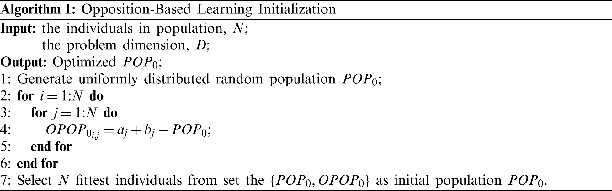
As mentioned above, OBL can accelerate the evolutionary process without any prior knowledge. This advantage makes up for the slow progress of the ACGDE algorithm in the early generations. Therefore, two main steps are distinguishable for the original ACGDE, including initialization and the different mutant operator in the first five percent generations. Like most algorithms utilizing OBL for optimization, initialization in this algorithm is divided into four steps:

3) The candidate’s fitness is measured, which is performed for all P and P⌣ individuals.

4) The first N individuals with the best fitness are selected as the first generation.

When the initialization provides better individuals that are closer to the Pareto frontier, we can iterate over them. Since ACGDE also implements nondominated the sorting genetic algorithm II (NSGAII) [32] in its multi-objective framework to select the next generation, the second step is the mutant operator of NSGAII, genetic algorithm (GA), replace the both mutant operators PCG and NCG in the first five percent generations. The experiment discussed in Section 4 will show that this replacement step is very effective in improving the convergence speed and finding the Pareto front.

Although we have optimized the parameters of the algorithm at the same time, the experiments in the later section show that the strengthened initialization is the part with the biggest improvement. Therefore, the optimization of initialization is the most important step for SIACGDE.

Here, the paper will focus on how the strengthened initialization and ACGDE mutant operator interact with each other. With better initial conditions, the cross-generation mutant operators, NCG and PCG, begin to play a stronger role than its predecessor in SIACGDE algorithm. The flow of SIACGDE is presented in Algorithm 2.

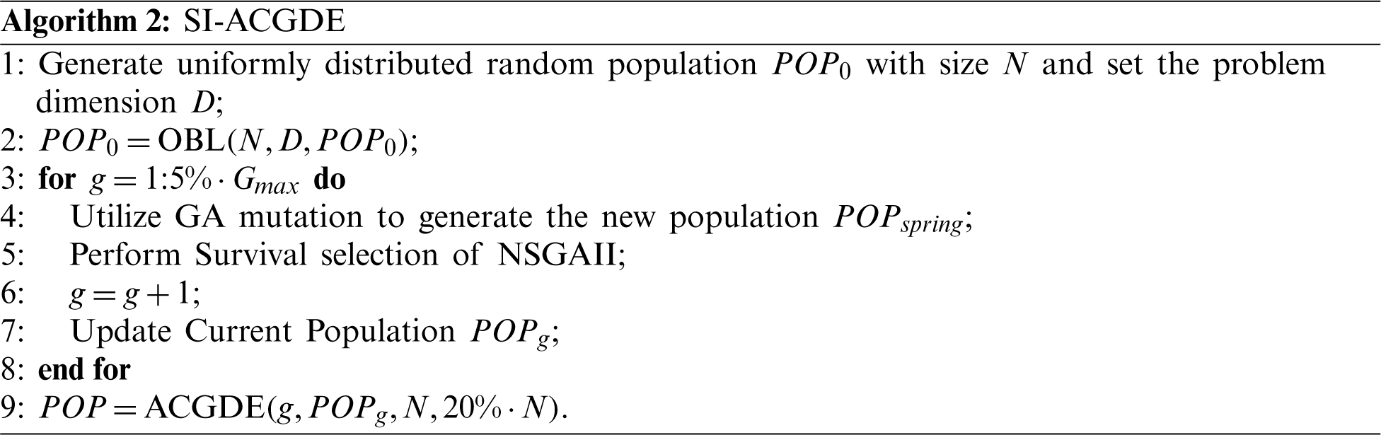
At the beginning, the individuals will be iterated rapidly in previous generations by NSGAII, and the obtained offspring can be used in SIACGDE. According to our experiment, it can be concluded that the iteration speed of NSGAII is obviously faster than the original algorithm in the initial stage. Furthermore, the addition of OBL makes the first few generations of individuals significantly better than the random initial individuals. In the process of evolution, GA mutates through two random parents, which does not depend on the individual differences between the two parents. This is actually an advantage in the early stage of evolution, compared with mutation NCG and PCG. If the previous operators are still used at early stage of evolution, the characteristics of these two operators will not play out. After several generations, the connection between populations is slowly established. At this time, this connection can not be used effectively by GA operator. Therefore, each generation is better than the previous generation, which can exactly match the cross-generation mechanism. This step is mainly for the two mutation NCG and PCG to obtain more obvious difference between generations.

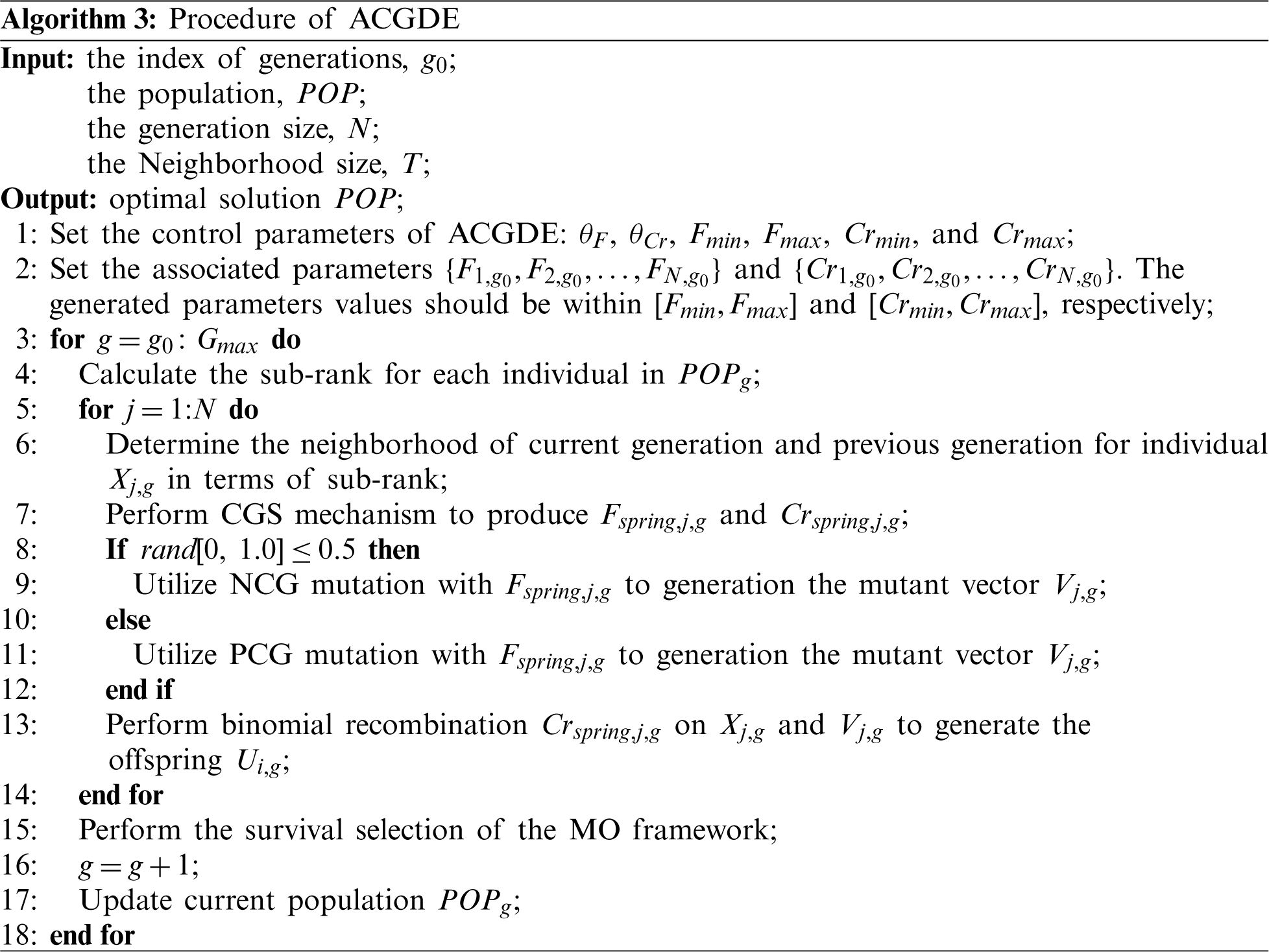
NCG is a mutation operator in which all mutated individuals are selected from the range of the Neighborhood. NCG has a narrower search range than PCG so that the individuals produced by NCG are more targeted and sensitive to generational differences. On the other hand, PCG has a wider search space, maintaining population diversity while avoiding a purely stochastic exploration. Both NCG and PCG mutations have a 50% chance of being used, which achieves a tradeoff between exploitation and exploration.

Then, the process is repeated until the termination condition is reached. Algorithm 3 shows the steps of the original ACGDE.

In this section, we discuss the performance of SIACGDE in the experiments. To fairly show performance comparisons, the same parameters are used in both algorithms, except for the change in the size of the Neighborhood. And the reason is described in the Subsection 3. Here, the experiment is presented in three subsections. First, the metrics used in this experiment are introduced in Subsection 1. Then, the comparison of seven common and state-of-the-art algorithms, including ACGDE, with the proposed SIACGDE algorithm on 24 frequently used MO benchmark problems (ZDT [40], DTLZ [41], VNT [42], and WFG [43]) is discussed in Subsection 2. The last subsection describes the tested effectiveness of the components of SIACGDE.

To date, there are a number of metrics to quantify the optimality of a solution set and the performance of multi-objective evolutionary algorithms (MOEAs) in multi-objective optimization (MOO). Each metric has its own set of performance criteria, which are divided into four categories: Capacity, Convergence, Diversity, and Convergence-Diversity. In this study, three metrics, including inverted generational distance (IGD) [35], Spread [36], Coverage over Pareto front (CPF) [37], and hypervolume (HV) [44], are selected to evaluate the performance of the algorithm in terms of direction diversity and convergence-diversity. Among them, IGD is the most common and effective metrics to evaluate the performance of the algorithm.

4.2 The Performance of Strengthened Initialization of Adaptive Cross-Generation Differential Evolution

To evaluate the competitiveness of the algorithm, we selected six state-of-the-art algorithms in addition to ACGDE for comparison. These include SIACGDE, ACGDE, and NSGAII, which were introduced earlier, and two common improved DE algorithms, GDE3 [26] and MOEADDE [45]. Other algorithms to be compared are LCSA [46], LMEA [47], and the improved version SPEA2SDE [48] of SPEA2 [49], which have been released in recent years. These seven algorithms were chosen for two reasons. First, some of algorithms, like MOEADDE, are variants that utilize the DE characteristics, and the effect of the comparison can more directly explain the validity of the proposed algorithm. Second, all improved algorithms are superior to their respective original algorithm in most problems. The experimental results of metrics are shown in Tables 1, 2 and Appendix A, respectively, where the best performance on each problem is bolded.

And the results were 30 independently run tests on each test problem for each MOEA algorithm. And the termination condition of eight algorithms is reaching maximum evolution of 10,000.

The values IGD of these seven algorithms for test functions can be shown in Table 1, from which it can be concluded that SIACGDE is the best algorithm on the most test functions. The relatively new algorithm LMEA follows as the second best. The convergence and diversity performance of the LMEA and LCSA algorithm are more excellent other algorithms except for SIACGDE which can be seen from the values of IGD. The reason why SIACGDE does not have a large advantage in some problems is mainly because the algorithm’s ability to deal with more complex Pareto frontier problems or problems with too many decision variables is not far beyond the sate-of-the-art algorithms. However, SIACGDE has achieved a good balance between search ability and convergence ability. Its main goal is to effectively infer the Pareto frontier position based on the information of two generations in multi-objective problems. Therefore, in most problems, SIACGDE have achieved best value of IGD in eight algorithms.

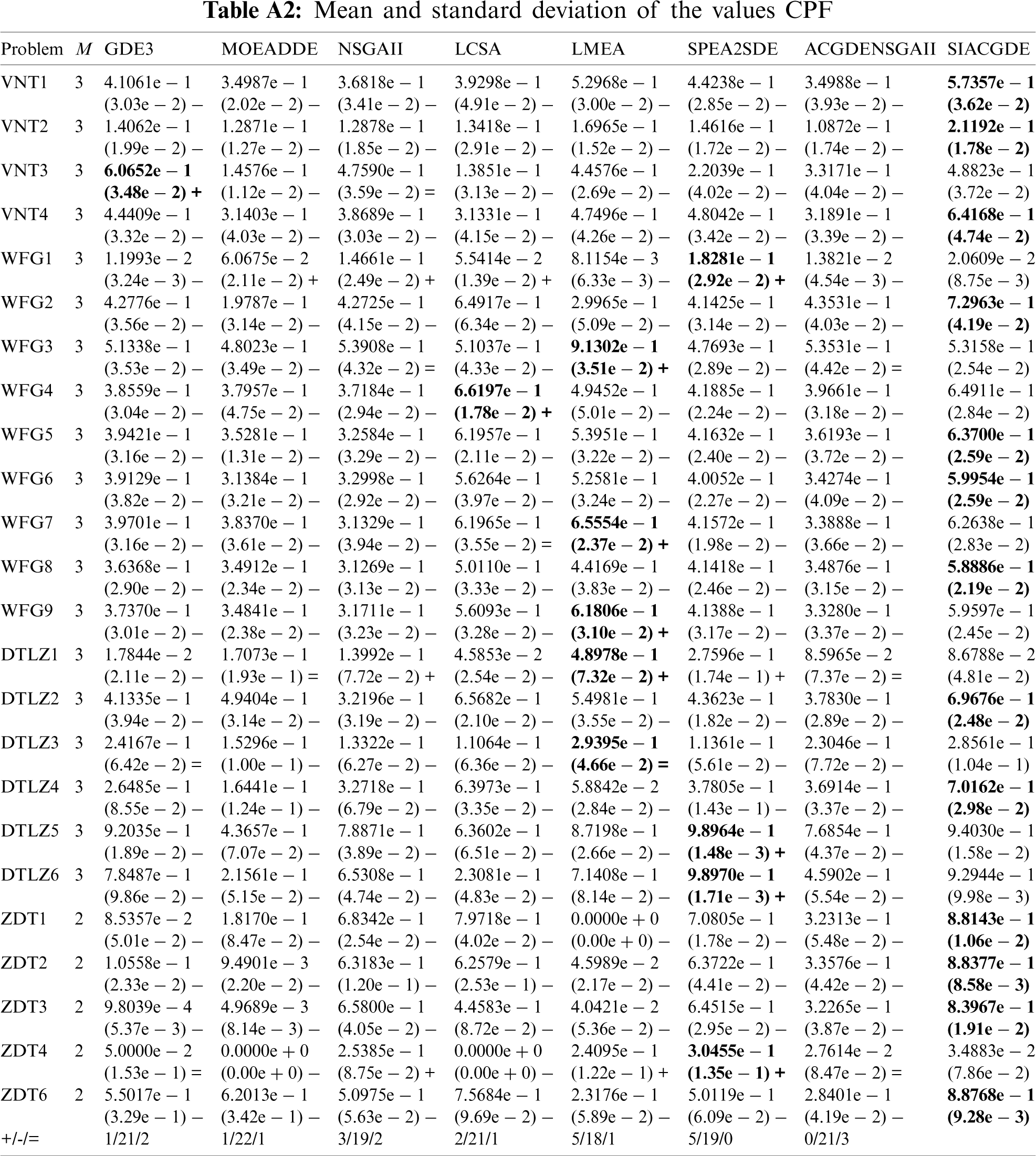
In order to show the performance of the algorithms in more angles, two metrics that are rarely considered in most experiments are also added in this experiment. As shown in Table A1 (the first table in Appendix A), the indicator Spread of SIACGDE performed best on 37 benchmarks, and SIACGDE has strong competitiveness on MOP. Finally, the experimental results from using the metric CPF in Table A2 (the second table in Appendix A) reveal that it is as dominant as the other two metrics in a total of 8 algorithms, also demonstrating strong performance of SIACGDE in coverage over the Pareto front.

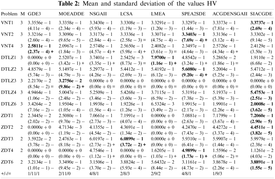
The bold font represents the best performance on this problem. Where the symbols ‘+’, ‘ −’ and ‘=’ indicate the results of compared algorithm is significantly better, significantly worse, and statistically similar to that obtained by SIACGDED at a 0.05 level by the Wilcoxon’s rank sum test, respectively.

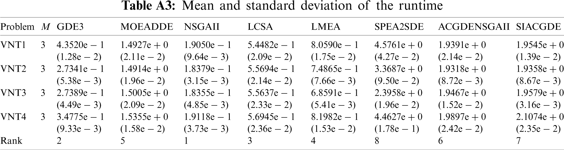
Among the metrics that show convergence-diversity performance, the most effective and popular is HV. And we showed the performance comparison of eight algorithms in Table A3 (the third table in Appendix A). As the same of previous results of three metrics, SIACGDE is the best performing one of the eight algorithms. Especially in a two-dimensional function which the real Pareto front is a curve, the effect of SIACGDE is the most obvious. Due to its cross-generation search mechanism, the problem ZDT1-2 is solved very well. And the cross-generation mechanism will illustrate its advantages in the next subsection. From multiple perspectives, it can be concluded that SIACGDE is an algorithm with excellent solving ability.

In addition, we compared the runtime of eight algorithms on VNT1∼4 [42] in Table 2. Among them, the shortest runtime is NSGAII. This shows that NSGAII as an excellent classic algorithm, it is relatively simple operators, which greatly saves calculation time. But at the same time, the performance of NSGAII is no longer competitive. The runtime of GDE3, LCSA, and LMEA are in same order of magnitude, and their speed are slower than NSGAII. This is because the algorithm has a certain improvement in searching or selection, which makes the algorithm has better performance and leads to a long running time. The time complexity of SPEA2SDE of selection mechanism is too high, resulting in that SPEA2SDE is the slowest algorithm among the eight algorithms. Although the runtime of SIACGDE and ACGDE are different, the gap is not big. It is due to the fact that the two algorithms use same mutant operators in the middle and late stages of evolution, but the performance of the algorithm has been greatly improved due to the enhancement of the initial stage by SIACGDE. These can explain that under the same computing resources, SIACGDE can get better the convergence and diversity of the population.

In this experiment, the original algorithm ACGDE is based on NSGAII framework to select offspring. By comparing ACGDE with SIACGDE, we can see that the new algorithm has been greatly improved in terms of both diversity and finding solutions due to the difference between successive generations generated in the initial stage. In the first few generations of the original algorithm, the use of cross-generation information to make mutations could not find an effective way forward. At this point, the original mutation operator can be replaced by genetic operator to make better use of excellent individuals for searching. At the same time, opposition-based learning is applied to provide more excellent individuals for genetic operator and, thus, differences between individuals when the algorithm produces cross-generational replacement.

In this subsection, we describe the experiments that were performed to verify the effectiveness of the cross-generation mutation proposed in SIACGDE. That is to say, we used the adjacent individuals of the parent and to select offspring. The validity of this strategy must be carried out under the premise that there is an obvious evolution in the two generations, so we suspended the experiment in the middle of evolution to observe. When SIACGDE ran the process of ZDT1 solution, we randomly selected two generations of experimental data. According to the results shown in Fig. 1, it is obvious that almost all individuals in the offspring are better than or equal to the parent individuals, and almost all vectors generated by the difference between them converge towards the Pareto front. Each generation moves forward, as described above, and eventually reaches the optimal solution.

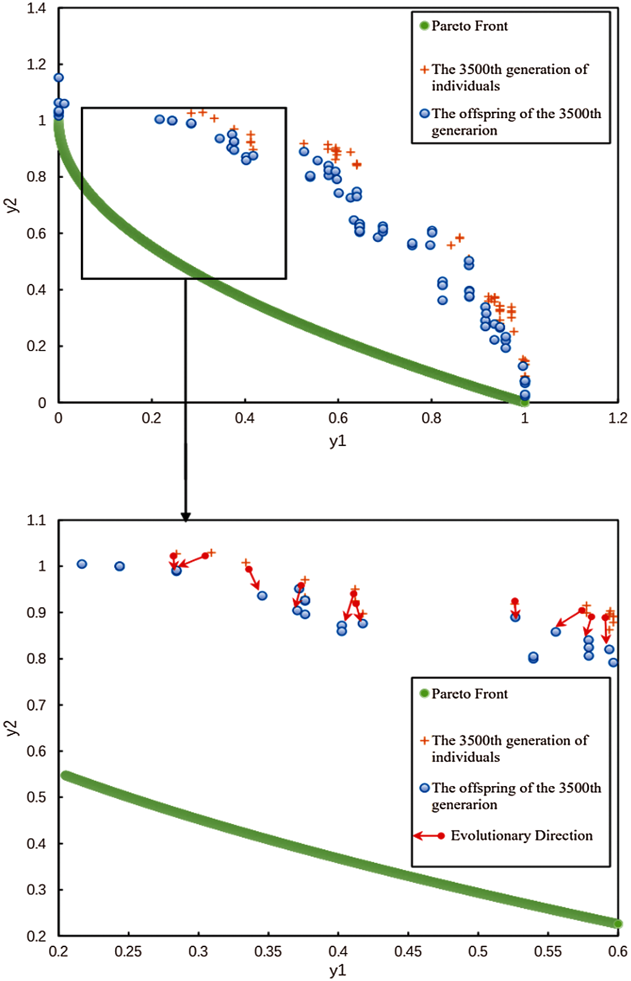
Figure 1: Procedure of SIACGDE and the relationship between parents and offspring individuals. The data include the 3500th generation of the algorithm running in ZDT1 and its next generation. The PF is the PF of ZDT1

From the above experiments, we can see that the NCG mutation factor plays a key role in finding the optimal solution, and the size of the Neighborhood is the most important parameter in NCG. Therefore, we must find the best value of Neighborhood size to achieve the optimal performance of the algorithm. In the experimental, this value is determined by changing the size of Neighborhood, where the size refers to the percentage of the population size, with the other parameters remained unchanged. We can see from Fig. 2 that the optimal value of Neighborhood size in the three test functions, DTLZ1, DTLZ2, and DTLZ3, is 20%. Starting from a value of 20%, as the size becomes smaller, the IGD becomes larger and unstable, which means that the convergence and diversity of population are getting worse and worse. As the value of size increases towards 30%, greater error is observed. Therefore, the proportion of Neighborhood size is fixed at 20% and implemented into SIACGDE.

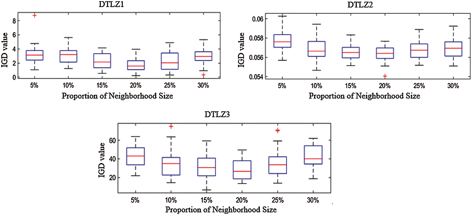
Figure 2: Boxplots of the IGD values over 30 independent runs. The simulations were performed on DTLZ1-DTLZ3 separately

In the last subsection of the experiment, we tested the GA factor that has the greatest impact on the original ACGDE algorithm, the GA replaces the initial stage of mutation. The purpose of this experiment is to find how many generations in initial stage of GA will maximize the algorithm convergence of performance. Before the experiment, for the convenience of comparison, we named different GA proportions of SIACGDE: When the SIACGDE just used OBL in initialization, this model is SIACGDEI. When the proportion of GA in whole algorithm is 10%, this model is SIACGDEII. When the proportion of GA in whole algorithm is 15%, this model is SIACGDEIII. The SIACGDE algorithm, used in this paper, the proportion of GA in whole algorithm is 5%.

Fig. 3 illustrates the performance of the SIACGDE algorithms and the original ACGDE algorithm on ZDT1-ZDT3. It can be seen that in the three tests, only the first 5%N generation using GA achieved the best convergence. Therefore, it can be deduced that the convergence of the algorithm is affected by the proportion of GA.

Figure 3: IGD values of four SIACGDE algorithms and ACGDE algorithm on ZDT1-ZDT2 (a) IGD of ZDT1 (b) IGD of ZDT2 (c) IGD of ZDT3 (d) Legend

This paper describes the improvement of the ACGDE algorithm by introducing the GA mutant operator in the initial stage, which corrects for the lack of search ability. SIACGDE specifically developed a new initialization method for two cross-generation mutations, NCG and PCG, so that the new alternative individuals are more suitable for the two mutations. Furthermore, the OBL mechanism is added to improve the efficiency of evolution. Experimental results demonstrate the significant improvements of two adjusted versions of ACGDE and that SIACGDE is obviously superior to the other six state-of-the-art algorithms. However, our proposed algorithm has its limitations. Firstly, when the real Pareto front is not continuous, the solving ability is reduced, which is also caused by the characteristics of cross-generation mutation. Secondly, the algorithm has no ability to deal with the problem of constraints.

In the future, the first plan is to find a method to deal with constraints matching the algorithm, so as to solve the real-world problems [50,51] and make SIACGDE more vitality. Then we plan to adopt a dynamic adaptive mechanism for the ratio of several mutant operators used in SIACGDE. We will also aim to develop a better strategy to apply in the early stage of the algorithm so that it could be implemented into other many-objective frameworks to deal with higher dimensional problems. In addition, introducing more generations to participate in evolution will be considered. Finally, we will try to apply the concept of cross-generation evolution to other metaheuristic algorithms to examine its universe use.

Acknowledgement: The authors thank the Ocean University of China for their support in this work.

Conflicts of Interest: The authors declare that they have no conflicts of interest to report regarding the present study.

References

Storn, R. (1995). Differrential evolution-a simple and efficient adaptive scheme for global optimization over continuous spaces. Technical Report, 952.
Guo, S., & Yang, C. (2014). Enhancing differential evolution utilizing eigenvector-based crossover operator. IEEE Transactions on Evolutionary Computation, 19(1), 31-49. [Google Scholar] [CrossRef]
Meng, Z., Chen, Y., Li, X., & Lin, F. (2020). PaDE-NPC: Parameter adaptive differential evolution with novel parameter control for single-objective optimization. IEEE Access, 8, 139460-139478. [Google Scholar] [CrossRef]
Ozer, A. B. (2010). CIDE: Chaotically initialized differential evolution. Expert Systems with Applications, 37(6), 4632-4641. [Google Scholar] [CrossRef]
Li, G., Wang, G. G., & Wang, S. (2021). Two-population coevolutionary algorithm with dynamic learning strategy for many-objective optimization. Mathematics, 9(4), 420. [Google Scholar] [CrossRef]
Zhang, H., Wang, G. G., Dong, J., & Gandomi, A. H. (2021). Improved NSGA-III with second-order difference random strategy for dynamic multi-objective optimization. Processes, 9(6), 911. [Google Scholar] [CrossRef]
Yi, J. H., Xing, L. N., Wang, G. G., Dong, J., & Vasilakos, A. V. (2020). Behavior of crossover operators in NSGA-III for large-scale optimization problems. Information Sciences, 509(15), 470-487. [Google Scholar] [CrossRef]
Zhang, Y., Wang, G. G., Li, K., Yeh, W. C., & Jian, M. (2020). Enhancing MOEA/D with information feedback models for large-scale many-objective optimization. Information Sciences, 522(1), 1-16. [Google Scholar] [CrossRef]
Gong, W., & Cai, Z. (2013). Differential evolution with ranking-based mutation operators. IEEE Transactions on Cybernetics, 43(6), 2066-2081. [Google Scholar] [CrossRef]
Tang, L., Dong, Y., & Liu, J. (2014). Differential evolution with an individual-dependent mechanism. IEEE Transactions on Evolutionary Computation, 19(4), 560-574. [Google Scholar] [CrossRef]
Gao, D., & Wang, G. G. (2020). Solving fuzzy job-shop scheduling problem using DE algorithm improved by a selection mechanism. IEEE Transactions on Fuzzy Systems, 28(12), 3265-3275. [Google Scholar] [CrossRef]
Wang, G. G., Cai, X., Cui, Z., Min, G., & Chen, J. (2020). High performance computing for cyber physical social systems by using evolutionary multi-objective optimization algorithm. IEEE Transactions on Emerging Topics in Computing, 8(1), 20-30. [Google Scholar] [CrossRef]
Huang, Y., Li, W., Tian, F., & Meng, X. (2020). A fitness landscape ruggedness multiobjective differential evolution algorithm with a reinforcement learning strategy. Applied Soft Computing, 96(1), 106693. [Google Scholar] [CrossRef]
Carvalho, J. P. G., Carvalho, É. C., Vargas, D. E., Hallak, P. H., & Lima, B. S. (2021). Multi-objective optimum design of truss structures using differential evolution algorithms. Computers Structures, 252(10), 106544. [Google Scholar] [CrossRef]
Cheng, J., Yen, G. G., & Zhang, G. (2016). A grid-based adaptive multi-objective differential evolution algorithm. Information Sciences, 367(1), 890-908. [Google Scholar] [CrossRef]
Zhang, Y., Gong, D., Gao, X., Tian, T., & Sun, X. (2020). Binary differential evolution with self-learning for multi-objective feature selection. Information Sciences, 507(2), 67-85. [Google Scholar] [CrossRef]
Pan, Z., Fang, S., & Wang, H. (2020). LightGBM technique and differential evolution algorithm-based multi-objective optimization design of DS-APMM. IEEE Transactions on Energy Conversion, 10(1), 1109. [Google Scholar] [CrossRef]
Deng, W., Liu, H., Xu, J., Zhao, H., & Song, Y. (2020). An improved quantum-inspired differential evolution algorithm for deep belief network. IEEE Transactions on Instrumentation Measurement, 69(10), 7319-7327. [Google Scholar] [CrossRef]
Mininno, E., Neri, F., Cupertino, F., & Naso, D. (2010). Compact differential evolution. IEEE Transactions on Evolutionary Computation, 15(1), 32-54. [Google Scholar] [CrossRef]
Liu, Y., Chen, Y., & Yang, G. (2018). Developing multiobjective equilibrium optimization method for sustainable uncertain supply chain planning problems. IEEE Transactions on Fuzzy Systems, 27(5), 1037-1051. [Google Scholar] [CrossRef]
Wang, Y., Liu, Z. Z., Li, J., Li, H. X., & Wang, J. (2018). On the selection of solutions for mutation in differential evolution. Frontiers of Computer Science, 12(2), 297-315. [Google Scholar] [CrossRef]
Sun, G., Xu, G., & Jiang, N. (2020). A simple differential evolution with time-varying strategy for continuous optimization. Soft Computing, 24(4), 2727-2747. [Google Scholar] [CrossRef]
Cardenas-Montes, M. (2018). Weibull-based scaled-differences schema for differential evolution. Swarm Evolutionary Computation, 38(4), 79-93. [Google Scholar] [CrossRef]
Mesejo, P., Ugolotti, R., Cunto, F. D., Giacobini, M., & Cagnoni, S. (2013). Automatic hippocampus localization in histological images using differential evolution-based deformable models. Pattern Recognition Letters, 34(3), 299-307. [Google Scholar] [CrossRef]
Awad, N. H., Ali, M. Z., Suganthan, P. N., & Reynolds, R. G. (2017). CADE: A hybridization of cultural algorithm and differential evolution for numerical optimization. Information Sciences, 378(6), 215-241. [Google Scholar] [CrossRef]
Kukkonen, S., & Lampinen, J. (2005). GDE3: The third evolution step of generalized differential evolution. 2005 IEEE Congress on Evolutionary Computation, 3, 443-450. [Google Scholar]
Das, S., Abraham, A., Chakraborty, U. K., & Konar, A. (2009). Differential evolution using a neighborhood-based mutation operator. IEEE Transactions on Evolutionary Computation, 13(3), 526-553. [Google Scholar] [CrossRef]
Wang, Y., Cai, Z., & Zhang, Q. (2011). Differential evolution with composite trial vector generation strategies and control parameters. IEEE Transactions on Evolutionary Computation, 15(1), 55-66. [Google Scholar] [CrossRef]
Storn, R. (1996). On the usage of differential evolution for function optimization. Proceedings of North American Fuzzy Information Processing, pp. 519–523. Berkeley, USA.
Pant, M., Zaheer, H., Garcia-Hernandez, L., & Abraham, A. (2020). Differential evolution: A review of more than two decades of research. Engineering Applications of Artificial Intelligence, 90(1), 103479. [Google Scholar] [CrossRef]
Qiu, X., Xu, J., Tan, K., & Abbass, H. A. (2015). Adaptive cross-generation differential evolution operators for multiobjective optimization. IEEE Transactions on Evolutionary Computation, 20(2), 232-244. [Google Scholar] [CrossRef]
Deb, K., Agrawal, S., Pratap, A., Meyarivan, T. (2000). A fast elitist non-dominated sorting genetic algorithm for multi-objective optimization: NSGA-II. International Conference on Parallel Problem Solving from Nature, pp. 849–858. Springer, Berlin, Heidelberg.
Tizhoosh, H. R. (2005). Opposition-based learning: A new scheme for machine intelligence. International Conference on Computational Intelligence for Modelling, Control and Automation and International Conference on Intelligent Agents, Web Technologies and Internet Commerce, pp. 695–701. Vienna, Austria.
Rahnamayan, S., Tizhoosh, H. R., & Salama, M. M. (2008). Opposition-based differential evolution. IEEE Transactions on Evolutionary Computation, 12(1), 64-79. [Google Scholar] [CrossRef]
Jiang, S., Ong, Y. S., Zhang, J., & Feng, L. (2014). Consistencies and contradictions of performance metrics in multiobjective optimization. IEEE Transactions on Cybernetics, 44(12), 2391-2404. [Google Scholar] [CrossRef]
Wang, Y., Wu, L., & Yuan, X. (2010). Multi-objective self-adaptive differential evolution with elitist archive and crowding entropy-based diversity measure. Soft Computing, 14(3), 193-209. [Google Scholar] [CrossRef]
Tian, Y., Cheng, R., Zhang, X., Li, M., & Jin, Y. (2019). Diversity assessment of multi-objective evolutionary algorithms: Performance metric and benchmark problems [Research Frontier]. IEEE Computational Intelligence Magazine, 14(3), 61-74. [Google Scholar] [CrossRef]
Robič, T., Filipič, B. (2005). Differential evolution for multiobjective optimization. International Conference on Evolutionary Multi-Criterion Optimization, pp. 520–533. Springer, Berlin, Heidelberg.
Mahdavi, S., Rahnamayan, S., & Deb, K. (2018). Opposition based learning: A literature review. Swarm Evolutionary Computation, 39(8), 1-23. [Google Scholar] [CrossRef]
Zitzler, E., Deb, K., & Thiele, L. (2000). Comparison of multiobjective evolutionary algorithms: Empirical results. Evolutionary Computation, 8(2), 173-195. [Google Scholar] [CrossRef]
Jain, H., & Deb, K. (2013). An evolutionary many-objective optimization algorithm using reference-point based nondominated sorting approach, part II: Handling constraints and extending to an adaptive approach. IEEE Transactions on Evolutionary Computation, 18(4), 602-622. [Google Scholar] [CrossRef]
Vlennet, R., Fonteix, C., & Marc, I. (1996). Multicriteria optimization using a genetic algorithm for determining a Pareto set. International Journal of Systems Science, 27(2), 255-260. [Google Scholar] [CrossRef]
Huband, S., Hingston, P., Barone, L., & While, L. (2006). A review of multiobjective test problems and a scalable test problem toolkit. IEEE Transactions on Evolutionary Computation, 10(5), 477-506. [Google Scholar] [CrossRef]
Zitzler, E., & Thiele, L. (1999). Multiobjective evolutionary algorithms: A comparative case study and the strength Pareto approach. IEEE Transactions on Evolutionary Computation, 3(4), 257-271. [Google Scholar] [CrossRef]
Li, H., & Zhang, Q. (2008). Multiobjective optimization problems with complicated Pareto sets, MOEA/D and NSGA-II. IEEE Transactions on Evolutionary Computation, 13(2), 284-302. [Google Scholar] [CrossRef]
Zille, H. (2019). Large-scale multi-objective optimisation: New approaches and a classification of the state-of-the-art (PhD Dissertation). Germany: Otto-vonGuericke-Universitaet Magdeburg
Zhang, X., Tian, Y., Cheng, R., & Jin, Y. (2016). A decision variable clustering-based evolutionary algorithm for large-scale many-objective optimization. IEEE Transactions on Evolutionary Computation, 22(1), 97-112. [Google Scholar] [CrossRef]
Li, M., Yang, S., & Liu, X. (2013). Shift-based density estimation for Pareto-based algorithms in many-objective optimization. IEEE Transactions on Evolutionary Computation, 18(3), 348-365. [Google Scholar] [CrossRef]
Zitzler, E., Laumanns, M., Thiele, L. (2001). SPEA2: Improving the strength Pareto evolutionary algorithm. TIK-Report, 103.
Kumar, A., Wu, G., Ali, M. Z., Mallipeddi, R., & Suganthan, P. N. (2020). A test-suite of non-convex constrained optimization problems from the real-world and some baseline results. Swarm Evolutionary Computation, 56, 100693. [Google Scholar] [CrossRef]
Chamorro, H. R., Riano, I., Gerndt, R., Zelinka, I., & Gonzalez-sLongatt, F. (2019). Synthetic inertia control based on fuzzy adaptive differential evolution. International Journal of Electrical Power Energy Systems, 105(1), 803-813. [Google Scholar] [CrossRef]