| Computer Modeling in Engineering & Sciences |
DOI: 10.32604/cmes.2022.019199
ARTICLE
New Hybrid EWMA Charts for Efficient Process Dispersion Monitoring with Application in Automobile Industry
1Faculty of Economics, Taiyuan Normal University, Taiyuan, 030619, China
2Department of Mathematics and Statistics, Riphah International University, Islamabad, 44000, Pakistan
3Department of Mathematics, Women University of Azad Jammu and Kashmir, Bagh, 12500, Pakistan
4Department of Statistics, University of Azad Jammu and Kashmir, Muzaffarabad, 13100, Pakistan
5School of Statistics, Shanxi University of Finance and Economics, Taiyuan, 030619, China
*Corresponding Author: Syed Masroor Anwar. Email: masroorstatistics@gmail.com
Received: 08 September 2021; Accepted: 09 November 2021
Abstract: The EWMA charts are the well-known memory-type charts used for monitoring the small-to-intermediate shifts in the process parameters (location and/or dispersion). The hybrid EWMA (HEWMA) charts are enhanced version of the EWMA charts, which effectively monitor the process parameters. This paper aims to develop two new upper-sided HEWMA charts for monitoring shifts in process variance, i.e., HEWMA1 and HEWMA2 charts. The design structures of the proposed HEWMA1 and HEWMA2 charts are based on the concept of integrating the features of two EWMA charts. The HEWMA1 and HEWMA2 charts plotting statistics are developed using one EWMA statistic as input for the other EWMA statistic. A Monte Carlo simulations method is used as a computational technique to determine the numerical results for the performance characteristics, such as average run length (ARL), median run length, and standard deviation run length (SDRL) for assessing the performance of the proposed HEWMA1 and HEWMA2 charts. In addition, to evaluate the overall performance of the proposed HEWMA1 and HEWMA2 charts, other numerical measures consisting of the extra quadratic loss (EQL), relative average run length (RARL), and performance comparison index (PCI) are also computed. The proposed HEWMA1 and HEWMA2 charts are compared to some existing charts, such as CH, CEWMA, HEWMA, AEWMA HHW1, HHW2, AIB-EWMA-I, and AIB-EWMA-II charts, on the basis aforementioned numerical measures. The comparison reveals that the proposed HEWMA1 and HEWMA2 charts achieve better detection ability against the existing charts. In the end, a real-life data application is also provided to enhance the implementation of the proposed HEWMA1 and HEWMA2 charts practically.
Keywords: Average run length; extra quadratic loss; memory-type charts; Monte Carlo simulations; smoothing parameter
Control charts are the essential tools of the statistical process monitoring (SPM) toolkit, used to detect the shifts in manufacturing and production processes parameter(s). The control charts are generally classified into memory-type and memoryless-type charts [1]. The memoryless-type charts are used only for current information of the process, while the memory-type charts are based on both current and previous information of the process. The basic memoryless-type charts are the Shewhart charts, like the Shewhart
Roberts [3] was the first to introduce the classical EWMA chart for monitoring the mean level of the process. Later, Hunter et al. [4–7] further investigated the various EWMA-type charts in order to facilitate the application of the classical EWMA chart in mean process monitoring. Recent studies have shown that EWMA-type charts are the most useful tools for researchers. For example, Haq [8], Abbas et al. [9], Ali et al. [10], Tang et al. [11], Haq [12], Rasheed et al. [13], Rasheed et al. [14], etc., are the few recent references in this regard.
In general, most manufacturing and production processes have a shift in the mean level; however, the process variance (or standard deviation) may be shifted from the target in many practical situations. Domangue et al. [15] suggested that monitoring an increase in process variance is more important for the processes. Although the EWMA-types charts are primarily used in mean process monitoring; however, few works address the variance monitoring via these charts. For example, Crowder et al. [16] used the logarithmic transformation to the sample variance
The use of hybrid charts enhances the efficiency of traditional charts. For example, Haq [8] and Haq [28] proposed the HEWMA chart to monitor the mean level of the process. Later on, numerous authors used the HEWMA charts in different process monitoring schemes. The HEWMA charts are more efficient than the classical EWMA and CUSUM charts in terms of small to moderate shifts monitoring. For example, Aslam et al. [29] introduced the HEWMA chart to monitor the mean level of the process under repetitive sampling. Similarly, Aslam et al. [30] monitored the COM-Poisson process by designing the HEWMA chart. Equally, Aslam et al. [31] developed the mixed chart, named the HEWMA-CUSUM chart, for the Weibull process monitoring. Correspondingly, Noor-ul-Amin et al. [32] recommended the HEWMA chart for Phase-II mean monitoring, based on the auxiliary information. Besides, Aslam et al. [33] suggested the HEWMA-p chart to monitor the variance of the non-normal process. Also, Noor et al. [34] constructed the Bayesian HEWMA chart, using two loss functions, to monitor the mean level of the normal process. The other studies about the
The majority of manufacturing and service processes are affected by the gradual increase in process variance. The increase in the process variance indicates a deterioration in the process performance. This study's first and most important goal is to propose efficient charts with effective shifts detection ability in monitoring an increase in the process variances. So, motivated by Crowder et al. [16], Castagliola [19], and Haq [8], this study proposes two new HEWMA charts to monitor the increasing shifts in the process variance. The proposed charts are known as HEWMA1 and HEWMA2 charts. The design structure of the HEWMA1 chart uses the CH statistic as the input for the HEWMA1 statistic. In the same lines, the CEWMA statistic is considered an input to the HEWMA2 statistic to formulate the HEWMA2 chart. The Monte Carlo simulations are employed to compute the numerical results associated with average run length (
The remainder of the article is set out in the following way: Section 2 presents the existing methods. Likewise, Section 3 lays out the methodologies and formulation of the proposed HEWMA1 and HEWMA2 charts. In addition, the performance evaluation measures and simulation study are included in Section 4. Furthermore, Section 5 consists of the comparison and performance analysis of the proposed HEWMA1 and HEWMA2 charts against some existing charts. Section 6 offers a real-life data application to enhance the performance of the proposed HEWMA1 and HEWMA2 charts. The last section addresses the concluding remarks.
This section defines the process variable in Subsection 2.1. Similarly, Subsection 2.2 explains the details about the transformations to the sample variance. In addition, Subsections 2.3 to 2.6 provide the design and formulation of the CH, CEWMA, HHW2, and HEWMA charts for monitoring process variance, respectively.
Assuming, at the time
In order to implement the EWMA-type charts, the assumption of normality is required for the plotting statistic of the charts. However, because the sample variance
Let
where the ratio
Castagliola [19] recommended the three-parameter logarithmic transformation of
where
In order to detect the shifts in the process variance, Quesenberry [38] suggested another transformation defined as
where
Crowder et al. [16] introduced the CH chart, which monitored the process variance shifts. Let
where
.
In the case of large
The initial value of and
where
Castagliola [19] proposed the EWMA chart (also known as
The initial value of
The
where
Huwang et al. [18] proposed the EWMA chart to monitor the process variance, denoted as the HHW2 chart. Let
The initial value of and
In case of large
The
Ali et al. [23] followed the idea of [8] and designed the HEWMA chart for process variance. Let the IID
where
The control limit
When
where
Haq [8] suggested the HEWMA chart to monitor the process mean. Similarly, Ali et al. [23] presented the HEWMA chart's design structure for tracking the process variance. Following Haq [8], the HEWMA1 and HEWMA2 charts can be developed using Transformations I and II, respectively. These charts detect increasing shifts in process variance. The methodologies and construction of the HEWMA1 and HEWMA2 charts are, respectively, presented in Subsections 3.1 and 3.2.
The design structure for the HEWMA1 chart can be constructed using the CH statistic as input for the HEWMA1 statistic. Let defined the sequence of IID random variable, say
where
In order to monitor the increasing shift in the process, the HEWMA1 statistic is defined as
The initial value of
where
The initial value of
The lower-sided HEWMA1 chart detects OOC signals whenever
The two-sided HEWMA1 chart detects OOC signals whenever
In order to formulate the design of the HEWMA2 chart, the charting statistic of the CEWMA chart can be used as an input for the HEWMA2 statistic. Let
where
The HEWMA2 control limits
The control limits defined in Eq. (26) are known as the two-sided time-dependent control limits; however, in the case of large
In this case, The HEWMA2 chart triggers OOC signals whenever
The
4 Performance Analysis and Simulation Study
This section defines the performance evaluation measures, such as average run length in Subsection 4.1 and overall performance measures in Subsection 4.2. Similarly, the simulation study for the proposed HEWMA1 and HEWMA2 charts is designed in Subsection 4.3. Likewise, Subsection 4.4 provides the choices design parameters for the proposed HEWMA1 and HEWMA2 charts.
The most popular and commonly used performance evaluation measures are the
4.2 Overall Performance Evaluation Measures
The
The
where
4.2.2 Relative Average Run Length
Like the
where
4.2.3 Performance Comparison Index
The
The PCI value for the benchmark chart is equal to be 1, and for the rest of the charts,
The random sample of size
i) Specify sample size
ii) Generate random observations
iii) Compute the statistics,
iv) Using
v) Using
vi) Selected
vii) Plot the statistic
viii) Repeat Steps (ii)–(vii)
ix) For
4.4 Choices of Design Parameters
The design parameters for the proposed HEWMA1 and HEWMA2 charts are the smoothing constants
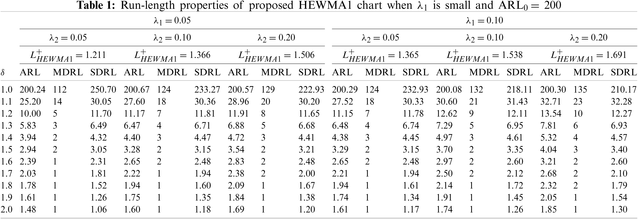
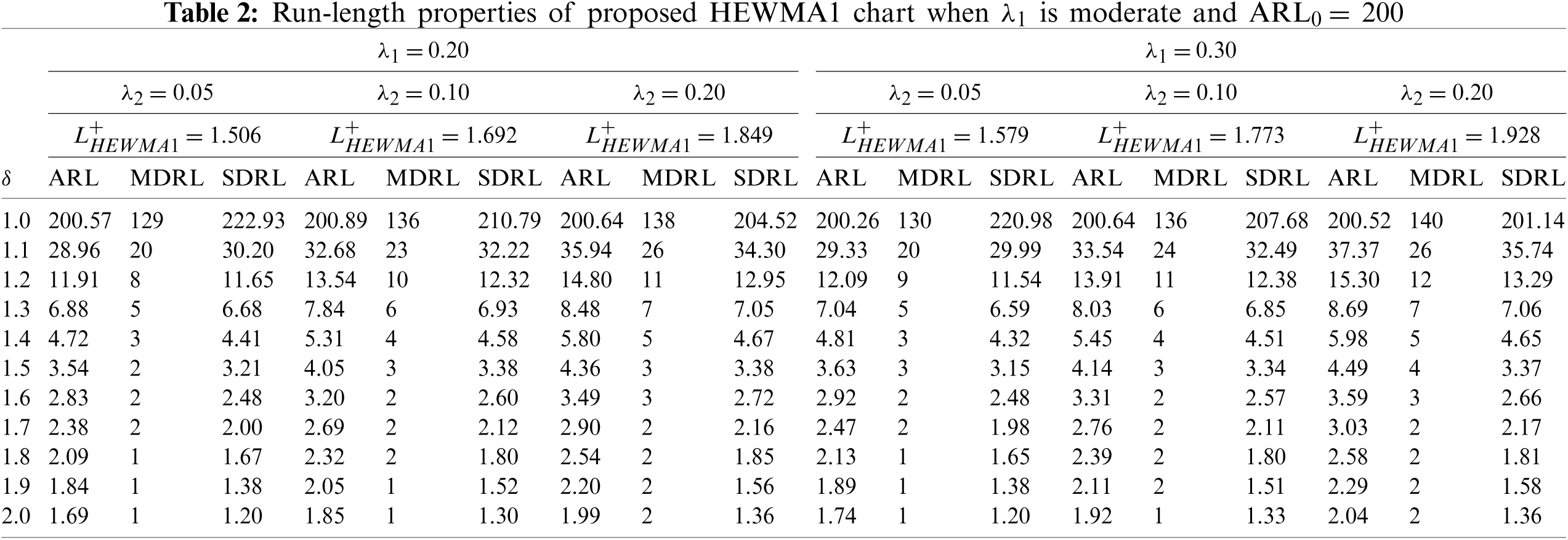

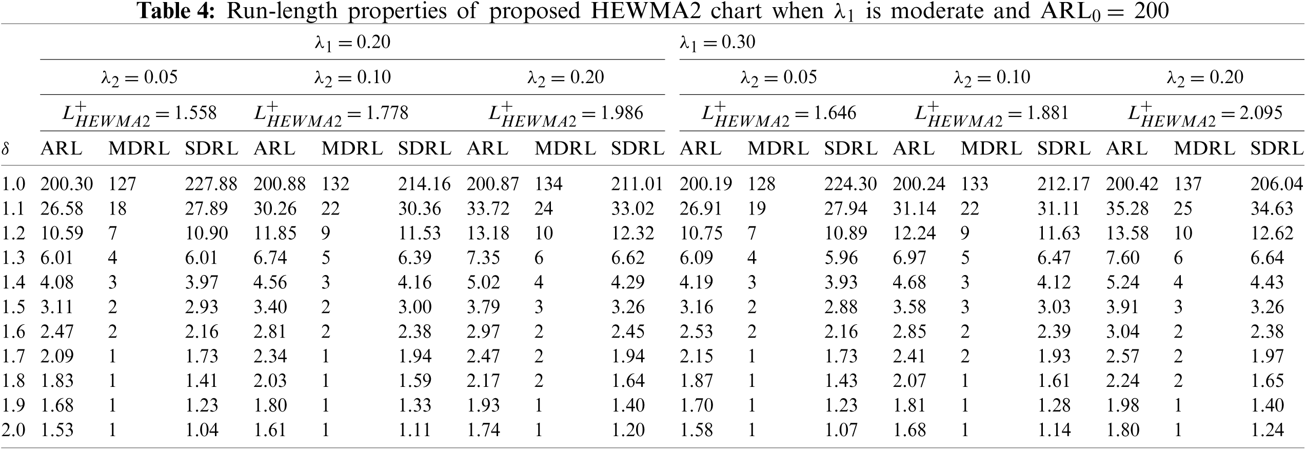
This section addresses the detailed comparative study of the proposed charts to the existing charts. The ARL values in Tables 1–4 reveal that the HEWMA2 chart outperforms the HEWMA1 chart; therefore, the HEWMA2 chart is recommended to compare with the existing charts for better detection performance. Thus the HEWMA2 charts is compared against the existing CH [16], CEWMA [19], HEWMA [23], AEWMA [45], AIBEWMA1, and AIBEWMA2 [22] charts. Table 5 presents the ARL values for comparison, while Table 6 contains the overall performance values. The following Subsections offer further details about the comparisons.
The proposed HEWMA2 chart achieves better performance against the CH chart. For example, at
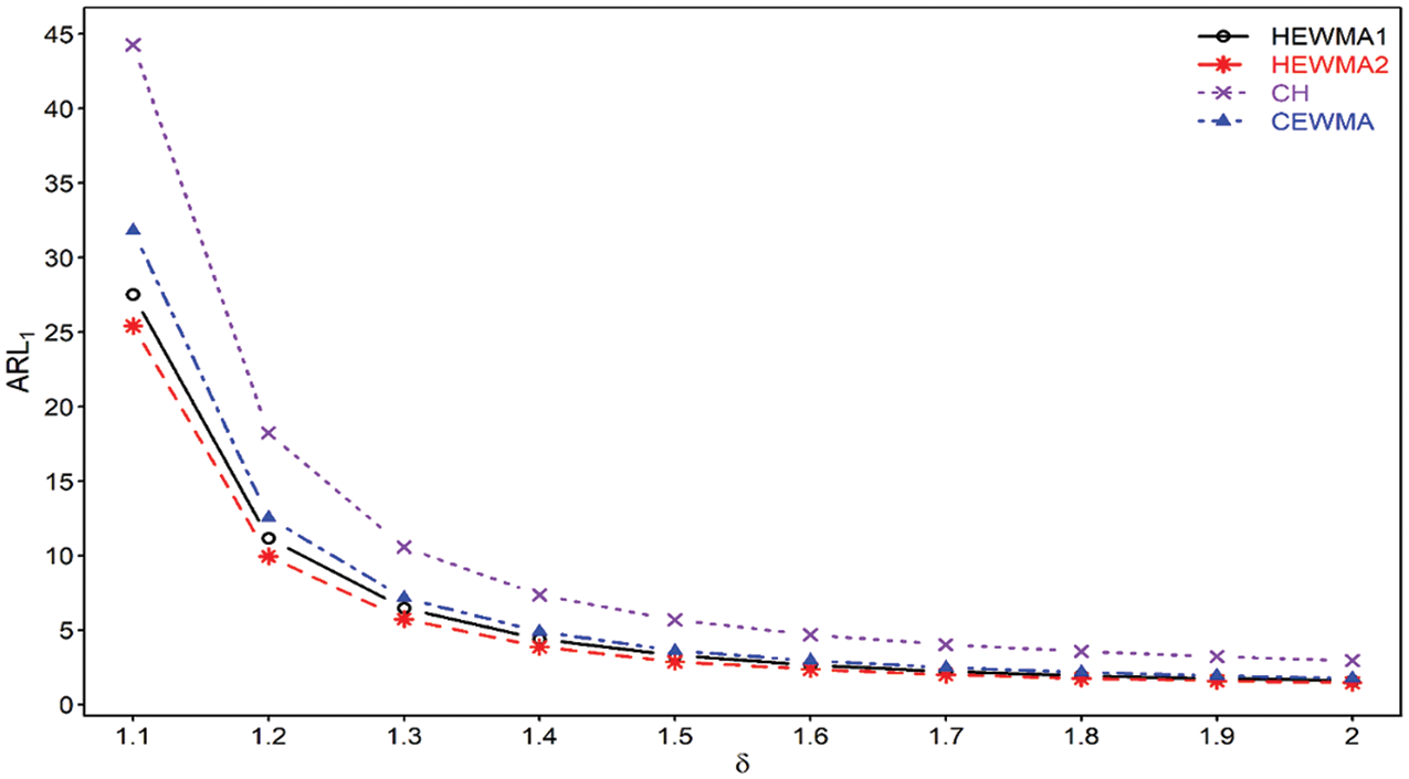
Figure 1: Comparison of proposed HEWMA1 and HEWMA2 charts with CH and CEWMA charts at
The proposed HEWMA2 chart shows lower
The proposed HEWMA2 chart achieves superior performance over the HEWMA chart. For instance, at
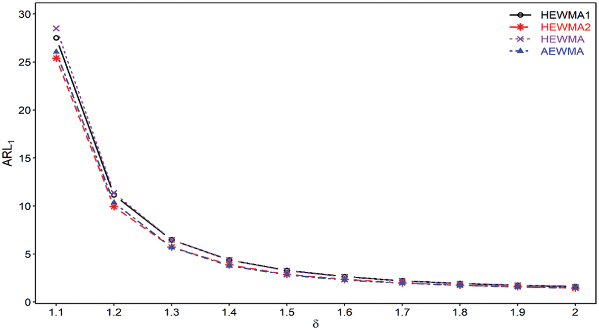
Figure 2: Comparison of proposed HEWMA1 and HEWMA2 charts with HEWMA and AEWMA charts at
Haq [45] developed the adaptive EWMA (AEWMA) chart for monitoring the process variance. The proposed HEWMA2 chart is compared to the AEWMA chart at
5.5 Proposed vs. AIBEWMA1 and AIBEWMA2 Charts
Haq [22] proposed the AIBEWMA1 and AIBEWMA2 charts for monitoring the process variance. The comparison of the HEWMA2 chart against the AIBEWMA1 and AIBEWMA2 charts demonstrates that the proposed HEWMA2 chart is more efficient than the AIBEWMA1 and AIBEWMA2 charts. For example, with chart properties, i.e.,
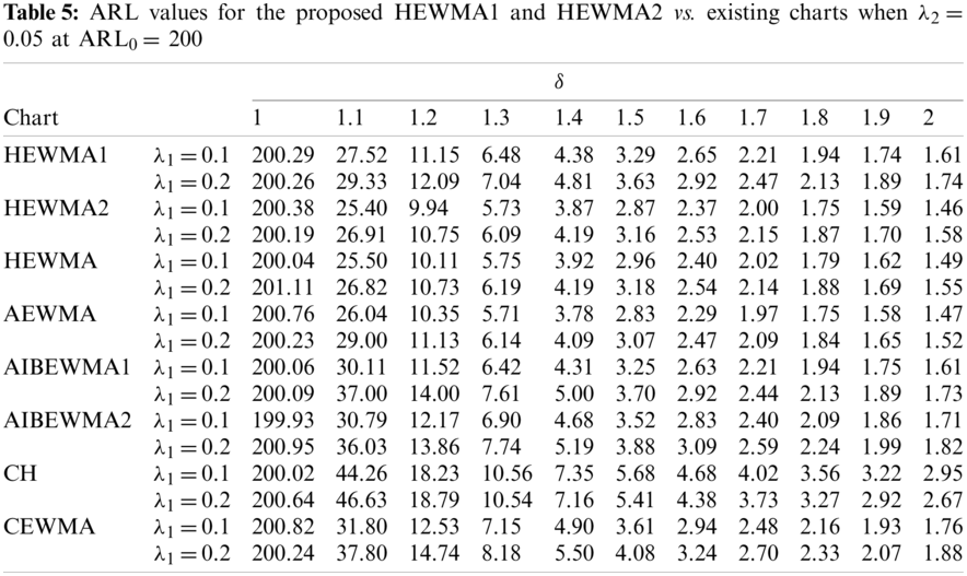
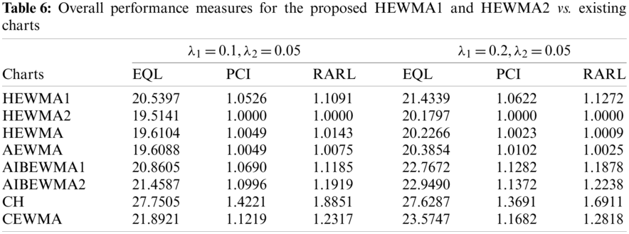
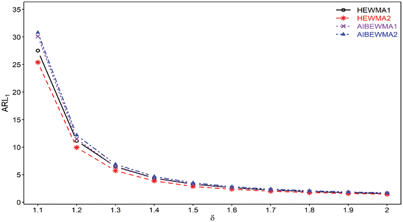
Figure 3: Comparison of proposed HEWMA1 and HEWMA2 charts with AIBEWMA1 and AIBEWMA2 charts at
6 Important Points of the Study
A few important points related to the HEWMA1 and HEWMA2 charts can be listed as:
i) The HEWMA statistics undoubtedly boost the efficiency of the proposed HEWMA1 and HEWMA2 charts.
ii) The proposed HEWMA2 chart has better detection performance than the proposed HEWMA1 chart (see Tables 1–4).
iii) At different parametric settings, the
iv) The overall performance reveals the dominance of HEWMA1 and HEWMA2 charts over the CH, CEWMA, HEWMA, AEWMA, AIBEWMA1, and AIBEWMA2 charts (see Section 5).
v) The proposed HEWMA1 and HEWMA2 charts have better
vi) The control limit coefficient
7 Real-life Application of the Proposed Charts
This subsection explains the application of the proposed HEWMA1 and HEWMA2 charts to real-life data. For this purpose, the real-life data are considered, representing the inside diameter of the cylinder bores in an engine block. These real-life data are used by [46,47] in their studies. The data comprise 30 samples, each size
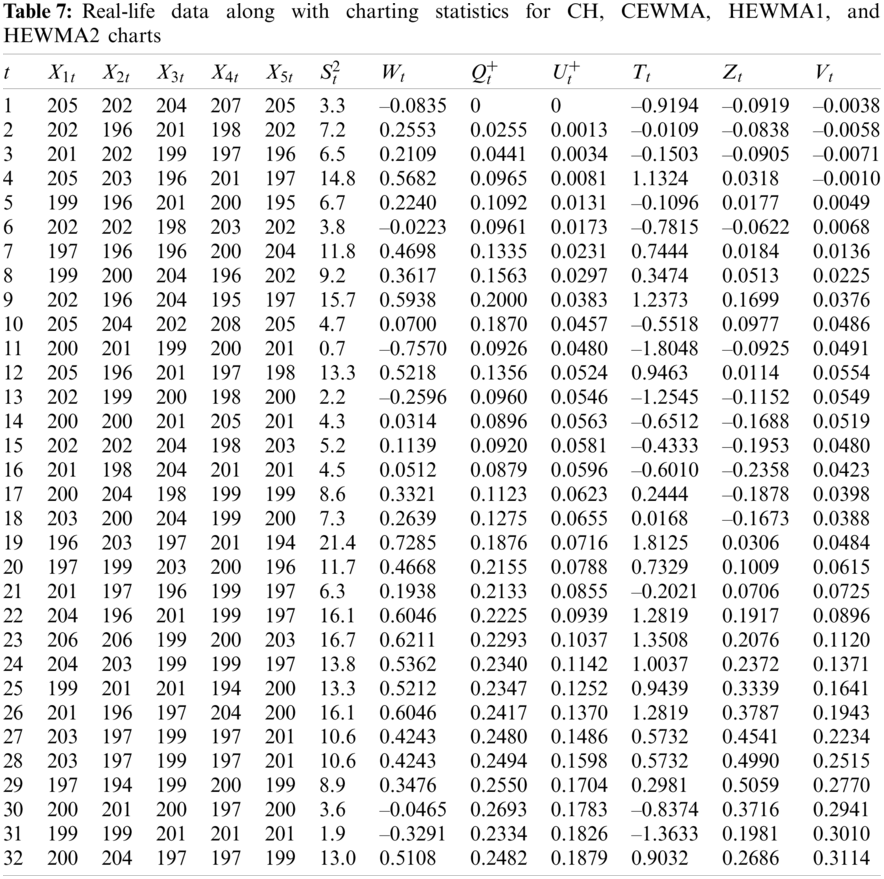
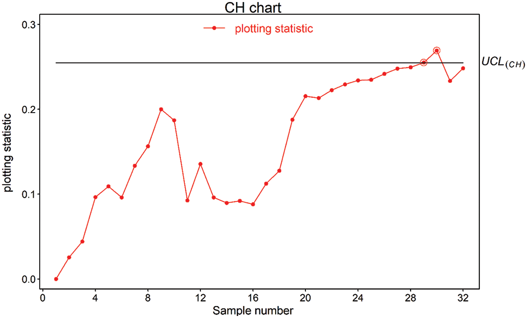
Figure 4: Real-life application of CH chart using
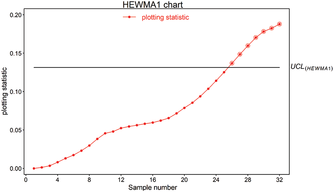
Figure 5: Real-life application of proposed HEWMA1 chart using
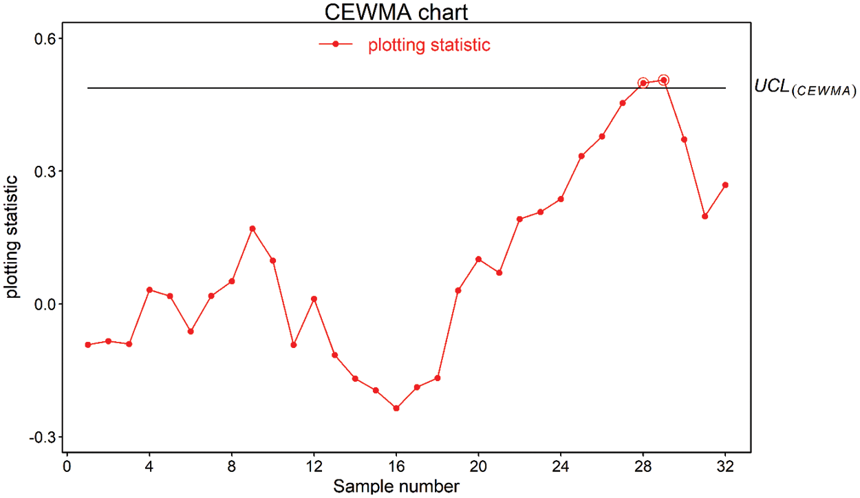
Figure 6: Real-life application of CEWMA chart using
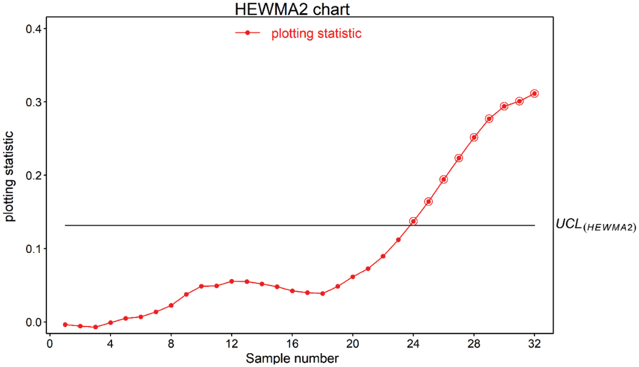
Figure 7: Real-life application of proposed HEWMA2 chart using
This paper proposes two new hybrid EWMA charts to monitor the shifts in the process variance. The proposed charts are called HEWMA1 and HEWMA2 charts. The HEWMA1 chart is designed using the CH statistic as the input for the HEWMA1 statistic, while in the same lines, CEWMA statistic is used as the input for the HEWMA2 statistic to construct the proposed HEWMA2 chart. In order to evaluate the performance of the proposed HEWMA1 and HEWMA2 charts, the extensive Monte Carlo simulation approach is used to approximate the run length properties, including the average run length and standard deviation run length. Similarly, to assess the overall performances of the proposed HEWMA1 and HEWMA2 charts, the extra quadratic loss, relative average run length, and performance comparison index are computed. The proposed HEWMA1 and HEWMA2 charts are compared to existing CH, CEWMA, HEWMA, AEWMA, HHW1, HHW2, AIBEWMA1, and AIBEWMA2 charts, and the comparison indicates that the proposed HEWMA1 and HEWMA2 charts outperform the existing charts. In the end, real-life data are analyzed to enhance the efficiency of the proposed HEWMA1 and HEWMA2 charts.
Funding Statement: 2019 Shanxi Province Soft Science Research Program Project ``Research on Sustainable Development Capacity and Classification Construction of Shanxi Development Zone'' (Project No. 2019041005-2).
Conflicts of Interest: The authors declare that they have no conflicts of interest to report regarding the present study.
1. Ajadi, J. O., Riaz, M., Al-Ghamdi, K. (2016). On increasing the sensitivity of mixed EWMA-CUSUM control charts for location parameter. Journal of Applied Statistics, 43(7), 1262–1278. DOI 10.1080/02664763.2015.1094453. [Google Scholar] [CrossRef]
2. Montgomery, D. C. (2012). Introduction to statistical quality control. New York: John Willey & Sons. [Google Scholar]
3. Roberts, S. (1959). Control chart tests based on geometric moving averages. Technometrics, 1(3), 239–250. DOI 10.1080/00401706.1959.10489860. [Google Scholar] [CrossRef]
4. Hunter, J. S. (1986). The exponentially weighted moving average. Journal of Quality Technology, 18(4), 203–210. DOI 10.1080/00224065.1986.11979014. [Google Scholar] [CrossRef]
5. Crowder, S. V. (1987). A simple method for studying run-length distributions of exponentially weighted moving average charts. Technometrics, 29(4), 401–407. DOI 10.2307/1269450. [Google Scholar] [CrossRef]
6. Crowder, S. V. (1989). Design of exponentially weighted moving average schemes. Journal of Quality Technology, 21(3), 155–162. DOI 10.1080/00224065.1989.11979164. [Google Scholar] [CrossRef]
7. Lucas, J. M., Saccucci, M. S. (1990). Exponentially weighted moving average control schemes—Properties and enhancements. Technometrics, 32(1), 1–12. DOI 10.1080/00401706.1990.10484583. [Google Scholar] [CrossRef]
8. Haq, A. (2013). A new hybrid exponentially weighted moving average control chart for monitoring process mean. Quality and Reliability Engineering International, 29(7), 1015–1025. DOI 10.1002/qre.1453. [Google Scholar] [CrossRef]
9. Abbas, N., Riaz, M., Does, R. J. (2014). Memory-type control charts for monitoring the process dispersion. Quality and Reliability Engineering International, 30(5), 623–632. DOI 10.1002/qre.1514. [Google Scholar] [CrossRef]
10. Ali, R., Haq, A. (2018). A mixed GWMA-CUSUM control chart for monitoring the process mean. Communications in Statistics—Theory and Methods, 47(15), 3779–3801. DOI 10.1080/03610926.2017.1361994. [Google Scholar] [CrossRef]
11. Tang, A., Sun, J., Hu, X., Castagliola, P. (2019). A new nonparametric adaptive EWMA control chart with exact run length properties. Computers & Industrial Engineering, 130(3), 404–419. DOI 10.1016/j.cie.2019.02.045. [Google Scholar] [CrossRef]
12. Haq, A. (2019). A new nonparametric synthetic EWMA control chart for monitoring process mean. Communications in Statistics—Simulation and Computation, 48(6), 1665–1676. DOI 10.1080/03610918.2017.1422750. [Google Scholar] [CrossRef]
13. Rasheed, Z., Zhang, H., Anwar, S. M., Zaman, B. (2021). Homogeneously mixed memory charts with application in the substrate production process. Mathematical Problems in Engineering, 2021, 1–15. DOI 10.1155/2021/2582210. [Google Scholar] [CrossRef]
14. Rasheed, Z., Zhang, H., Arslan, M., Zaman, B., Anwar, S. M. et al. (2021). An efficient robust nonparametric triple EWMA Wilcoxon signed-rank control chart for process location. Mathematical Problems in Engineering, 2021(4), 1–28. DOI 10.1155/2021/2570198. [Google Scholar] [CrossRef]
15. Domangue, R., Patch, S. C. (1991). Some omnibus exponentially weighted moving average statistical process monitoring schemes. Technometrics, 33(3), 299–313. DOI 10.1080/00401706.1991.10484836. [Google Scholar] [CrossRef]
16. Crowder, S. V., Hamilton, M. D. (1992). An EWMA for monitoring a process standard deviation. Journal of Quality Technology, 24(1), 12–21. DOI 10.1080/00224065.1992.11979369. [Google Scholar] [CrossRef]
17. Shu, L., Jiang, W. (2008). A new EWMA chart for monitoring process dispersion. Journal of Quality Technology, 40(3), 319–331. DOI 10.1080/00224065.2008.11917737. [Google Scholar] [CrossRef]
18. Huwang, L., Huang, C. J., Wang, Y. H. T. (2010). New EWMA control charts for monitoring process dispersion. Computational Statistics & Data Analysis, 54(10), 2328–2342. DOI 10.1016/j.csda.2010.03.011. [Google Scholar] [CrossRef]
19. Castagliola, P. (2005). A new S2-EWMA control chart for monitoring the process variance. Quality and Reliability Engineering International, 21(8), 781–794. DOI 10.1002/(ISSN)1099-1638. [Google Scholar] [CrossRef]
20. Chang, T. C., Gan, F. F. (1994). Optimal designs of one-sided EWMA charts for monitoring a process variance. Journal of Statistical Computation and Simulation, 49(1--2), 33–48. DOI 10.1080/00949659408811559. [Google Scholar] [CrossRef]
21. Razmy, A. M., Peiris, T. S. G. (2015). Design of exponentially weighted moving average chart for monitoring standardized process variance. International Journal of Engineering & Technology, 13(5), 74–78. [Google Scholar]
22. Haq, A. (2017). New EWMA control charts for monitoring process dispersion using auxiliary information. Quality and Reliability Engineering International, 33(8), 2597–2614. DOI 10.1002/qre.2220. [Google Scholar] [CrossRef]
23. Ali, R., Haq, A. (2017). New memory-type dispersion control charts. Quality and Reliability Engineering International, 33(8), 2131–2149. DOI 10.1002/qre.2174. [Google Scholar] [CrossRef]
24. Saghir, A., Aslam, M., Faraz, A., Ahmad, L., Heuchenne, C. (2020). Monitoring process variation using modified EWMA. Quality and Reliability Engineering International, 36(1), 328–339. DOI 10.1002/qre.2576. [Google Scholar] [CrossRef]
25. Zaman, B., Lee, M. H., Riaz, M., Abujiya, M. R. (2019). An adaptive approach to EWMA dispersion chart using Huber and Tukey functions. Quality and Reliability Engineering International, 35(6), 1542–1581. DOI 10.1002/qre.2460. [Google Scholar] [CrossRef]
26. Riaz, M., Abbasi, S. A., Abid, M., Hamzat, A. K. (2020). A new HWMA dispersion control chart with an application to wind farm data. Mathematics, 8(12), 2136. DOI 10.3390/math8122136. [Google Scholar] [CrossRef]
27. Chatterjee, K., Koukouvinos, C., Lappa, A. (2020). A new S2-TEWMA control chart for monitoring process dispersion. Quality and Reliability Engineering International, 37(4), 1334–1354. DOI 10.1002/qre.2798. [Google Scholar] [CrossRef]
28. Haq, A. (2016). A new hybrid exponentially weighted moving average control chart for monitoring process mean: Discussion. Quality and Reliability Engineering International, 33(7), 1629–1631. DOI 10.1002/qre.2092. [Google Scholar] [CrossRef]
29. Aslam, M., Azam, M., Khan, N., Jun, C. H. (2015). A control chart for an exponential distribution using multiple dependent state sampling. Quality & Quantity, 49(2), 455–462. DOI 10.1007/s11135-014-0002-2. [Google Scholar] [CrossRef]
30. Aslam, M., Khan, N., Jun, C. (2016). A hybrid exponentially weighted moving average chart for COM-Poisson distribution. Transactions of the Institute of Measurement and Control, 40(2), 456–461. DOI 10.1177/0142331216659920. [Google Scholar] [CrossRef]
31. Aslam, M., Azam, M., Jun, C. H. (2018). A HEWMA-CUSUM control chart for the Weibull distribution. Communications in Statistics—Theory and Methods, 47(24), 5973–5985. DOI 10.1080/03610926.2017.1404100. [Google Scholar] [CrossRef]
32. Noor-ul-Amin, M., Khan, S., Sanaullah, A. (2019). HEWMA control chart using auxiliary information. Iranian Journal of Science and Technology, Transactions A: Science, 43(3), 891–903. DOI 10.1007/s40995-018-0585-x. [Google Scholar] [CrossRef]
33. Aslam, M., Rao, G. S., AL-Marshadi, A. H., Jun, C. H. (2019). A nonparametric HEWMA-p control chart for variance in monitoring processes. Symmetry, 11(3), 356. DOI 10.3390/sym11030356. [Google Scholar] [CrossRef]
34. Noor, S., Noor-ul-Amin, M., Mohsin, M., Ahmed, A. (2020). Hybrid exponentially weighted moving average control chart using Bayesian approach. Communications in Statistics—Theory and Methods. DOI 10.1080/03610926.2020.1805765. [Google Scholar] [CrossRef]
35. Asif, F., Khan, S., Noor-ul-Amin, M. (2020). Hybrid exponentially weighted moving average control chart with measurement error. Iranian Journal of Science and Technology, Transactions A: Science, 44(3), 801–811. DOI 10.1007/s40995-020-00879-3. [Google Scholar] [CrossRef]
36. Noor-Ul-Amin, M., Shabbir, N., Khan, N., Riaz, A. (2020). Hybrid exponentially weighted moving average control chart for mean using different ranked set sampling schemes. Kuwait Journal of Science, 47(4), 19–28. [Google Scholar]
37. Lawless, J. F. (2003). Statistical models and methods for lifetime data. New Jersey: John Wiley and Sons. [Google Scholar]
38. Quesenberry, C. P. (1995). On properties of Q charts for variables. Journal of Quality Technology, 27(3), 184–203. DOI 10.1080/00224065.1995.11979592. [Google Scholar] [CrossRef]
39. Awais, M., Haq, A. (2018). A new cumulative sum control chart for monitoring the process mean using varied L ranked set sampling. Journal of Industrial and Production Engineering, 35(2), 74–90. DOI 10.1080/21681015.2017.1417787. [Google Scholar] [CrossRef]
40. Aslam, M., Anwar, S. M. (2020). An improved Bayesian Modified-EWMA location chart and its applications in mechanical and sport industry. PLoS One, 15(2), e0229422. DOI 10.1371/journal.pone.0229422. [Google Scholar] [CrossRef]
41. Zafar, R. F., Abbas, N., Riaz, M., Hussain, Z. (2014). Progressive variance control charts for monitoring process dispersion. Communications in Statistics-Theory and Methods, 43(23), 4893–4907. DOI 10.1080/03610926.2012.717668. [Google Scholar] [CrossRef]
42. Anwar, S. M., Aslam, M., Riaz, M., Zaman, B. (2020). On mixed memory control charts based on auxiliary information for efficient process monitoring. Quality and Reliability Engineering International, 36(6), 1949–1968. DOI 10.1002/qre.2667. [Google Scholar] [CrossRef]
43. Ou, Y., Wu, Z., Tsung, F. (2012). A comparison study of effectiveness and robustness of control charts for monitoring process mean. International Journal of Production Economics, 135(1), 479–490. DOI 10.1016/j.ijpe.2011.08.026. [Google Scholar] [CrossRef]
44. Anwar, S. M., Aslam, M., Ahmad, S., Riaz, M. (2019). A modified-mxEWMA location chart for the improved process monitoring using auxiliary information and its application in wood industry. Quality Technology & Quantitative Management, 17, 561–579. [Google Scholar]
45. Haq, A. (2018). A new adaptive EWMA control chart for monitoring the process dispersion. Quality and Reliability Engineering International, 34(5), 846–857. DOI 10.1002/qre.2294. [Google Scholar] [CrossRef]
46. Zaman, B., Lee, M. H., Riaz, M., Abujiya, M. R. (2017). An adaptive EWMA scheme-based CUSUM accumulation error for efficient monitoring of process location. Quality and Reliability Engineering International, 33(8), 2463–2482. DOI 10.1002/qre.2203. [Google Scholar] [CrossRef]
47. Zaman, B. (2021). Efficient adaptive CUSUM control charts based on generalized likelihood ratio test to monitor process dispersion shift. Quality and Reliability Engineering International, 37(8), 3192–3220. DOI 10.1002/qre.2903. [Google Scholar] [CrossRef]
48. Abbas, N., Riaz, M., Does, R. J. M. M. (2013). CS-EWMA chart for monitoring process dispersion. Quality and Reliability Engineering International, 29(5), 653–663. DOI 10.1002/qre.1414. [Google Scholar] [CrossRef]
49. Anwar, S. M., Aslam, M., Zaman, B., Riaz, M. (2021). Mixed memory control chart based on auxiliary information for simultaneously monitoring of process parameters: An application in glass field. Computers & Industrial Engineering, 156(3), 107284. DOI 10.1016/j.cie.2021.107284. [Google Scholar] [CrossRef]
50. Anwar, S. M., Aslam, M., Zaman, B., Riaz, M. (2022). An enhanced double homogeneously weighted moving average control chart to monitor process location with application in automobile field. Quality and Reliability Engineering International, 38, pp. 174–194. DOI 10.1002/qre.2966. [Google Scholar] [CrossRef]
 | This work is licensed under a Creative Commons Attribution 4.0 International License, which permits unrestricted use, distribution, and reproduction in any medium, provided the original work is properly cited. |