Computer Modeling in Engineering & Sciences

DOI: 10.32604/cmes.2022.020377

ARTICLE

A Cell-Based Linear Smoothed Finite Element Method for Polygonal Topology Optimization

Changkye Lee1, Sundararajan Natarajan2, Seong-Hoon Kee3 and Jurng-Jae Yee3,*

1University Core Research Center for Disaster-Free & Safe Ocean City Construction, Dong-A University, Busan, 49315, Korea
2Department of Mechanical Engineering, Indian Institute of Technology Madras, Chennai, 600036, India
3Department of Architectural Engineering, Dong-A University, Busan, 49315, Korea
*Corresponding Author: Jurng-Jae Yee. Email: jjyee@dau.ac.kr
Received: 22 November 2021; Accepted: 13 December 2021

1  Introduction

The structural topology optimization is playing the role as one of the effective tools to seek an optimal material distribution within a given domain showing the best structural performance [1]. Since the inception of homogenization method by Bendsøe et al. [2], a variety of topology optimization schemes have been introduced, viz. solid isotropic material with penalization (often called SIMP) [3–5], evolutionary structural optimization (ESO) [6] and level-set method [7,8], to name a few. Among these approaches, SIMP technique, in particular, is popular due to its ease of implementation; thus, it embraces a wide area of engineering fields [9]. To tackle a specific design domain in engineering fields, a reliable discretization of the domain is required, which is supplemented with design variables and appropriate constraint conditions. Due to its robustness, the finite element method (FEM) is employed to structural optimization. In FEM, typically lower-order triangular or quadrilateral cells are used. A triangular finite element cell is easy to use but its performance is not high as quadrilaterals. On the other hand, a quadrilateral cell provides relatively better results compared to triangles; yet, it often meets difficulty to generate meshes for very complex problem domains. In addition, it is known that quadrilateral finite elements may cause a rotational mesh-dependency [10]. To alleviate these difficulties, one viable alternative is to relax the mesh topology constraint, by employing element with arbitrary number of sides within the framework of the polygonal finite element method.

Not only polytopes show great flexibility in meshing the geometrically complex-shaped problem domains, but also are able to produce more accurate solutions than the standard triangular/quadrilateral finite element cells [11]. An attempt to topology optimization with polygonal cells is introduced by Talischi et al. [10]. Then, they developed a Matlab code of the polygonal mesh generator for a general purpose [12] to deliver an effective polygonal topology optimization [13,14]. Polygonal topology optimization is extended to fluid flow optimization [15], dynamics [16] and polytree-enhancement [11].

Meanwhile, an endeavour to improve the quality of triangular cells has undertaken to bring its convenience of mesh generation. Strain smoothing approach (so called S-FEM) [17–19] has received notable attention as a reliable candidate to overcome difficulties of triangles, viz. over-estimation of the stiffness and sensitivity to distorted meshes. This strain smoothing approach has been widely employed to manifold engineering fields, for instance, nonlinear elasticity [20], coupled with XFEM [21] and hybrid/enrichment [20,22]. A recent application to polytopes by Francis et al. [23,24] shows that strain-smoothed approach offers accurate and high performance in solution compared to both standard FEM and S-FEM. The salient features of S-FEM are: (a) does not require the gradient of the shape functions to compute the bilinear/linear form and (b) avoids Jacobian and iso-parametric mapping which lead to tolerate severe mesh distortion. Further, this scheme is relatively easy to implement to the existing FE codes with little modifications. In this study, the SIMP method is utilized within the framework of the cell-based linear smoothed finite element method for the sake of its computational reliability and robustness. The gradients are smoothed over the smoothing domains with a linear polynomial weight function, which is then employed to compute the stiffness. Materials are allocated on each smoothing domain and the weight function for the sensitivity filter is also defined to smoothing domain-based by the distance between each the smoothing domains. For this reason, the proposed strain smoothing topology optimization is fully smoothing domain dependent unlike the polyFEM.

This paper is organized as follows: Governing equations for linear solid elastic problems are briefly revisited in Section 2. Then, cell-based linear smoothed finite element approximation in the context of a polygonal finite element cell is introduced in Section 3. In the Section 4, the structural topology optimization within cell-based strain smoothing approach is explained. A few numerical examples are investigated in Section 5 to demonstrate the performance of the proposed scheme and followed by conclusion section.

2  Governing Equations

Consider an elastic body occupying Ω∈Rd and it is bounded by (d −1)-dimensional surface. The boundary is assumed the following decomposition: Γ=Γu∪Γt and ∅=Γu∩Γt, where Dirichlet boundary Γu and Neumann boundary Γt. The boundary-value problem for linear elastostatic is: find u:Ω→Rd:

∇⋅σ=f,∀x∈Ωu=u^,∀x∈Γuσ⋅n=g,∀x∈Γt (1)

where σ is the Cauchy stress tensor, n is the unit outward normal f is the body force, and u^ and g are prescribed displacements and tractions on each Dirichlet boundary Γu and Neumann boundary Γt, respectively.

The following variational form is obtained from Eq. (1):

∫Ωσ⋅∇vdΩ=∫Ωf⋅vdΩ+∫ΓNg⋅vdΓ (2)

where the test function v.

The infinitesimal strain ε is given as:

ε=12(∇u+∇uT) (3)

and its relation to the stress is given as follows using Hooke’s law:

σ=Cε (4)

where C is the elasticity tensor.

Substituting Eqs. (3) and (4), Eq. (2) can be rewritten as:

∫ΩCε(uh)⋅(vh)dΩ=∫Ωf⋅vhdΩ+∫ΓNg⋅vhdΓ (5)

Then, the discrete form of Eq. (5) can be define by standard Bubnov-Galerkin procedure as follows:

Kuh=b (6)

where the stiffness K and the external force b are defined as:

K=∑h∫ΩhBTCBdΩb=∑h(∫ΩhΨTfdΩ+∫ΓNhΨTgdΓ) (7)

where the shape functions Ψ and the strain-displacement matrix from the derivatives of the shape functions B=∇sΨ, respectively.

3  Cell-Based Linear Smoothed Finite Element Approximation

In this section, the linear smoothing function in the framework of cell-based smoothed finite element method for polygonal finite element cells is briefly revisited. The infinitesimal strain tensor for smoothed strain approach on the smoothing domain Ωk with the smoothing function f(x) is defined as:

ε¯h(xk)=∫Ωkε(x)f(x)dΩ,∀x∈Ω (8)

In the standard strain smoothing approach, the smoothing function f is a constant f(x)=1. In general, this scheme is used for linear triangular or bilinear quadrilateral finite element cells. However, the constant smoothing function is not suitable for polygonal meshes [23]. Hence, an another treatment is required to use polygonal finite element in the framework of strain-smoothed scheme. Therefore, Francis et al. [23] proposed a linear smoothing function employing a polynomial basis function to the use of polygonal finite elements:

f(x)=[1,x1,x2]T (9)

and its derivative is f,j(x)=[0,δ1j,δ2j]T. Eq. (9) can be approximately defined as the following consistency [25]:

∑IΨI(x)=1,∑IΨI(x)XI=x,∑IΨI(x)YI=y (10)

where the sampling point is given as x={x,y} and Ψ is the shape functions. Then, Eq. (10) can be rewritten as follows:

f(x)=∑IΨI(x)f(xI) (11)

and its spatial derivative is obtained as:

f,a(x)=∑IΨI,a(x)f(xI) (12)

where for ΨI,1 and ΨI,2, respectively:

∑IΨI,1(x)=0,∑IΨI,1(x)XI=1,∑IΨI,1(x)YI=0∑IΨI,2(x)=0,∑IΨI,2(x)XI=0,∑IΨI,2(x)YI=1 (13)

The aforementioned procedure leads to yield the basis function derivative level: therefore, the RHS of Eq. (8) can be rewritten as [23,24]:

∫ΩkΨa,jf(x)dΩ=∫ΓkΨaf(x)njdΩ−∫ΩkΨaf,j(x)dΩ (14)

where Ωk is the sub-domain, Γk is the boundary of sub-domain, n is the outward unit normal vector and the shape functions Ψ for arbitrary complex polytopes are the following Wachspress functions.

Wachspress basis function for polytopes.

To generate shape functions of arbitrary polygons, Wachspress basis function [26] is used in this work. Wachspress introduced rational basis functions on arbitrary polygonal meshes that the algebraic equations of the edges are used to yield nodal interpolation and linearity on the boundaries. Later, Warren et al. [27] proposed the generalized Wachspress shape function for simplex convex polyhedral elements. For the interested readers, the detailed explanation of the use of Wachspress function for smoothed polygonal element cell can be found in [23,28]. A simple form of a barycentric Wachspress basis function for irregular n-sided polygons is given by Meyer et al. [29]:

Ψj(x)=wj(x)∑kwk(x) (15)

where

wj(x)=A(qj−1,qj,qj+1)A(qj−1,qj,p)A(qj,qj+1,p)=sin⁡(γj+δj)sin⁡(γj)sin⁡(δj)‖p−qj‖2=cot⁡(γj)+cot⁡(δj)‖p−qj‖2 (16)

where A(p,q,r) is the signed area of triangle (p,q,r), and γj and δj are adjacent angles as shown in Fig. 1. Note that, the Wachspress basis function shows the lowest shape function while presenting the boundedness, linearity and linear consistency on convex polytopes.

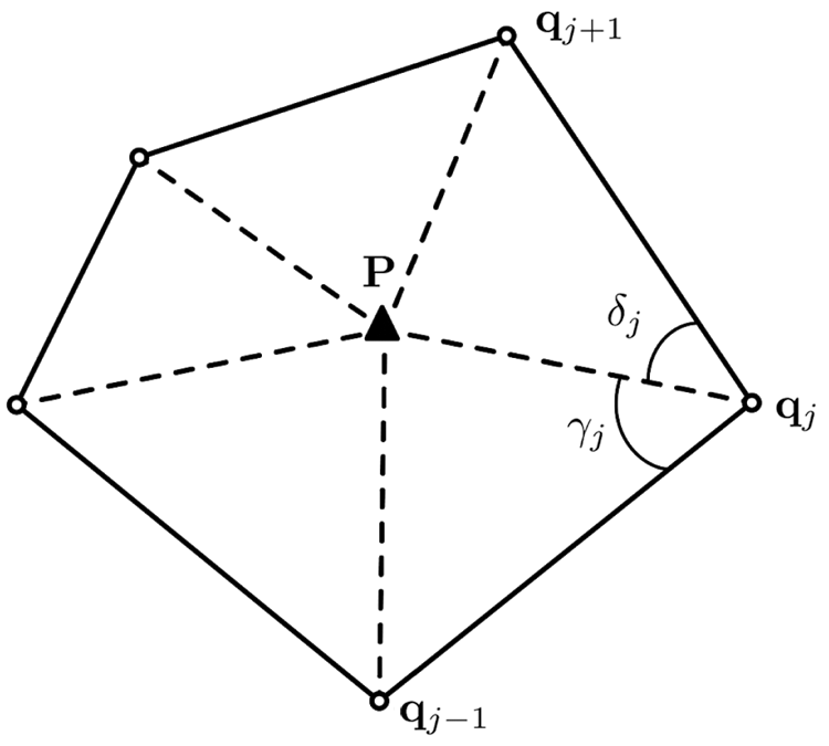
Figure 1: Barycentric coordinates for a polygon: the circle is a field node and the triangle is a centroid

Modified basis functions in the framework of linear smoothed finite element approximation.

The explicit form in two-dimension of Eq. (14) with the proposed the linear smoothing function can be explained as follows:

∫ΩkΨa,1dΩ=∫ΓkΨan1dΓ∫ΩkΨa,1(x1)dΩ=∫ΓkΨa(x1)n1dΓ−∫ΩkΨadΩ∫ΓkΨa,1(x2)dΩ=∫ΓkΨa(x2)n1dΓ (17)

and

∫ΩkΨa,2dΩ=∫ΓkΨan2dΓ∫ΩkΨa,2(x1)dΩ=∫ΓkΨa(x1)n2dΓ∫ΓkΨa,2(x2)dΩ=∫ΓkΨa(x2)n2dΓ−∫ΩkΨadΩ (18)

with the linear smoothing function derivatives f,1=[0,1,0] for Ψa,1 and f,2=[0,0,1] for Ψa,2.

As defined in Eqs. (17) and (18), the proposed approach requires two different numerical integration schemes: one on the boundaries of smoothing domains (Γk) and another in smoothing domain (Ωk). For the integration on the boundaries, the aforementioned Wachspress shape functions are used, whilst the Lagrangian basis functions are employed for interior integration scheme. Two integration schemes are illustrated in Fig. 2. As shown in Fig. 2, the polygonal finite element cell is sub-divided into five triangular sub-cells with geometric center O. As the same as the standard cell-based smoothed FEM, the target sub-cell is constructed as the smoothing domain in this approximation. Then, two Gaussian quadrature points are located on each boundary Γkn,n={1,2,3} of the smoothing domain Ωk. Three interior Gaussian quadrature points are in the smoothing domain Ωk to compute RHS of Eqs. (17) and (18). The two-dimensional matrix form of the outward normal vector n is given as:

n=[n100n2n2n1] (19)

Now, Eqs. (17) and (18) can be rewritten as the two-dimensional system of equations: WGaussdj=fj where j∈{1,2}. Gauss weights matrix WGauss and the vector fj are defined as:

WGauss=[1w2w3w1w1x12w2x13w3x11w1x22w2x23w3x2] (20)

and

f1=[∑k=13∑g=12Ψa(kgs)kn1kgv∑k=13∑g=12Ψa(kgs)kgs1kn1kgv−∑m=13Ψa(mr)mw∑k=13∑g=12Ψa(kgs)kgs2kn1kgv]f2=[∑k=13∑g=12Ψa(kgs)kn2kgv∑k=13∑g=12Ψa(kgs)kgs1kn2kgv∑k=13∑g=12Ψa(kgs)kgs2kn2kgv−∑m=13Ψa(mr)mw] (21)

where the coordinates of m-th interior Gauss points mr=(mr1,mr2) and their weights mw. The coordinates of k-th boundary Gauss points and their weights are given as kgs=(kgs1,kgs2) and kgv, respectively.

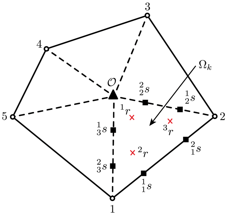
Figure 2: Numerical integration scheme of the smoothing domain for the linear smoothing function for the polygon. A ‘filled’ triangle is the geometric center of the polygon and ‘open’ circles are field nodes. The interior Gauss points where the modified shape functions are obtained are depicted as red crosses and Gauss points on the boundary of the smoothing domain are given as ‘filled’ squares

The j-th shape function derivatives vector dj, that is the modified shape functions and unknown vector in the present method, can be written as follows:

dj=[1dj,2dj,3dj]T=[Ψa,j(1r),Ψa,j(2r),Ψa,j(3r)]T (22)

and dj can be obtained at three internal Gauss points as follows:

dj=WGauss−1fj (23)

Then, the modified strain-displacement matrix can be evaluated as follows:

B¯(kr)=[B¯1(kr),B¯2(kr),…,B¯n(kr)] (24)

and the nodal strain-displacement matrix constructed at k-th internal Gauss point:

B¯a(kr)=[kd100kd2kd2kd1] (25)

where k∈{1,2,3}.

4  Solid Isotropic Materials with Penalization

In structural optimization, compliance c is minimized to attempt the optimal material distribution. To minimize the compliance, solid isotropic material with penalization (SIMP) method has gained massive attention among other topology optimization schemes, because of its use of fewer design variables and computation simplicity.

Therefore, the following power-law approach [30] is utilized in this paper to solve the problem in the context of the strain smoothing approximation:

minx:c(x)=UTK¯U=∑e=1NSD(xe)pueTK¯euesubject to:V(x)V0=Vf:K¯U=F:0<xmin≤x≤1 (26)

where compliance c is twice the strain energy obtained by corresponding displacements, U and ue are the global and element displacement, respectively. NSD is the number of cell-based smoothing domain and K¯ is the local smoothed stiffness matrix built over smoothing domains. The penalization power p=3.0∼9.0 (in particular, the penalization power p≥3.0 for Poisson’s ratio ν=0.3), the volume fraction Vf is the ratio of the material volume V(x) and the design variable x is in this work is the density. Note that, the relative density xmin is non-zero minimum value for the stability of simulation. The optimality criteria (OC) method [4] is employed to solve Eq. (22). The updated scheme using OC is given as follows [30,31]:

xek+1={max{(1−ζ)xe,xmin}ifxek(Bkek)η≤max{(1−ζ)xe,xmin}min{(1+ζ)xe,1}ifmin{(1+ζ)xe,1}≤xek(Bkek)ηxek(Bxek)ηotherwise (27)

A tuning parameter η and a move limit ζ are used as control parameters to obtain stable convergence [31]. Bxek, defined as Bxe at k-th iteration, can be written as:

Bxe=−∂c∂xeλ∂V∂xe (28)

where xe relies on the Lagrangian multiplier λ determined by a bisection method. Eq. (22) can be written in terms of the design variables only:

minx:c(xe)subject to:∑e=1NSDv~exe≤V~:0<xmin≤x≤1 (29)

where c(xe)=fTu and f=∑e=1NSDxepK¯eu. The compliance of Eq. (26) can be rewritten by adding the zero function:

c(x)=fTu−u~T(K¯u−f) (30)

where u~ is a fixed real vector whose value can be arbitrarily selected. Now we can derive Eq. (30) with respect to xe:

∂c∂xe=(fT−u~TK¯)∂u∂xe−u~T∂K¯∂xeu (31)

If fT−u~TK¯=0, Eq. (31) can be simplified as follows:

∂c∂xe=−u~T∂K¯∂xeu=−p(xe)p−1ueTK¯eue (32)

In the current approach, the smoothed stiffness matrix K¯ is obtained over each smoothing domain.

Now, the sensitivity filter is discussed. The density-based topology optimization often faced from the notorious checkerboard patterns [32]. Therefore, Bensøe et al. [31] introduced the following filter ensuring mesh-independency:

∂c^∂xe=1xe∑f=1NSDH^f∑f=1NSDH^fxf∂c∂xf (33)

where the weight function/mesh-dependent convolution operator H^f is defined as:

H^f=rmin−dist(e¯,f¯){f¯∈NSD|dist(e¯,f¯)≤rmin},e=1,…,NSD (34)

where dist(e¯,f¯) is the distance between the centroid of the smoothing domain e¯ and the centroid of the smoothing domain f¯. The weight function H^f is zero outside of the filter. Bendsøe and Sigmund suggested the minimum radius rmin of curvature 1+22d≈1.2d with the minimum length d. Fig. 3 shows the difference of filtering between the polyFEM and the proposed method. The overall optimization algorithm in the framework of the polyCS-FEM is presented in Fig. 4.

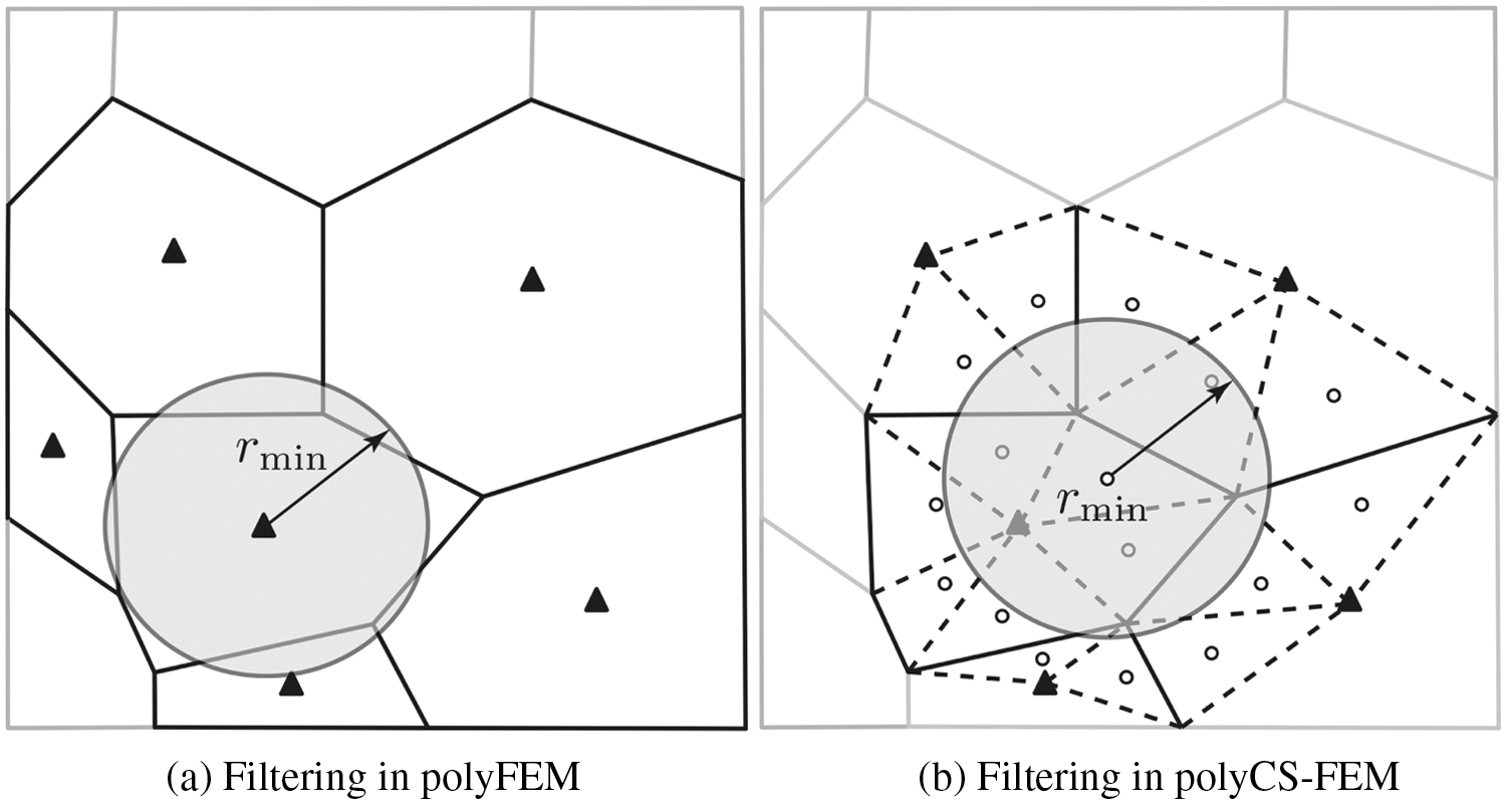
Figure 3: The filtering scheme comparison between poly FEM and the proposed linear smoothed CS-FEM: (a) polyFEM and (b) polyCS-FEM. Closed triangles are the centroid of each polygonal cell and open circles are the centroid of cell-based smoothing domains

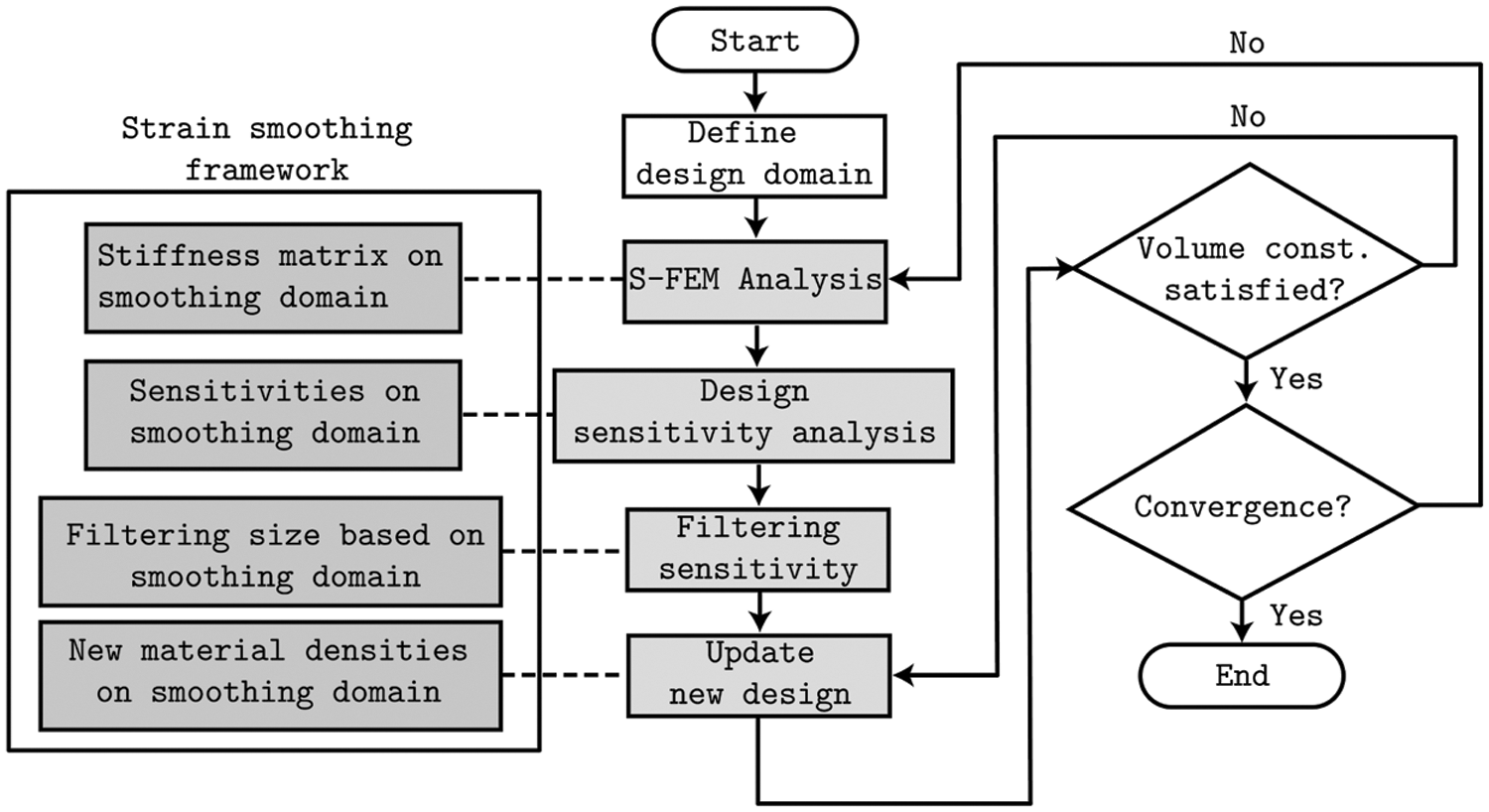
Figure 4: Topology optimization algorithm in the framework of the proposed linear smoothed cell-based strain smoothing scheme

5  Numerical Examples

In this section, a series of numerical tests are examined for the proposed topology optimization scheme. The domain is discretized with unstructured polygonal meshes using the open-source Matlab PolyMesher with builtin Matlab functions voronoin proposed by Talischi et al. [12]. The current approach is compared to results of topology optimization with polygonal finite element cells introduced by Talischi and co-workers [10,13]. A Matlab code for polygonal topology optimization written by Talischi et al. [13] is used as the reference solution to compare the performance of the current approach. The tuning parameter η=0.5 and move limits ζ=0.2 are often used for the rapid and stable convergence [31]. The other parameters for the optimization in the following numerical examples are the same as those used in the reference [13]. As the aforementioned, polygonal meshes are discretized to three-noded triangular sub-cells. Note that, the following examples are considered as dimensionless:

For discussing the results, the following convention is used:

•   polyFEM: conventional finite element method with polygonal cells;

•   polyCS-FEM: linear smoothing cell-based smoothed finite element method with polygonal cells;

•   BCs: boundary conditions;

•   DOFs: degrees-of-freedom.

5.1 Serpentine Beam

Firstly considering a Serpentine beam, for this test, the following control parameters are used: tuning parameter η=0.5, move limit ζ=0.2, the volume fraction Vf = 0.5 and the penalization power P = 3. Fig. 5 illustrates boundary conditions and a representative polygonal mesh generation which are used in this study. Young’s modulus E = 105 and Poisson’s ratio ν=0.3 are used as material properties in this section. The external concentrated force P = 1000 is imposed as shown in Fig. 5. Unstructured polygonal finite element are used with 10,136 DOFs.

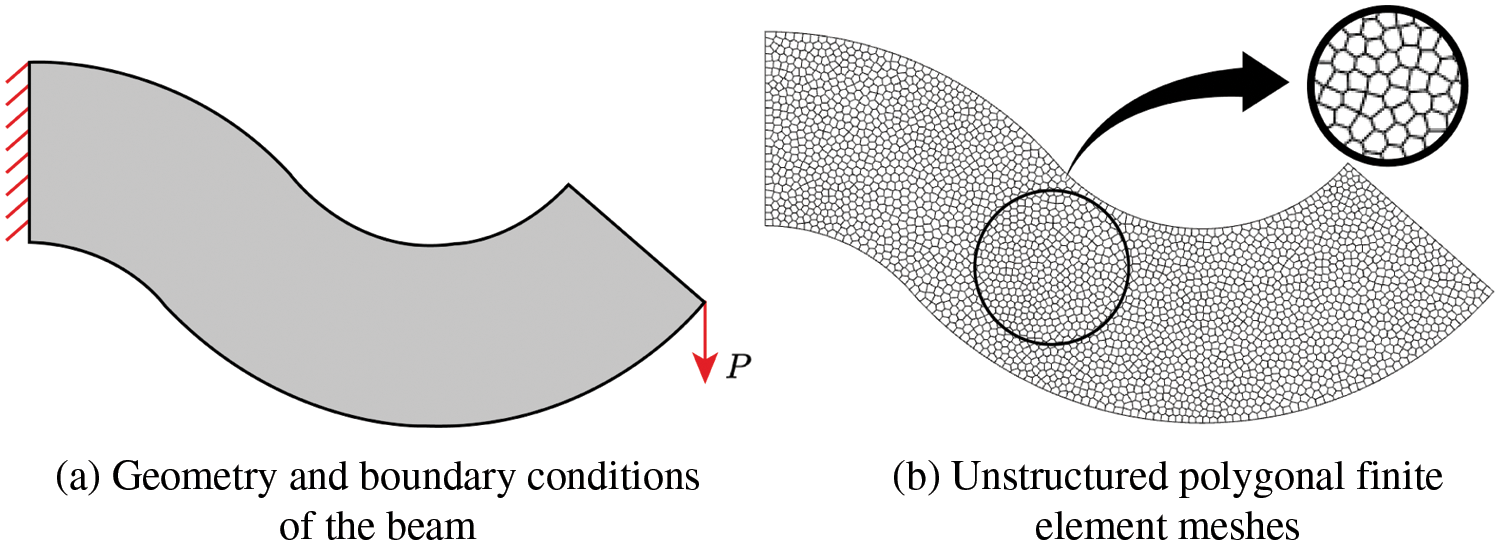
Figure 5: Boundary conditions and unstructured polygonal cells for Serpentine beam: (a) red solid line is Dirichlet BCs (fully constraint) and red arrow is the external force, and (b) unstructured polygonal finite element cells

Obtained optimized topologies of the polyFEM and polyCS-FEM for the Serpentine beam are shown in Fig. 6. The optimal topology of the proposed method is similar to its of Talischi et al. [13]. The rate of strain energy reduction and the corresponding values are provided in Fig. 7 and Table 1, respectively. For this test, the compliance reduce rate of the polyFEM is around 78%, while the polyCS-FEM is able to reduce only 77%, c=18.8572×103 to c = 419.84 with 86 iterations.

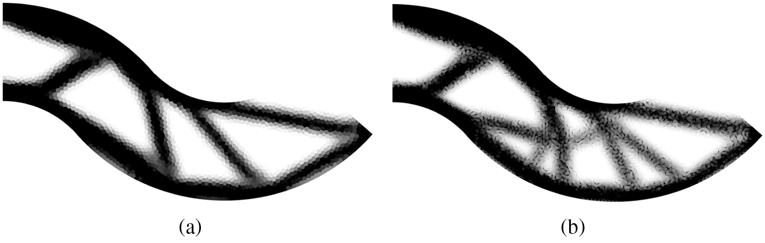
Figure 6: Optimized topologies of Serpentine beam: (a) polyFEM and (b) polyCS-FEM

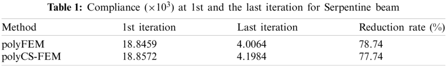
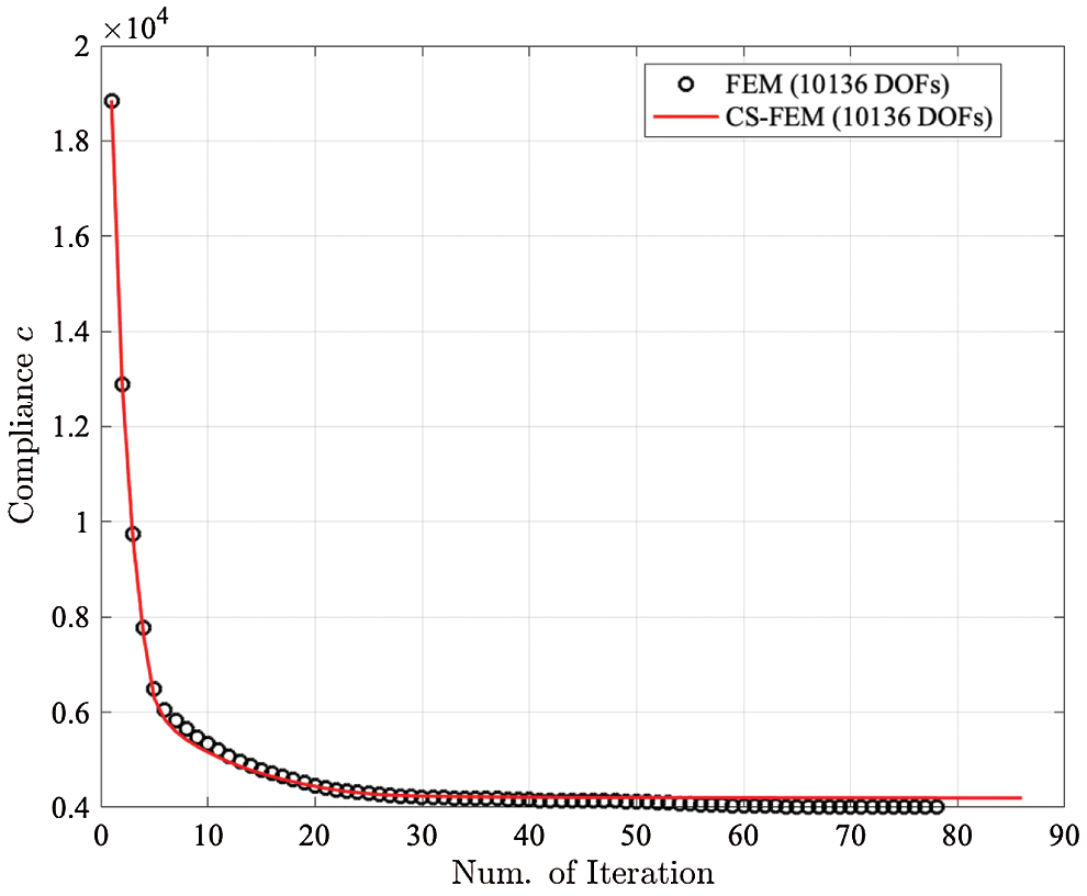
Figure 7: The rate of compliance convergence for Serpentine beam

5.2 Suspension Triangle

A suspension triangle is studied in this example. The corresponding boundary conditions and mesh discretization (10,178 DOFs) are given in Fig. 8. The same tuning parameter, move limit, volume fraction and penalization power as used in the previous example are utilized for this example. Isotropic material is assumed for Suspension triangle with Young’s modulus E = 105 and Poisson’s ratio ν=0.3. The external forces are implemented at the left lower point as the concentrated force P = 1000 (see Fig. 8).

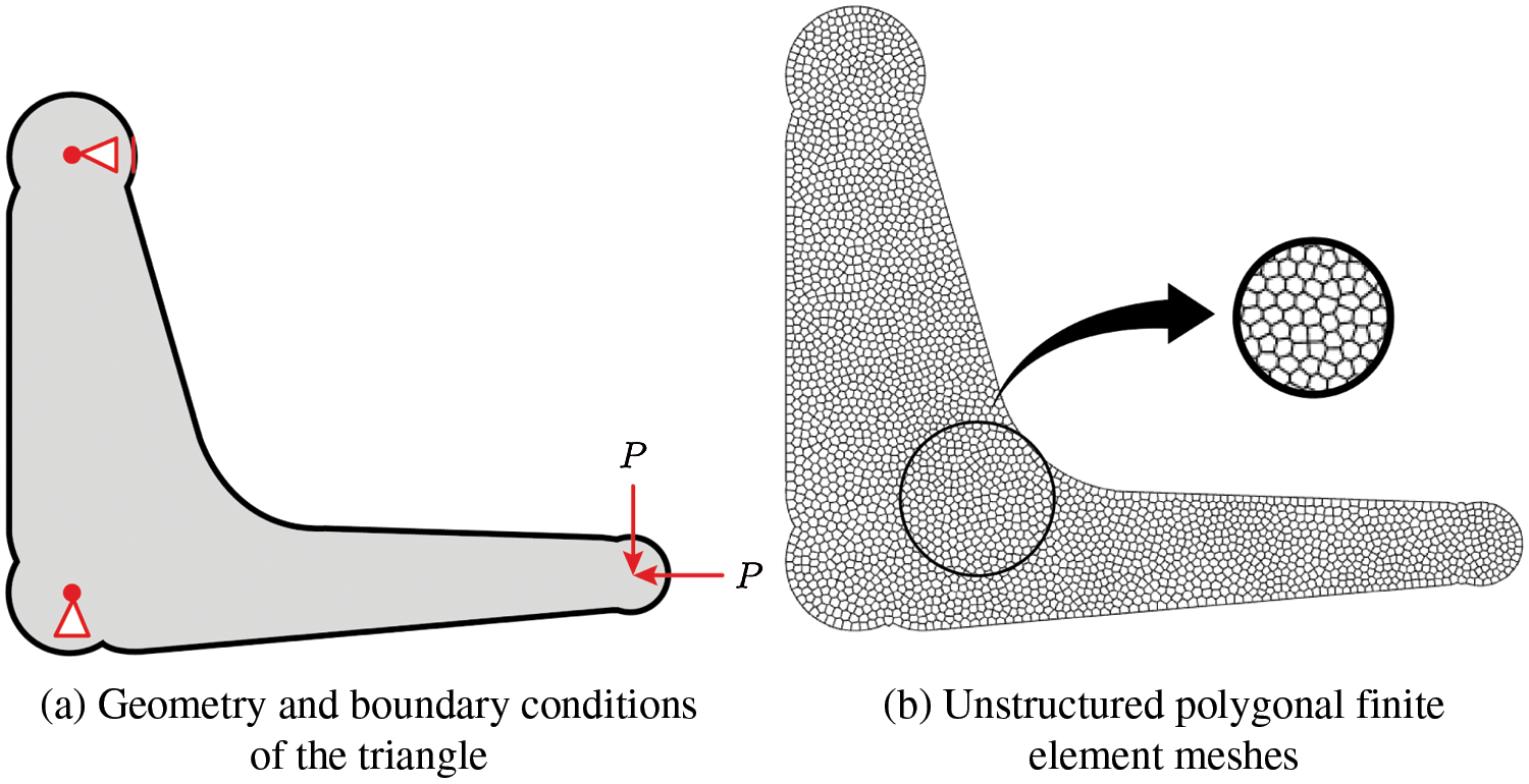
Figure 8: Boundary conditions and unstructured polygonal cells for Suspension triangle: (a) constraint to x-direction at the left upper point, fully constraint at the left lower point and red arrows are the external forces, and (b) unstructured polygonal finite element cells

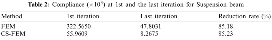
The optimized configurations for the suspension triangle derived from the polyFEM and polyCS-FEM are described in Fig. 9. A notable performance of the proposed scheme for this test is obtained as shown in Fig. 10 and Table 2 with the detailed values. After 165 iterations, value of 85.23% compliance reduction is observed by the current scheme.

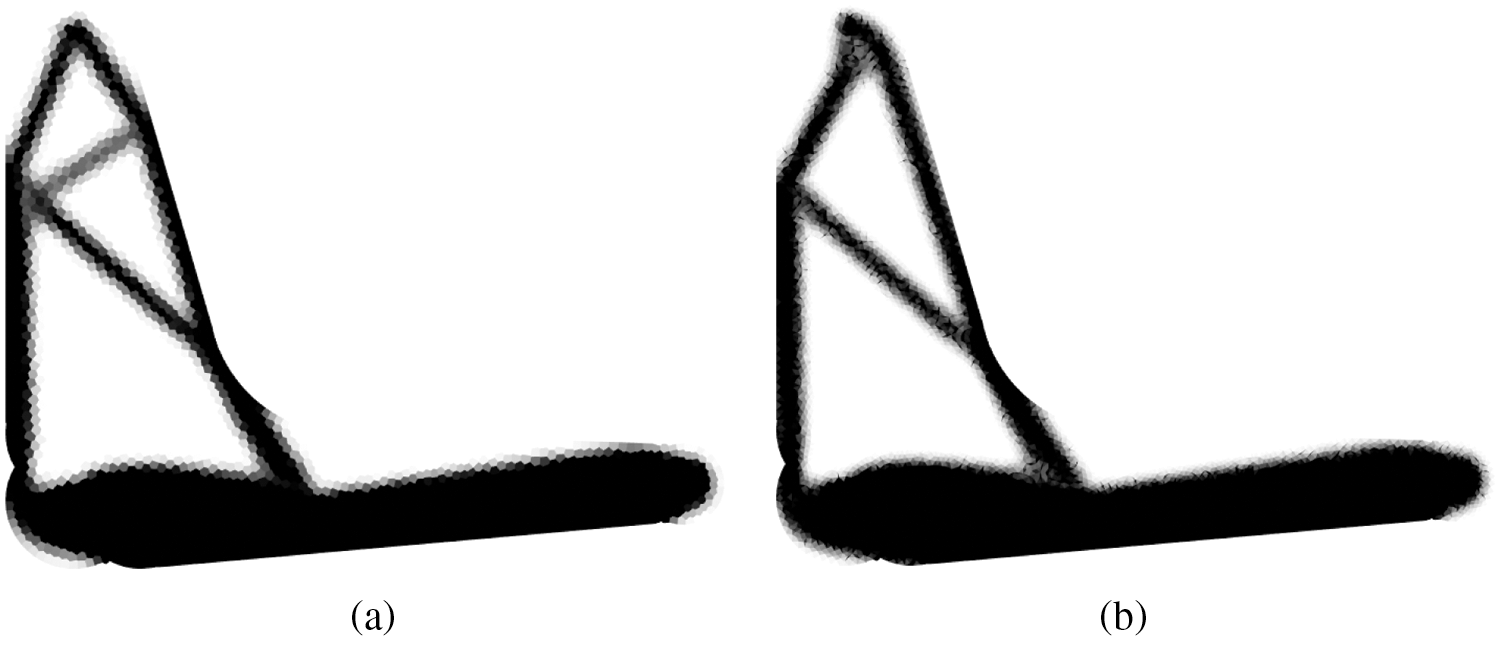
Figure 9: Optimized topologies of Suspension triangle: (a) polyFEM and (b) polyCS-FEM

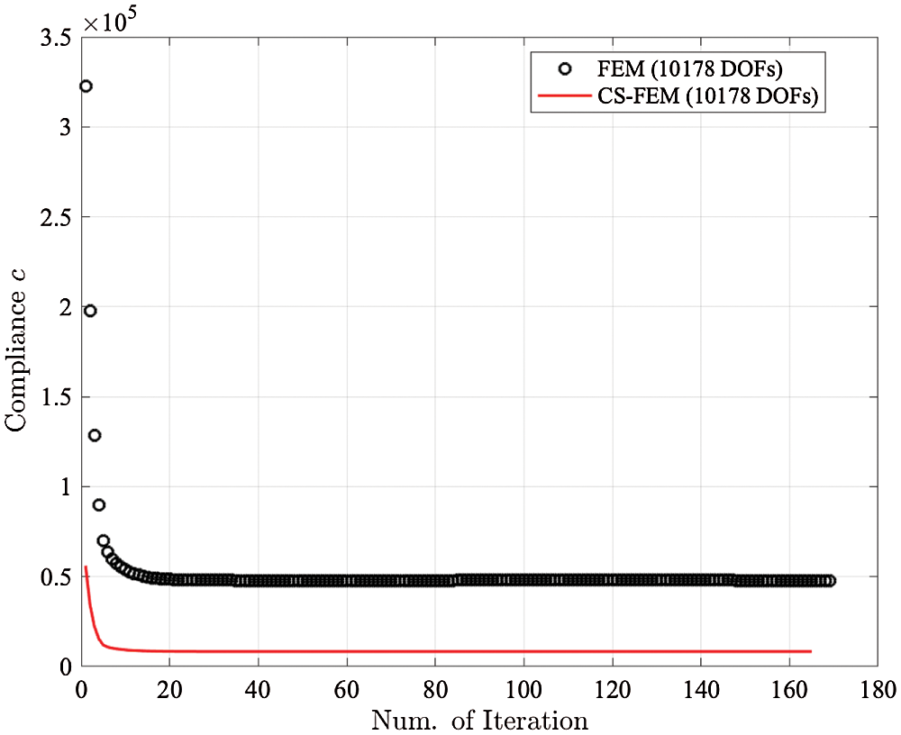
Figure 10: The rate of compliance convergence for Suspension triangle

5.3 Multiple Load Problem

Next, multiple load problem is investigated in this section. Michell beam is considered in this section with two loads P = 1000, the corresponding boundary conditions and a schematic spatial discretization with polygonal meshes which is equivalent to 10,128 DOFs are shown in Fig. 11. The following parameters are employed for the study: Tuning parameter η=0.4 and move limit ζ=0.2. The volume fraction for this method is set to Vf = 0.5 and the penalization power P = 3.

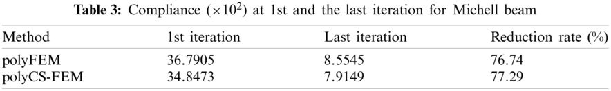
Fig. 12 represents the optimized topologies of Michell beam obtained by the polyFEM and the proposed cell-based linear S-FEM. As clearly shown in Fig. 12, the proposed approach shows smoother optimal topologies while some areas of the polyFEM have rather rough surfaces. The compliance convergence curve for both methods is given in Fig. 13 and the detailed compliance values are provided in Table 3. In the polyFEM, after 122 iterations, the strain energy is reduced from c = 3679.05 to c = 855.45 which is 76.75% reduction. In case of the proposed method, it achieves 77.29% strain energy reduction with 201 iterations. At the same level of iteration (which is 122), the polyCS-FEM is able to decrease the strain energy to c = 792.01.

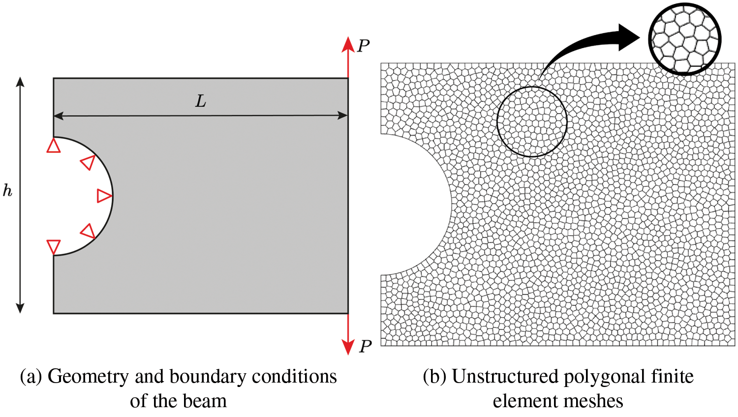
Figure 11: Michell beam problem: (a) geometry and boundary conditions and (b) unstructured polygonal finite element meshes

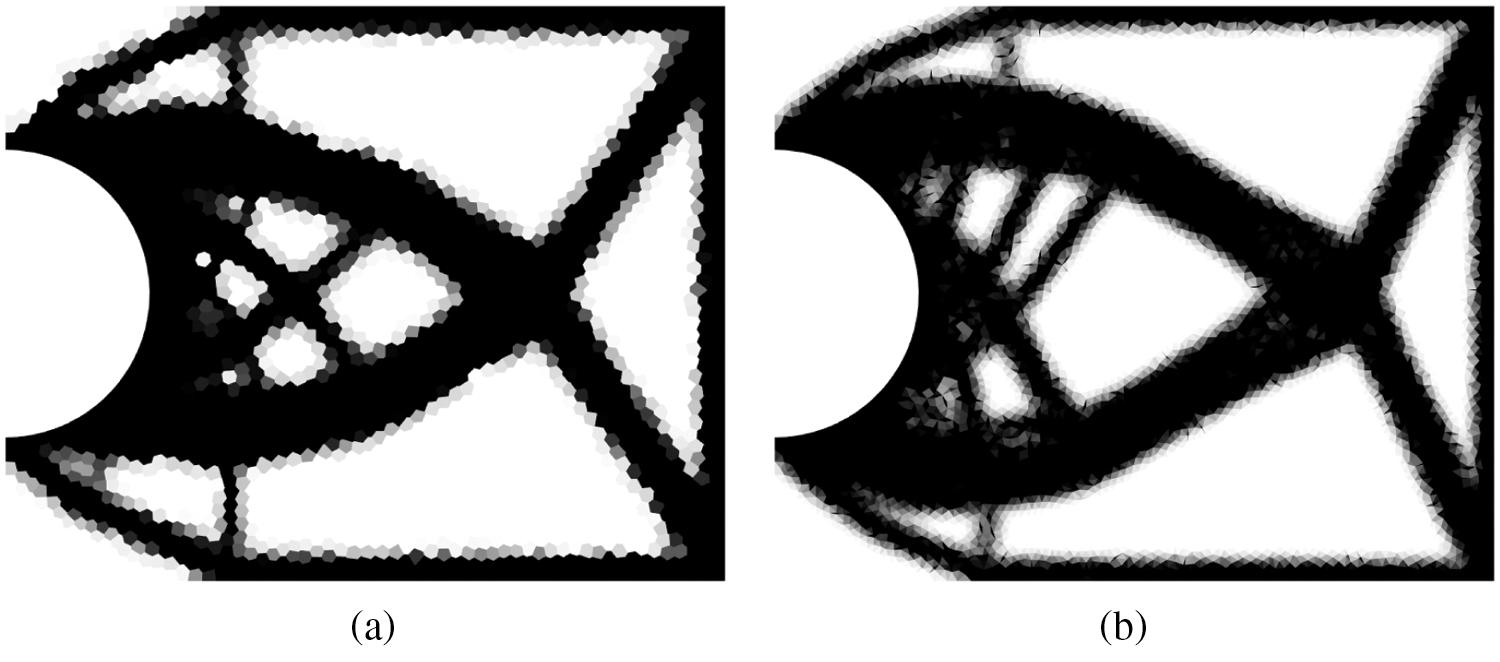
Figure 12: Optimized topologies of Michell beam: (a) polyFEM and (b) polyCS-FEM

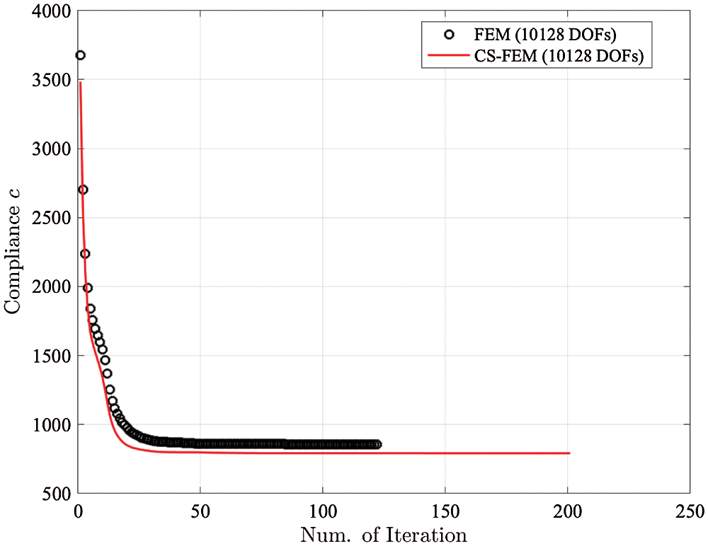
Figure 13: The rate of compliance convergence for Michell beam

5.4 Compliant Mechanism Synthesis

Lastly, a compliant mechanism synthesis problem is considered [33,34]. The domain of force inverter problem is [0,3]×[0,1] and unstructured polygonal meshes are discretized with 10,120 DOFs as shown in Fig. 14. Note that the given domain is only half of the whole domain since it is symmetrical. The following material properties are given as: Young’s modulus E = 1.0 and Poisson’s ratio ν=0.3. To minimize the negative horizontal output displacement, the input spring constant k1 = 0.1 and output spring constant k2 = 0.1 are utilized respectively. The volume is constrained to 30% with tuning parameter η=0.5 and move limit ζ=0.2. The penalization factor p = 3 is also used for this test. Fig. 15 shows the optimal topologies of polyFEM and polyCS-FEM. The convergence rate of the compliant mechanism design is given in Fig. 16. As shown in Fig. 16, the output displacements which are compliance in this example for each polyFEM and polyCS-FEM are obtained as: (a) c=0.0934∼−0.9918 for polyFEM and (b) c=0.0927∼−0.9187 for polyCS-FEM.

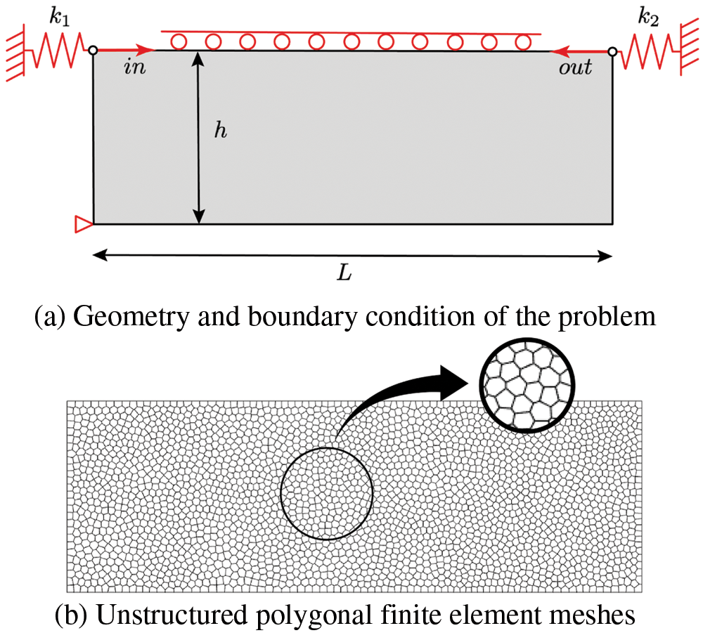
Figure 14: Optimized topologies of force inverter problem: (a) polyFEM and (b) polyCS-FEM

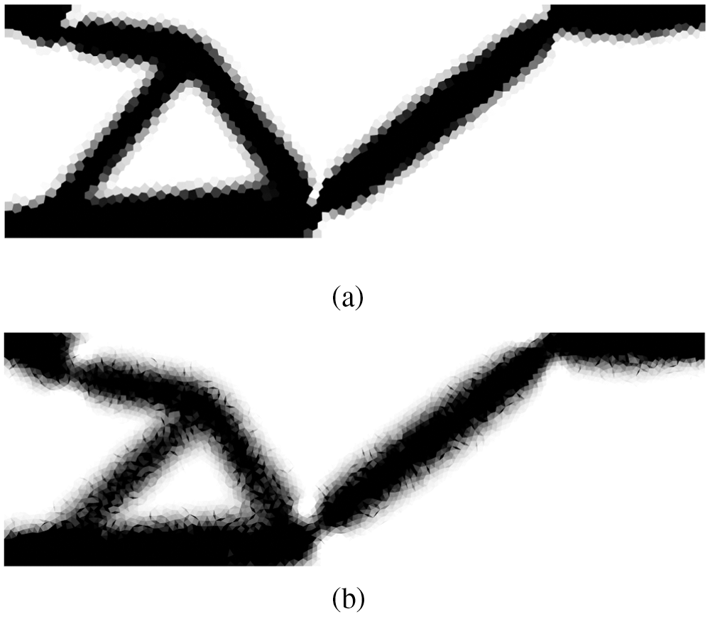
Figure 15: Optimized topologies of force inverter problem: (a) polyFEM and (b) polyCS-FEM

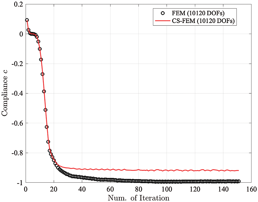
Figure 16: The rate of compliance convergence for force inverter problem

6  Conclusions

In this paper, the cell-based linear smoothed strain scheme for structural topology optimization and the method are presented. The proposed smoothed-strain framework has the following distinguishing features: (a) does not require the explicit form of shape functions and (b) two different boundary and interior integration schemes are employed. This leads to the standard CS-FEM can be utilized in polygonal finite element meshes. To use polygonal meshes in the context of smoothed finite element analysis, the polynomial basis function is employed as the smoothing function while it is a constant function in the standard S-FEM. The proposed polyCS-FEM requires two Gauss points on the boundaries of each smoothing domain and three interior Gauss points. Wachspress basis functions are used the inside of the smoothing domain to evaluate the shape function of the present approach. The smoothing domain-based filter is successfully incorporated into an optimization algorithm. From a set of numerical tests, the following conclusions can be drawn:

•   in general the polyCS-FEM needs more iterations to converge the compliance compared to the polyFEM because the bandwidth of the polyCS-FEM is wider than the polyFEM;

•   the polyCS-FEM provides the relatively smoother optimal topologies compared to polyFEM;

•   the polyCS-FEM is able to effectively yield compliance reduction rate even at the same level of iteration as the polyFEM.

To obtain the high resolution of optimal topologies, the employment of polytree meshes [35] will be considered as one of possible topics for the future communication.

Funding Statement: Changkye Lee, Seong-Hook Kee and Jurng-Jae Yee would like to thank the support by Basic Science Research Program through the National Research Foundation (NRF) funded by Korea Ministry of Education (No. 2016R1A6A1A0312812).

Conflicts of Interest: The authors declare that they have no conflicts of interest to report regarding the present study.

This work is licensed under a Creative Commons Attribution 4.0 International License, which permits unrestricted use, distribution, and reproduction in any medium, provided the original work is properly cited.