| Computer Modeling in Engineering & Sciences |
DOI: 10.32604/cmes.2022.018699
ARTICLE
Novel Time Series Bagging Based Hybrid Models for Predicting Historical Water Levels in the Mekong Delta Region, Vietnam
1Institute of Geography, Vietnam Academy of Science and Technology, Hanoi, 10000, Viet Nam
2Department of Civil, Environmental and Natural Resources Engineering, Lulea University of Technology, Lulea, 971 87, Sweden
3Institute of Geological Sciences, Vietnam Academy of Science and Technology (VAST), Dong Da, Hanoi, 10000, Viet Nam
4University of Transport Technology, Thanh Xuan, Ha Noi, 10000, Viet Nam
5Department of Watershed & Arid Zone Management, Gorgan University of Agricultural Sciences & Natural Resources, Gorgan, 4918943464, Iran
6DDG (R) Geological Survey of India, Gandhinagar, 382010, India
*Corresponding Authors: Nadhir Al-Ansari. Email: nadhir.alansari@ltu.se; Binh Thai Pham. Email: binhpt@utt.edu.vn
Received: 11 August 2021; Accepted: 27 September 2021
Abstract: Water level predictions in the river, lake and delta play an important role in flood management. Every year Mekong River delta of Vietnam is experiencing flood due to heavy monsoon rains and high tides. Land subsidence may also aggravate flooding problems in this area. Therefore, accurate predictions of water levels in this region are very important to forewarn the people and authorities for taking timely adequate remedial measures to prevent losses of life and property. There are so many methods available to predict the water levels based on historical data but nowadays Machine Learning (ML) methods are considered the best tool for accurate prediction. In this study, we have used surface water level data of 18 water level measurement stations of the Mekong River delta from 2000 to 2018 to build novel time-series Bagging based hybrid ML models namely: Bagging (RF), Bagging (SOM) and Bagging (M5P) to predict historical water levels in the study area. Performances of the Bagging-based hybrid models were compared with Reduced Error Pruning Trees (REPT), which is a benchmark ML model. The data of 19 years period was divided into 70:30 ratio for the modeling. The data of the period 1/2000 to 5/2013 (which is about 70% of total data) was used for the training and for the period 5/2013 to 12/2018 (which is about 30% of total data) was used for testing (validating) the models. Performance of the models was evaluated using standard statistical measures: Coefficient of Determination (R2), Root Mean Square Error (RMSE) and Mean Absolute Error (MAE). Results show that the performance of all the developed models is good (R2 > 0.9) for the prediction of water levels in the study area. However, the Bagging-based hybrid models are slightly better than another model such as REPT. Thus, these Bagging-based hybrid time series models can be used for predicting water levels at Mekong data.
Keywords: Computational techniques; bagging; water level; time series algorithms
Water level fluctuations are one of the common events on the earth, essentially because of the climate characteristics [1,2]. A flood can occur if a large amount of precipitation flows through the channels, overflowing the banks and submerging normal dry land [3,4]. Flood can be caused by heavy rainfall, rapid snowmelt, or a storm surge flooding inland and coastal areas. Thus, prediction of changes in water level of surface water bodies is one of the important tasks for water resources and flood management. However, the process of predicting water levels has always been one of the most complex issues in hydrology, which cannot be easily calculated by conventional methods such as NS_TIDE and auto-regressive method, which was used for short prediction of water levels in the Yangtze Estuary [5]. In addition, due to the lack of required information and the effect of many hydrological parameters on each other, the results obtained by these methods are not accurate enough and have high uncertainty. In the last two decades, artificial intelligent methods or Machine Learning (ML) methods have been used by many researchers in hydrological prediction and other hydrology studies [6–9]. The advantage of using these methods is the high and acceptable accuracy of results in a short time. Among ML models, Artificial Neural Network (ANN) models have been used in most cases for the short-term prediction. Neuro-fuzzy and neural network techniques were used for predicting sea level in Darwin Harbor, Australia [10]. In another study, the Support Vector Machines (SVM) model was used to predict water levels in the Lanyang River in Taiwan for short term (1 to 6 hrs) [11]. The SVM least squares method was also used in predicting medium- and long-term runoff [12]. Nguyen et al. [13] applied ML models such as LASSO, Random Forests and SVM to forecast daily water levels at Thakhek station on Mekong River. They concluded that SVM achieved feasible results (mean absolute error: 0. 486 m while the acceptable error of a flood forecast model required by the Mekong River Commission is between 0.5 and 0.75 m).
Nowadays, ensemble and hybrid models are being used in many fields including hydrology instead of single models to take advantage of combined capabilities of individual single models. A hybrid model ANFIS-SO which is a hybridization of Adaptive Neuro-Fuzzy Inference System (ANFIS) and Sunflower Optimization (SO) was successfully used to predict Urmia lake water levels in Iran [14]. Ghorbani et al. [15] developed a new hybrid model namely MLP-FFA, which is a combination of Multilayer Perceptron (MLP) and Firefly Algorithm (FFA), for prediction of water level in Lake Egirdir, Turkey. Yaseen et al. [16] developed a new hybrid model namely MLP-WOA, which is a combination of MLP and Whale Optimization Algorithm (WOA), for prediction of Van Lake water level fluctuation with monthly scale, and stated that the novel model MLP-WOA is a promising tool for the prediction of water level, and performance of this model was better than other ML models such as Self-Organizing Map (SOM), Random Forest Regression (RFR), Decision Tree Regression (DTR), Cascade-Correlation Neural Network Model (CCNNM), and classical MLP.
In general, the aforementioned studies showed and proved the superiority of the hybrid models compared with conventional models and single ML models in prediction of the water levels. Therefore, in this study, we have developed and used novel time series Bagging based hybrid models namely Bagging (RF), Bagging (SMO) and Bagging (M5P), which are a combination of the Bagging ensemble technique and different base predictors like Random Forest (RF), Sequential Minimal Optimization (SMO), and M5P for better prediction of the water levels at Mekong delta, Vietnam. Reduced Error Pruning Trees (REPT) as a benchmark ML model was used to compare with novel Bagging based hybrid models. The main difference and novelty of this study compared with previous works is that it is the first time these novel hybrid models are developed and applied for prediction of historical water levels, which can improve the accuracy of the water level prediction for better water resource management. The daily surface water level data from 18 water level measurement stations located in the Mekang delta, Vietnam for the 19 years period (2000 to 2018) was used for the model’s study. Various standard validation indicators such as Coefficient of Determination (R2), Root Mean Square Error (RMSE) and Mean Absolute Error (MAE) were used to evaluate and compare prediction accuracy of the models. The Weka software was used for processing the data and model development.
Methodology adopted in this study is presented in the flow chart in Fig. 1. In the first step, water level data for the period 2000. 01. 01 to 2018. 12. 31 obtained from the 18 stations: An thuan, Ben trai, Binh dai, Can tho, Cao lanh, Chau doc, Cho lach, Dai ngai, Hoa binh, Hung thanh, Long look, My hoa, My tho, My thuan, Tan chau, Tra vinh, Vam kinh, Vam Nao located in Mekong River delta (Vietnam) was used to construct training (70%) and testing (30%) datasets. In the second step, the training dataset was used to train and construct the hybrid models namely Bagging (RF), Bagging (SMO) SMO, Bagging (M5P), and REPT. In the hybrid models: Bagging (RF), Bagging (SMO), and Bagging (M5P), the training dataset was firstly optimized by the Bagging; thereafter, the optimal training dataset was used for prediction using base predictors namely RF, SMO, and M5P, respectively. In the final step, the performance of the hybrid models was validated and compared using tesing dataset and three statistical validation indicators: R2, RMSE, and MAE.
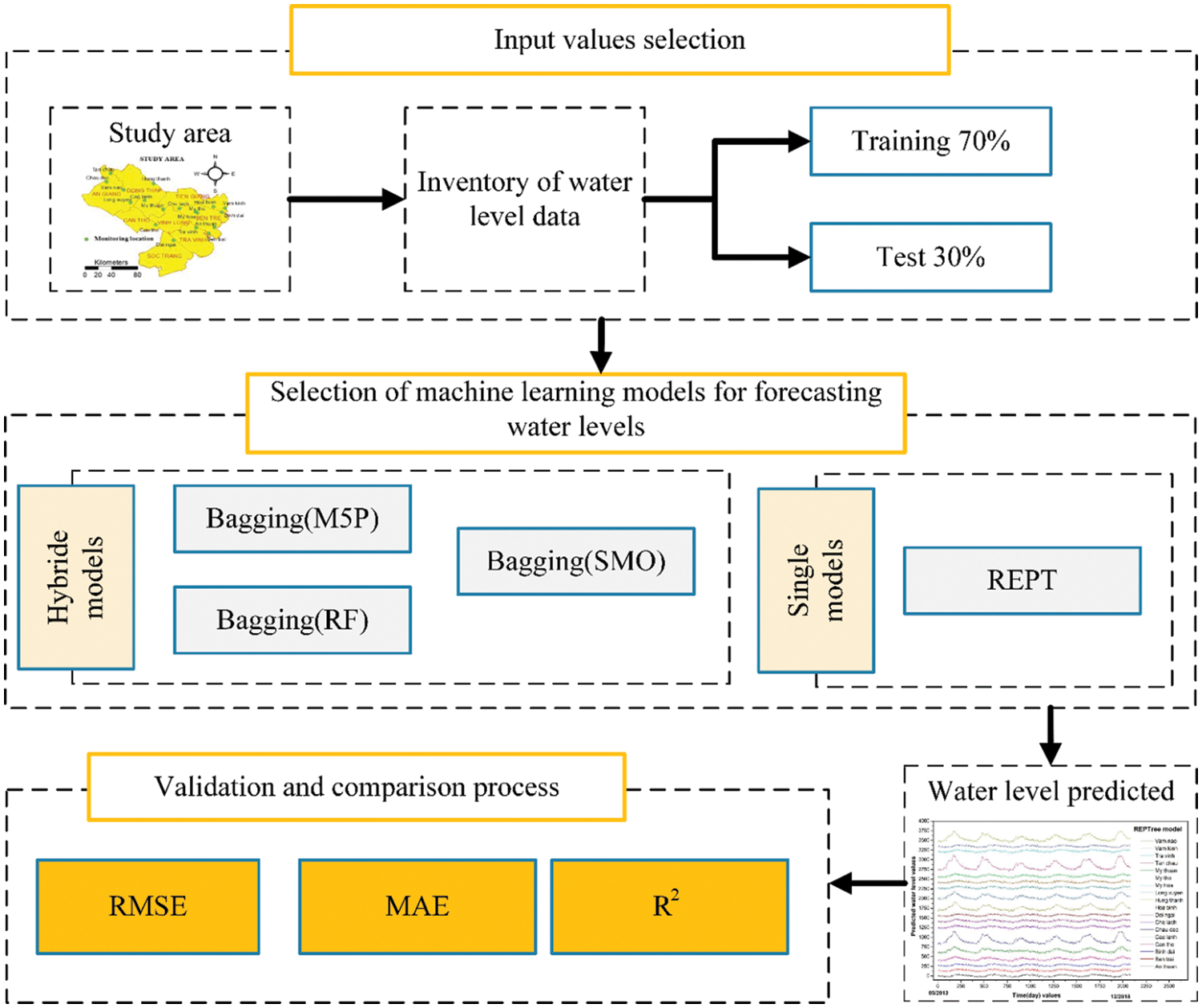
Figure 1: Methodology of water level prediction models
In the Bagging method, a subset of the main data set is given to each of the predictors. That is, each predictor observes a portion of the data set and must build its model based on the same portion of the data provided (i.e., the entire database is not given to each of the predictors) [17]. The Bagging tree stands for Bootstrap aggregating (Bagging) [18,19], which is described in this section. The Bagging algorithm consists of a set of basic models and operates in the following order [20]. Receiving training set D with size N (number of samples of training data), as many as K new training set Di, with size n < N, is produced, which is the result of uniform sampling and replacement of the original set D. As we know, this type of sampling is known as Bootstrap sample. K different models are trained using K subsets and finally form a final model. This final model is obtained in regression by averaging the results of the models and in the classification by voting between the models. The Bagging tree is actually the Bagging algorithm whose basic models are based on decision trees [21].
Input:
Sequence of N examples D < (x1, y1),…, (xN, yN) > with labels yi€ Y = (1,…,L)
Distribution D over the N example
Integer K specifying number of iterations
Weak Learning algorithm Weak Learn (tree)
Do k = 1, 2,…, K
• Choose bootstrapped sample Di (n sample) by randomly from D.
• Call Weak Learn k with Di and receive the hypothesis (tree) ht.
• Add ht to the ensemble.
End
Test: Simple Majority Voting–Given unlabeled instance x
• Evaluate the ensemble (h1,…, hk) on x.
• Choose the class that receives the highest total vote as the final classification.
Among the inputs in the success of cumulative learning methods is the discussion of the diversity of basic models as well as the accuracy of each model. As it is clear, if the basic models are not diverse or so-called diverse, their combination is useless [22]. In the Bagging method, the use of different sets from the original data set guarantees the diversity condition. On the other hand, a model can use changes to its training dataset when it is unstable. Unstable means that small changes in the input (training set) lead to large changes in the output of the model.
RF is a supervised learning algorithm used for both classification and regression [23]. In other words, it is a modern type of tree-based method, which includes a multitude of classification and regression trees. Also, one of the suitable non-parametric methods for modeling continuous and discrete data is the DT method [24]. For example, a forest is made of trees, which means more resilient forest. Similarly, the random tree algorithm makes decision trees on data samples, then predicts each of them, and finally selects the best solution by voting. This is a group method that is better than a single DT, because by averaging the result, it reduces over-fitting [25,26]. Each class is h (x, Φk) for each input instance, where x is an input instance and Φ tutorials are for the k tree. The Φs are independent of each other but with the same distribution. For each sample x, each tree provides a prediction for sample x, and finally the category with the highest number of tree votes on input x is selected as sample. This process is called random forest [27]. RF algorithm can increase the prediction accuracy of individual tree. In the individual tree, instability occurs with small changes in the training set that interfere with the accuracy of the prediction in the experimental sample. But the grouping of a RF algorithm adapts to change and eliminates instability [28]. In general, each tree is formed in 3 ways: (1) If “N” is the number of states in the data set. The “N” mode is randomly sampled by inserting the original data; (2) If there is a variable “M” and “m” is considered smaller than “M”. In each “m” node, the variable is randomly selected from “M” and the best separation on this “m” variable is used to separate the node. That “m” is considered a fixed variable; and (3) Each tree grows as large as possible and there is no pruning [29].
2.1.3 Sequential Minimal Optimization (SMO)
SMO algorithm has the ability to be solved without any additional matrix repository and using numeric optimization sections [30]. In fact, SMO breaks down quadratic programming subjects into quadratic programming subtasks using Osuna’s theory to certify convergence [31,32]. The SMO algorithm is dedicated to selecting α pairs for optimization. There are various methods to select these ingredients to optimize. Hence, there is not “false” method to create this election, howbeit, the order of these options can variate the rate of SMO convergence [33]. In general, the SMO model has two important characteristics: An analytical method for solving the problem of both Lagrange coefficients, and an innovative method for selecting optimization coefficients [34].
where y specifies the target, α is the Lagrange coefficient, and k represents the negative value of the constraints [35].
It should be explained at the outset that the decision tree for constructing predictions creates a tree-like structure in that it first begins its work by using all the instructional samples and selects the variable that performs the best prediction model. Tree branches are the result of a test performed by the algorithm on intermediate nodes at each stage [36]. Predictions also appear on tree leaves [37]. M5P tree model has the ability to predict numerically continuous variables from numerical traits and the predicted results appear as multivariate linear regression models on tree leaves [38]. The criterion of division in a node is based on the selection of the standard deviation of the output values that reach that node as a measure of error. By testing each attribute (parameter) in the node, the expected reduction in error is calculated. The reduction in standard deviation is calculated by Eq. (1) [39]:
where SDR is the standard deviation reduction. T represents the series of instances that reach the node, m is the number of instances that have no missing values for this attribute, β(i) is a correction factor, and TL and TR are sets that result from division on this attribute. Tree pruning means removing extra nodes to prevent the tree from over-fitting into the training data. The final step in building tree models is smoothing to compensate for the inconsistencies that inevitably occur between adjacent linear models in pruned tree leaves [40].
2.1.5 Reduced Error Pruning Trees (REPT)
REPT model consists of two algorithms namely Reduced Error Pruning (REP) and the Decision Tree (DT). In this method, the reason why both REP and DT algorithms are used is that DT is used to facilitate the modeling process using training data when the output of the decision tree is high [41,42]. Also, the reason for using REPT algorithm is reduction of variance and decision tree error. On the other hand, to reduce the variance, the REPT algorithm forms a decision and regression tree using the division standard/criterion [43]. In general, the use of decision trees is a very specific method for classification topics due to its simple structure. Another way to simplify DT is to reduce the use of tree pruning, which can reduce the error due to variance [44]. REPT model after pruning trees is looking for the lowest text and the most accurate subset. The performance of this model is relying on information obtained from decline of variance and diminution of error pruning methods [45]. Therefore, there are two methods for pruning trees before and after pruning. When the instances that reach a node are less than the instructional data, that node is not split. As a result, the generalization error increases. Because the development of the tree stops when the algorithm is constructed, this proceeding is named before pruning [46]. But in the next stage after pruning, all the leaves of the trees develop and increase and there is no error in the educational process. But sub-trees are found for pruning. So, each subset of trees is replaced by a leaf. Because the specimens that are under the tree are trained as soon as a leaf leads to an error, prune the sub-tree and use the leaves. But otherwise, they must be kept under the tree [47].
To evaluate performance of the models used, their accuracy and validity are measured by matching the measured and estimated values of output data [48–50]. Accuracy of the models is estimated based on the training data and for model validation testing data is used [51]. Performance of the models was evaluated using standard statistical criteria such as R2, RMSE and MAE [52,53]. The R2 indicates the probability of correlation between the two data sets. This coefficient actually expresses the approximate results of the desired parameter in the future based on a defined mathematical model that is consistent with the available data [54–56]. The R2 indicates the explanatory power of the model. It indicates what percentage of the changes in the dependent variable are explained by the independent variables [57,58]. A method of estimating the amount of error is the difference between the estimated values and what is estimated. RMSE is almost everywhere positive (not zero) for two reasons: first, because it is random, and second, because the estimator does not count information that can produce more accurate estimates [59]. So, this index, which always has a negative value, the closer it is to zero, the lower the error rate. RMSE includes estimator variance and bias [60,61]. For a non-bias estimator, RMSE is the variance of the estimator [62,63]. Like variance, RMSE has the same units of measurement as squares of estimated values [64,65]. Compared to the standard deviation of the second root from RMSE, presents the root mean square error or the root mean standard deviation (square root mean square error) [66]. Due to various environmental factors commonly known as noise, the measurement operation on each variable may be associated with an error that results in an inaccurate measurement operation. Generally, in the report of precise and formal works, the amount of measurement error is written together with the measured value of the relevant parameter. By reducing the ambient noise, calibrating the instruments used, repeating the test process and measuring the parameters several times, the amount of error can be significantly reduced, but it can never be reduced to zero [67].Therefore, the MAE method is used. The method for estimating the error rate is the average difference between the predicted value and the actual value in all test cases [68,69]. This error is the average prediction error [70]. The formulas of the methods described below are listed as equations [71–73]:
where N is the total number of data, Ksi is the predicted water level data, Koi is the measured water level data,
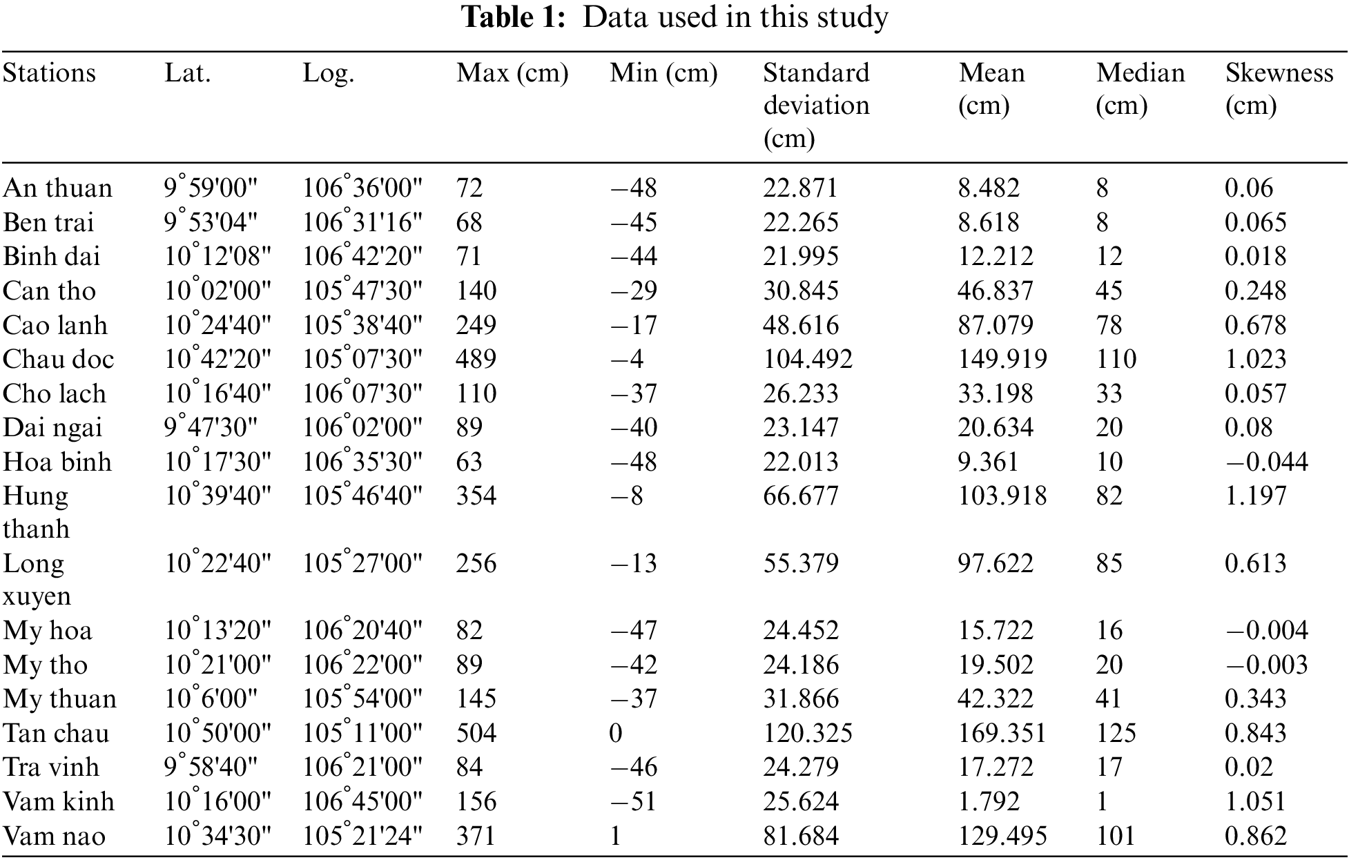
In this study, the data of daily water level was collected from 18 stations located in the Mekong River delta where floods are one of ruinous normal risks in the region, which has an incredible force and potential to hurt characteristic territories and people [74,75]. Water in this delta is descending from the rivers originating from Tibetan plateau and flowing into South Vietnam Sea through distributary channels of Mekong Delta. The study area is a part of the Mekong Delta in the provinces of An Giang, Dong Thap, Can Tho, Tien Giang, Ben Tre, Vinh Long, Tra Vinh and Soc Trang (Vietnam) (Fig. 2). The study area is flat (0–2 m) and covers an area of over 30000 km2. Crops here are mainly wet rice and fruit trees and are currently affected by drought and saltwater intrusion. The Mekong River flow at lower reaches in the delta comes mainly from upstream snow melting and rainfall which fluctuates mainly due to seasonal changes. Water levels in the area are also affected by local rainfall and tides near coast. The climate in this area has two basic seasons: the rainy season from May to September and the dry season from October to March. The average daytime temperature is 32 degrees, at night 24 degree (http://hikersbay.com/climate/vietnam/mekongdelta?lang=vi). The water level in the study area depends mainly on the water volume of the Mekong River Basin. According to monitoring data from 18 water level measurement stations during 19 years, the area fluctuates in typical water level with an annual repeating cycle with the highest water level rising in January and December, the lowest water level in June-July. The land cover changes in the Mekong River basin also cause changes in the runoff pattern and morphology of the area thus impacting water level fluctuation in the study area.
For this study, the surface water level data of the Mekong Delta, Vietnam for 19 years period (01/01/2000–31/12/2018) was used in the modeling. This data was collected from the National Centre for Hydro-Meteorological Forecasting, Vietnam from 18 stations located in 18 tributaries namely An thuan, Ben trai, Binh dai, Can tho, Cao lanh, Chau doc, Cho lach, Dai ngai, Hoa binh, Hung thanh, Long look, My hoa, My tho, My thuan, Tan chau, Tra vinh, Vam kinh, Vam Nao (Fig. 2). Table 1 shows the statistical analysis of the daily water level data. Maximum water level (5.04 m) was recorded at the Tan Chau station whereas the minimum water level (−0.51 m) at the Vam Kinh station. For training the model, data from 1/2000 to 5/2013 was used and for testing/validating the models from 5/2013 to 12/2018 was used, which is about 70% and 30%, respectively, of total water level data. This training/testing ratio (70/30) selected was based on our experience and published literature [76,77]. In this study, we have developed and used the time series models; thus, the date-time (day, month and year) was used as input variables, and the output is the daily water level.
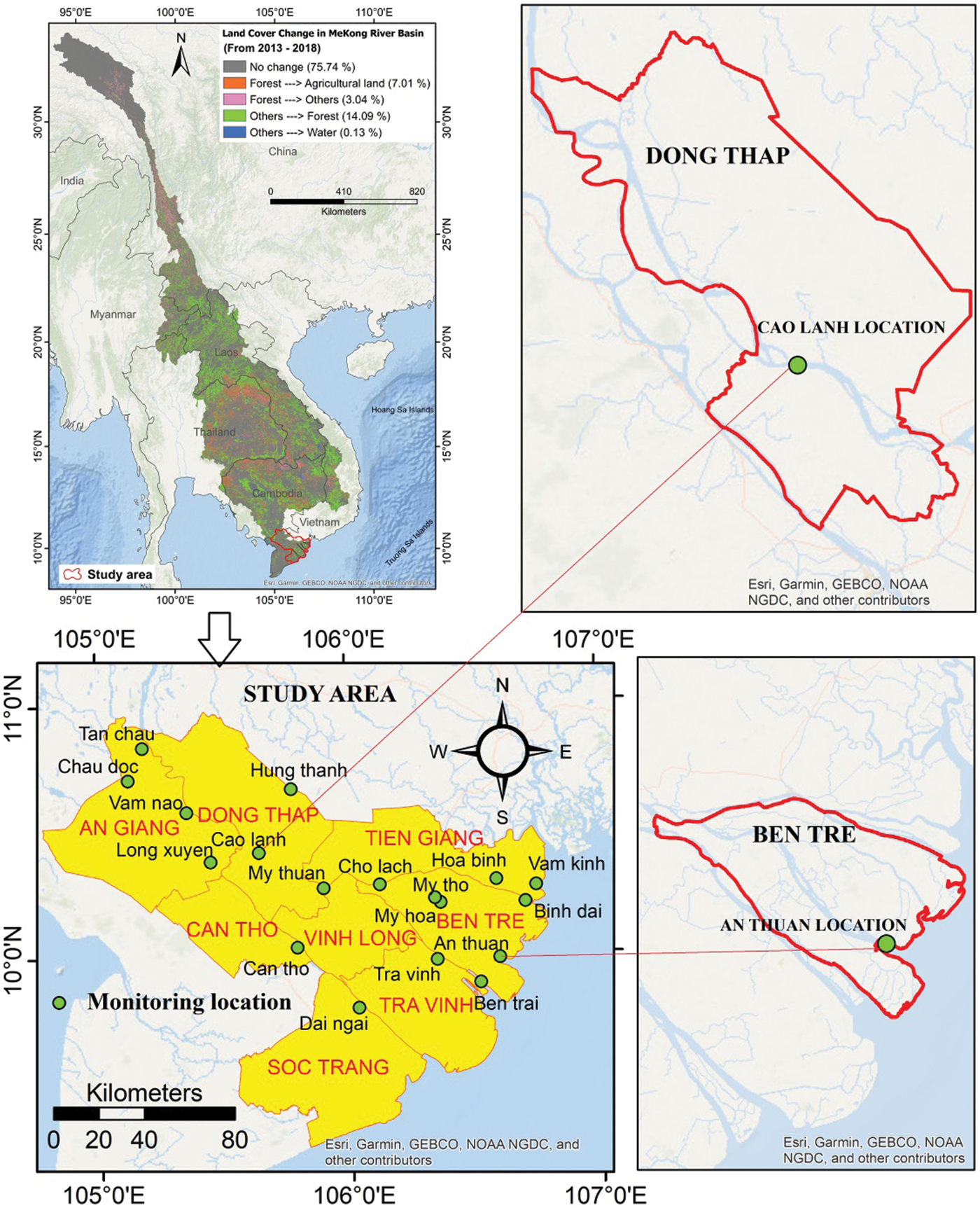
Figure 2: Location of 18 surface water level measurement stations
Validation of the models was done using different statistical indicators namely RMSE, MAE and R2 on both training and testing dataset. While the validation of the models on training dataset indicates the goodness of fit of the models with the data used, on the other hand the validation of the models on testing dataset indicates the predictive capability of the models. In this study, hyper-parameters of each model has been selected by trial-error process to train the models as shown in Table 2. Validation and comparison results of the models are presented in Fig. 3 and Table 3.
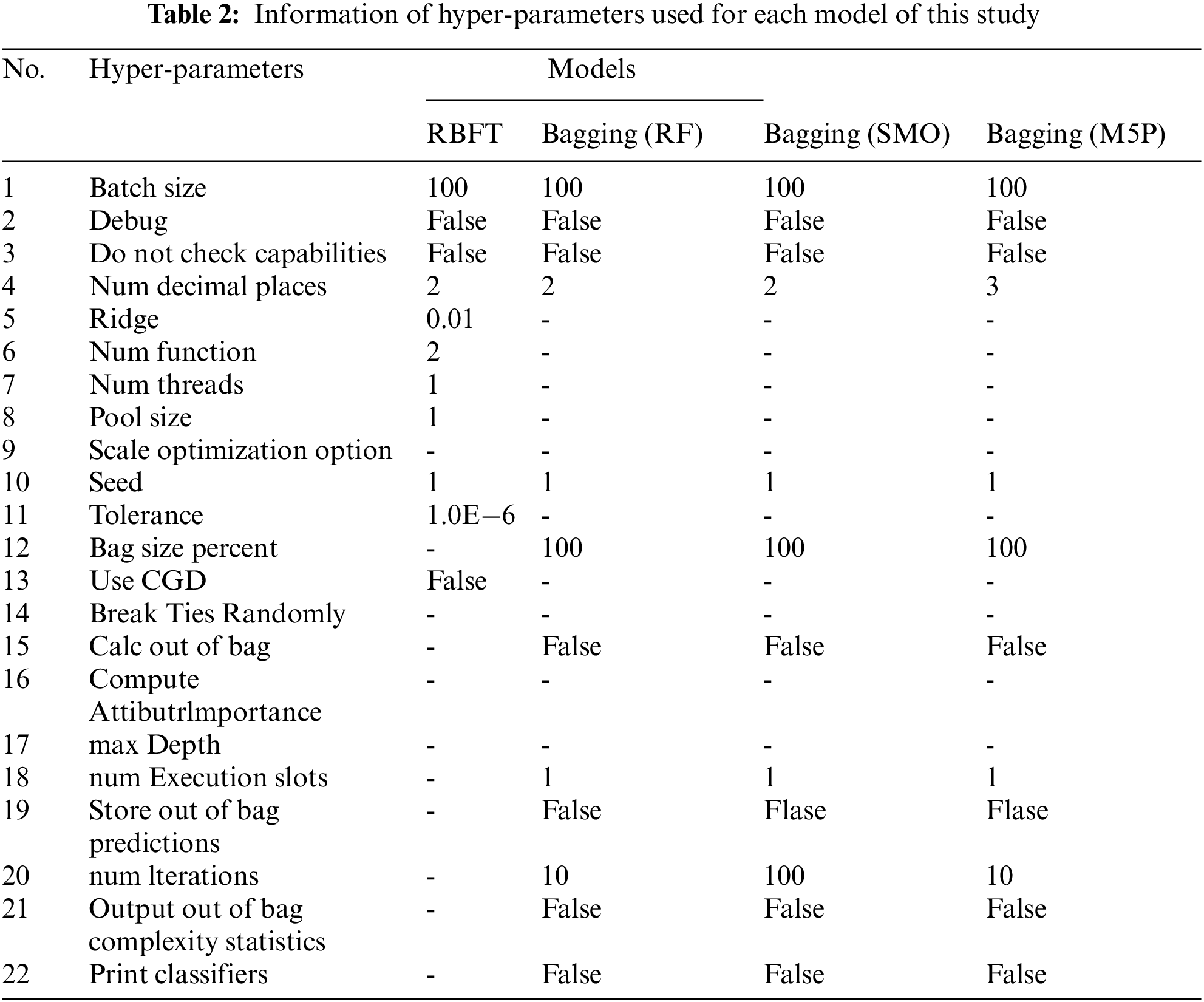
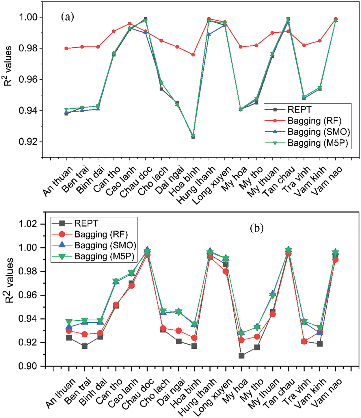
Figure 3: R2 analysis of the models using (a) training and (b) testing datasets
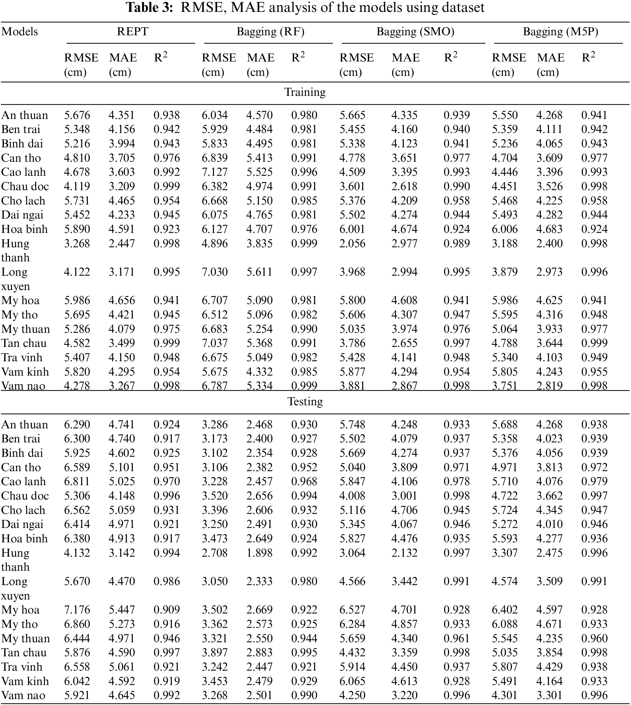
In the case of training dataset (Fig. 3a and Table 3), it can be observed that in the case of REPT model, the R2 values vary from 0.923 to 0.999, the RMSE values differ from 3.268 to 5.986 cm, and the MAE values are from 2.447 to 4.656 cm, for the different stations. With Bagging (RF), the R2 values range from 0.976 to 0.999, the RMSE values differ from 4.896 to 7.127 cm, and the MAE values are from 3.835 to 5.611 cm, for the different stations. Regarding Bagging (SMO), the R2 values differ from 0.924 to 0.998, the RMSE values differ from 2.056 to 6.001 cm, and the MAE values are from 2.618 to 4.674 cm, for the different stations. For Bagging (M5P), the R2 values are from 0.924 to 0.999, the RMSE values differ from 3.118 to 6.006 cm, and the MAE values are from 2.4 to 4.683 cm, for the different stations. From these results, we can see that in all stations, all models have a great goodness of fit with the data used as the R2 values are higher than 0.9 and the RMSE and MAE values are smaller than standard deviation of these indicators (Table 3).
In the case of testing dataset (Fig. 3b and Table 3), it can be seen that the R2 values vary from 0.909 to 0.997, the RMSE values differ from 4.123 to 7.176 cm, and the MAE values are from 3.142 to 5.447 cm, for the different stations in the case of REPT model. For Bagging (RF), the R2 values differ from 0.921 to 0.995, the RMSE values differ from 2.708 to 3.897 cm, and the MAE values are from 1.898 to 2.883 cm, for the different stations. With Bagging (SMO), the R2 values range from 0.928 to 0.998, the RMSE values differ from 3.064 to 6.527 cm, and the MAE values are from 2.132 to 4.857 cm, for the different stations. Regarding Bagging (M5P), the R2 values are from 0.928 to 0.998, the RMSE values differ from 3.307 to 6.402 cm, and the MAE values are from 2.475 to 4.671 cm, for the different stations. Based on these results, it can be seen that all models have good predictive capability for prediction of water level in all stations as R2 values are higher than 0.92 and the RMSE and MAE values are smaller than standard deviation of these indicators (Table 3). As an example, Figs. 4 and 5 shows the actual water level and predicted water level values using different hybrid models at the An Thuan station. Fig. 6 shows the R2 plots of the hybrid models at the An Thuan station.
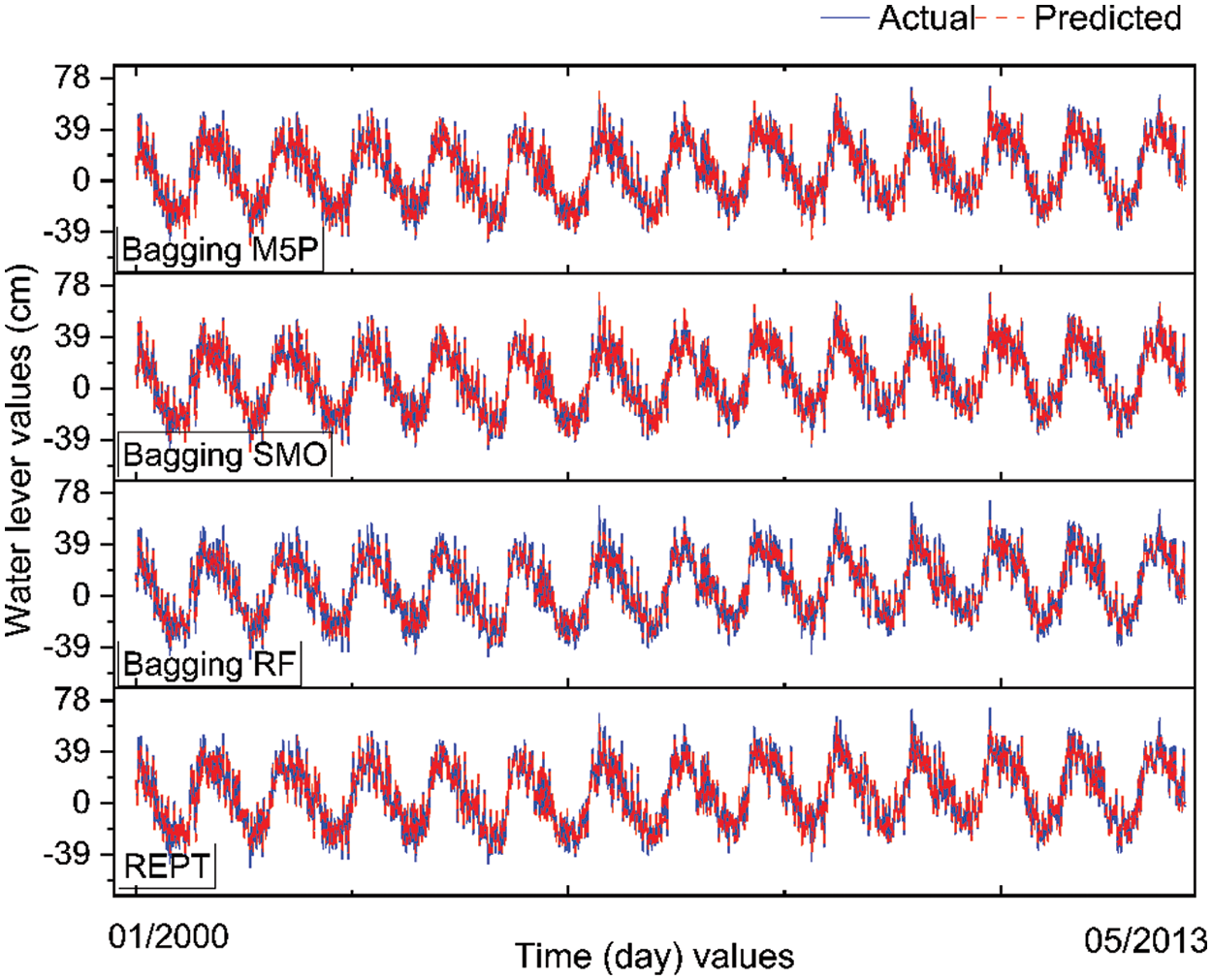
Figure 4: Values of water level predicted from the Bagging (M5P) using training dataset
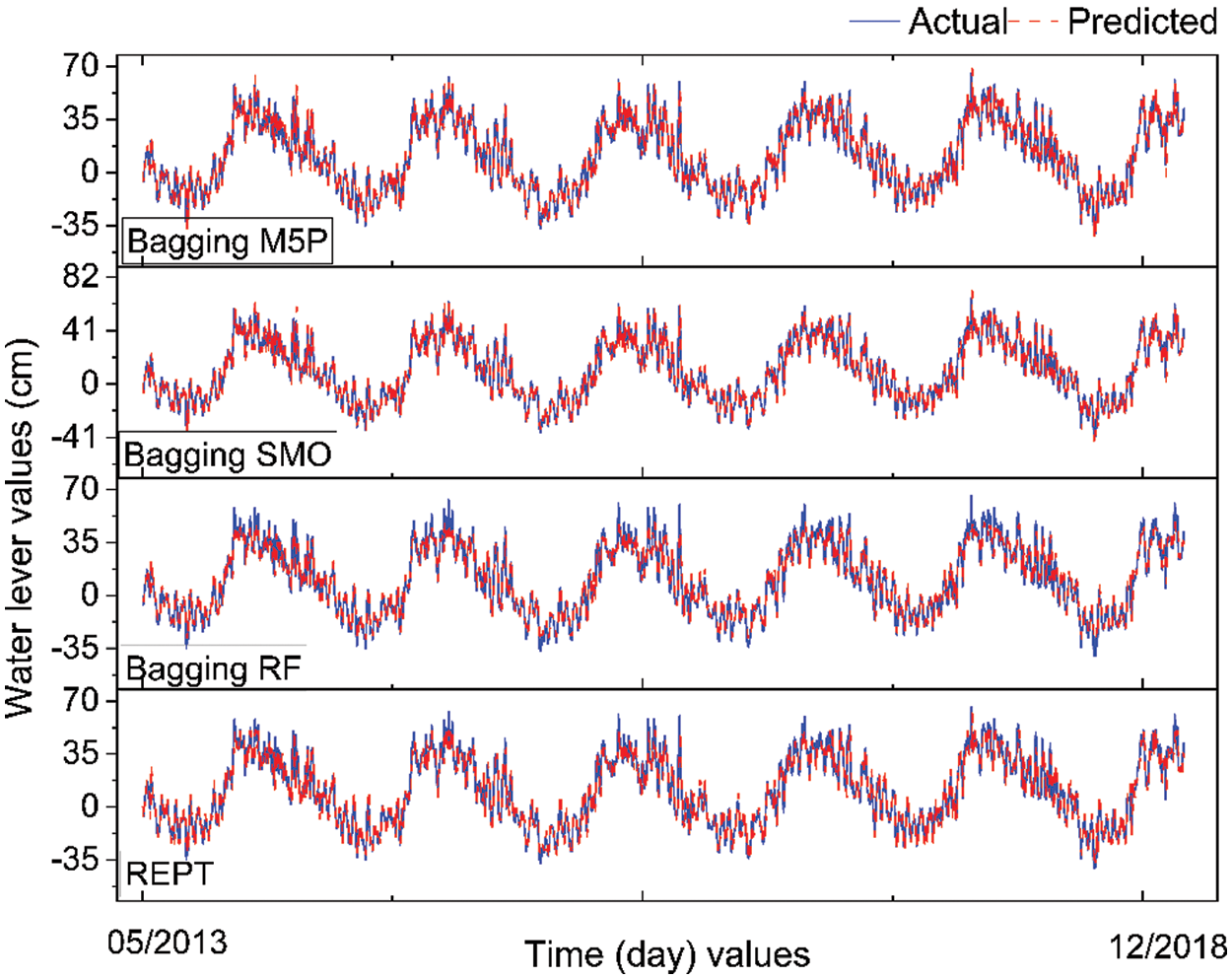
Figure 5: Values of water level predicted from the Bagging (M5P) using testing dataset
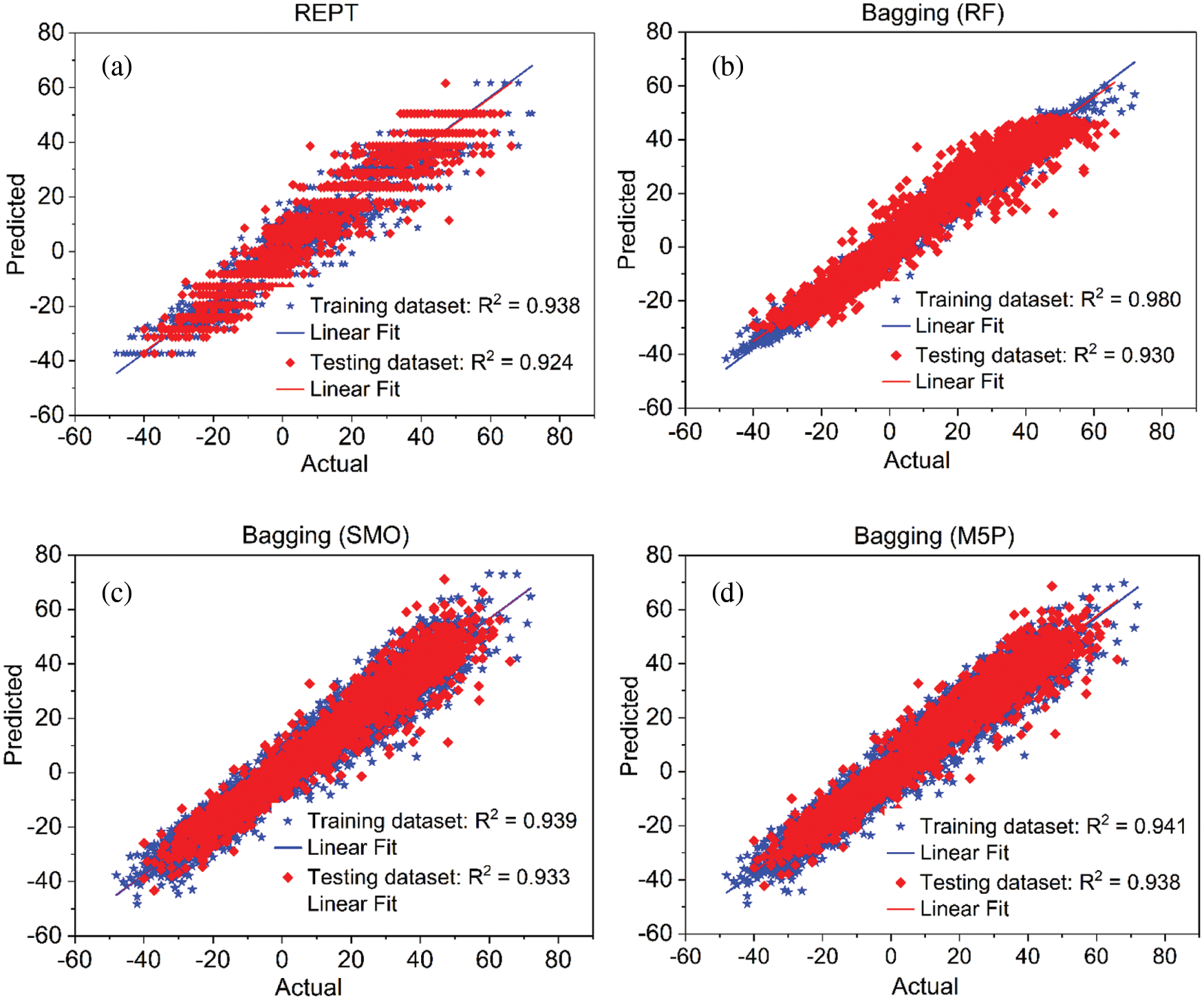
Figure 6: R2 plots of the models at the An Thuan station: (a) REPT, (b) Bagging (RF), (c) Bagging (SMO), and (d) Bagging (M5P)
In general, the performance of all the models developed and used in this study is good for the prediction of water level in the study area. However, it can be observed that performance of the Bagging based hybrid models is slightly better than REPT based on the comparison of the R2, RMSE and MAE values on both training and testing datasets.
Good performance of the Bagging based hybrid models used in this study can be explained that in these hybrid models, the original training dataset was optimized during the training process by using ensemble like Bagging. Optimal training datasets generated were then used in training different classifiers. Finally, a vote is taken among these classifiers, and the class with the highest number of votes is considered the final class for the final classification [78–80]. On the other hand, one of the main advantages of Bagging algorithm is that from among the samples, the mentioned algorithm can select important samples, important samples are samples that increase the diversity in the data set. Using a balanced distribution of weak and hard data, which makes the data set, difficult instances are identified by out-of-bag handlers, so that when a sample is considered “hard” it is incorrectly classified by the ensemble. This hard data is always added to the next data set while easy data has little chance of getting into the dataset [20,81–83]. Performance of the Bagging based hybrid models developed in this study is slightly better than other ML models such as LASSO (R2 = 0.911), Random Forest (R2 = 0.936) and SVM (R2 = 0.935) carried out by Nguyen et al. [13] on Mekong River.
In this study, we have developed and applied novel time-series Bagging-based hybrid models: Bagging (RF), Bagging (SMO), Bagging (M5P), and REPT to predict the daily historical water level data in the southern part of the Mekong delta, Vietnam. In total 4851 surface water level data were collected from the 18 water level measurement stations during 19 years period (1/2000–5/2018) for the models development. Data of 13 years and 5 months period (1/2000–5/2013) was used for training the models and data of 5 years 7 months period for testing the models, which is about 70% and 30% of total data collected during 19 years period. Results indicated that all the studied models performed well in predicting historical water levels but Bagging-based hybrid models are slightly better than another benchmark ML model namely REPT. Thus, Bagging-based hybrid models are promising tools, which can be used for accurate prediction of water levels. These models can also be used for the prediction or forecasting future water levels by adding meteorological data as an input parameter. In this study, local variations due to cyclonic rains have not been considered in the model studies. Model development is continuous process. New hybrid models may continue to be developed considering local geo-environmental and climate change effects for the further improvement in the performance of predictive models.
Data Availability Statement: The data used to support the findings of this study are available from the corresponding author upon request.
Funding Statement: This research was funded by Vietnam Academy of Science and Technology (VAST) under Project Codes KHCBTĐ.02/19-21 and UQĐTCB.02/19-20.
Conflicts of Interest: The authors declare that they have no conflicts of interest to report regarding the present study.
1. Ly, P. T., Thuy, H. L. T. (2019). Spatial distribution of hot days in north central region, Vietnam in the period of 1980–2013. Vietnam Journal of Earth Sciences, 41(1), 36–45. DOI 10.15625/0866-7187/41/1/13544. [Google Scholar] [CrossRef]
2. Hens, L., Thinh, N. A., Hanh, T. H., Cuong, N. S., Lan, T. D. et al. (2018). Sea-level rise and resilience in Vietnam and the Asia-Pacific: A synthesis. Vietnam Journal of Earth Sciences, 40(2), 126–152. DOI 10.15625/0866-7187/40/2/11107. [Google Scholar] [CrossRef]
3. Thao, N. T. P., Linh, T. T., Ha, N. T. T., Vinh, P. Q., Linh, N. T. (2020). Mapping flood inundation areas over the lower part of the con river basin using sentinel 1A imagery. Vietnam Journal of Earth Sciences, 42(3), 288–297. DOI 10.15625/0866-7187/42/3/15453. [Google Scholar] [CrossRef]
4. Zemtsov, V., Vershinin, D., Khromykh, V., Khromykh, O. (2019). Long-term dynamics of maximum flood water levels in the middle course of the Ob River. IOP Conference Series: Earth and Environmental Science, vol. 400, 012004. Salekhard, Russian Federation, IOP Publishing. [Google Scholar]
5. Chen, Y., Gan, M., Pan, S., Pan, H., Zhu, X. et al. (2020). Application of auto-regressive (AR) analysis to improve short-term prediction of water levels in the Yangtze Estuary. Journal of Hydrology, 590, 125386. DOI 10.1016/j.jhydrol.2020.125386. [Google Scholar] [CrossRef]
6. Singh, K. P., Basant, A., Malik, A., Jain, G. (2009). Artificial neural network modeling of the river water quality—A case study. Ecological Modelling, 220(6), 888–895. DOI 10.1016/j.ecolmodel.2009.01.004. [Google Scholar] [CrossRef]
7. Guven, A., Kişi, Ö. (2011). Estimation of suspended sediment yield in natural rivers using machine-coded linear genetic programming. Water Resources Management, 25(2), 691–704. DOI 10.1007/s11269-010-9721-x. [Google Scholar] [CrossRef]
8. Khadr, M., Elshemy, M. (2017). Data-driven modeling for water quality prediction case study: The drains system associated with Manzala Lake, Egypt. Ain Shams Engineering Journal, 8(4), 549–557. DOI 10.1016/j.asej.2016.08.004. [Google Scholar] [CrossRef]
9. Fallah-Mehdipour, E., Haddad, O. B., Mariño, M. A. (2013). Prediction and simulation of monthly groundwater levels by genetic programming. Journal of Hydro-Environment Research, 7(4), 253–260. DOI 10.1016/j.jher.2013.03.005. [Google Scholar] [CrossRef]
10. Karimi, S., Kisi, O., Shiri, J., Makarynskyy, O. (2013). Neuro-fuzzy and neural network techniques for forecasting sea level in Darwin Harbor, Australia. Computers & Geosciences, 52, 50–59. DOI 10.1016/j.cageo.2012.09.015. [Google Scholar] [CrossRef]
11. Yu, P. S., Chen, S. T., Chang, I. F. (2006). Support vector regression for real-time flood stage forecasting. Journal of Hydrology, 328(3), 704–716. DOI 10.1016/j.jhydrol.2006.01.021. [Google Scholar] [CrossRef]
12. Jafari, M. M., Ojaghlou, H., Zare, M., Schumann, G. J. P. (2021). Application of a novel hybrid wavelet-ANFIS/Fuzzy C-means clustering model to predict groundwater fluctuations. Atmosphere, 12(1), 9. DOI 10.3390/atmos12010009. [Google Scholar] [CrossRef]
13. Nguyen, T. T., Huu, Q. N., Li, M. J. (2015). Forecasting time series water levels on Mekong river using machine learning models. 2015 Seventh International Conference on Knowledge and Systems Engineering (KSE), pp. 292–297. Ho Chi Minh City, Vietnam, IEEE. [Google Scholar]
14. Ehteram, M., Ferdowsi, A., Faramarzpour, M., Al-Janabi, A. M. S., Al-Ansari, N. et al. (2021). Hybridization of artificial intelligence models with nature inspired optimization algorithms for lake water level prediction and uncertainty analysis. Alexandria Engineering Journal, 60(2), 2193–2208. DOI 10.1016/j.aej.2020.12.034. [Google Scholar] [CrossRef]
15. Ghorbani, M. A., Deo, R. C., Karimi, V., Yaseen, Z. M., Terzi, O. (2018). Implementation of a hybrid MLP-FFA model for water level prediction of lake Egirdir, Turkey. Stochastic Environmental Research and Risk Assessment, 32(6), 1683–1697. DOI 10.1007/s00477-017-1474-0. [Google Scholar] [CrossRef]
16. Yaseen, Z. M., Naghshara, S., Salih, S. Q., Kim, S., Malik, A. et al. (2020). Lake water level modeling using newly developed hybrid data intelligence model. Theoretical and Applied Climatology, 141, 1285–1300. DOI 10.1007/s00704-020-03263-8. [Google Scholar] [CrossRef]
17. Xia, T., Zhuo, P., Xiao, L., Du, S., Wang, D. et al. (2021). Multi-stage fault diagnosis framework for rolling bearing based on OHF elman AdaBoost-bagging algorithm. Neurocomputing, 433, 237–251. DOI 10.1016/j.neucom.2020.10.003. [Google Scholar] [CrossRef]
18. Wang, S. M., Zhou, J., Li, C. Q., Armaghani, D. J., Li, X. B. et al. (2021). Rockburst prediction in hard rock mines developing bagging and boosting tree-based ensemble techniques. Journal of Central South University, 28(2), 527–542. DOI 10.1007/s11771-021-4619-8. [Google Scholar] [CrossRef]
19. Zhou, J., Qiu, Y., Khandelwal, M., Zhu, S., Zhang, X. (2021). Developing a hybrid model of jaya algorithm-based extreme gradient boosting machine to estimate blast-induced ground vibrations. International Journal of Rock Mechanics and Mining Sciences, 145, 104856. DOI 10.1016/j.ijrmms.2021.104856. [Google Scholar] [CrossRef]
20. Hsiao, Y. W., Tao, C. L., Chuang, E. Y., Lu, T. P. (2020). A risk prediction model of gene signatures in ovarian cancer through bagging of GA-XGBoost models. Journal of Advanced Research, 30, 113–122. DOI 10.1016/j.jare.2020.11.006. [Google Scholar] [CrossRef]
21. Zhang, H., Ishikawa, M. (2007). Bagging using hybrid real-coded genetic algorithm with pruning and its applications to data classification. International Congress Series, 1301, 184–187. DOI 10.1016/j.ics.2006.12.022. [Google Scholar] [CrossRef]
22. Hu, G., Mao, Z., He, D., Yang, F. (2011). Hybrid modeling for the prediction of leaching rate in leaching process based on negative correlation learning bagging ensemble algorithm. Computers & Chemical Engineering, 35(12), 2611–2617. DOI 10.1016/j.compchemeng.2011.02.012. [Google Scholar] [CrossRef]
23. Zhou, J., Asteris, P. G., Armaghani, D. J., Pham, B. T. (2020). Prediction of ground vibration induced by blasting operations through the use of the Bayesian network and random forest models. Soil Dynamics and Earthquake Engineering, 139, 106390. DOI 10.1016/j.soildyn.2020.106390. [Google Scholar] [CrossRef]
24. Chen, Y., Zheng, W., Li, W., Huang, Y. (2021). Large group activity security risk assessment and risk early warning based on random forest algorithm. Pattern Recognition Letters, 144, 1–5. DOI 10.1016/j.patrec.2021.01.008. [Google Scholar] [CrossRef]
25. Simsekler, M. C. E., Qazi, A., Alalami, M. A., Ellahham, S., Ozonoff, A. (2020). Evaluation of patient safety culture using a random forest algorithm. Reliability Engineering & System Safety, 204, 107186. DOI 10.1016/j.ress.2020.107186. [Google Scholar] [CrossRef]
26. Das, S., Chakraborty, R., Maitra, A. (2017). A random forest algorithm for nowcasting of intense precipitation events. Advances in Space Research, 60(6), 1271–1282. DOI 10.1016/j.asr.2017.03.026. [Google Scholar] [CrossRef]
27. Mohana, R. M., Reddy, C. K. K., Anisha, P. R., Murthy, B. V. R. (2021). Random forest algorithms for the classification of tree-based ensemble. Materials Today: Proceedings. DOI 10.1016/j.matpr.2021.01.788. [Google Scholar] [CrossRef]
28. Balachandar, K., Jegadeeshwaran, R. (2021). Friction stir welding tool condition monitoring using vibration signals and random forest algorithm–A machine learning approach. Materials Today: Proceedings, 46, 1174–1180. DOI 10.1016/j.matpr.2021.02.061. [Google Scholar] [CrossRef]
29. Cho, J., Kim, S. (2020). Personal and social predictors of use and non-use of fitness/diet app: Application of Random Forest algorithm. Telematics and Informatics, 55, 101301. DOI 10.1016/j.tele.2019.101301. [Google Scholar] [CrossRef]
30. He, Y., Yuen, S. Y., Lou, Y., Zhang, X. (2019). A sequential algorithm portfolio approach for black box optimization. Swarm and Evolutionary Computation, 44, 559–570. DOI 10.1016/j.swevo.2018.07.001. [Google Scholar] [CrossRef]
31. Chamanbaz, M., Bouffanais, R. (2020). A sequential algorithm for sampled mixed-integer optimization problems. IFAC-PapersOnLine, 53(2), 6749–6755. DOI 10.1016/j.ifacol.2020.12.317. [Google Scholar] [CrossRef]
32. Noronha, D. H., Torquato, M. F., Fernandes, M. A. C. (2019). A parallel implementation of sequential minimal optimization on FPGA. Microprocessors and Microsystems, 69, 138–151. DOI 10.1016/j.micpro.2019.06.007. [Google Scholar] [CrossRef]
33. Yu, J., Shi, Y., Tang, D., Liu, H., Tian, L. (2019). Optimizing sequential diagnostic strategy for large-scale engineering systems using a quantum-inspired genetic algorithm: A comparative study. Applied Soft Computing, 85, 105802. DOI 10.1016/j.asoc.2019.105802. [Google Scholar] [CrossRef]
34. Papadrakakis, M., Lagaros, N. D., Tsompanakis, Y. (1998). Structural optimization using evolution strategies and neural networks. Computer Methods in Applied Mechanics and Engineering, 156(1), 309–333. DOI 10.1016/S0045-7825(97)00215-6. [Google Scholar] [CrossRef]
35. Lhomme, O., Gotlieb, A., Rueher, M. (1998). Dynamic optimization of interval narrowing algorithms. The Journal of Logic Programming, 37(1), 165–183. DOI 10.1016/S0743-1066(98)10007-9. [Google Scholar] [CrossRef]
36. Behnood, A., Daneshvar, D. (2020). A machine learning study of the dynamic modulus of asphalt concretes: An application of M5P model tree algorithm. Construction and Building Materials, 262, 120544. DOI 10.1016/j.conbuildmat.2020.120544. [Google Scholar] [CrossRef]
37. Behnood, A., Behnood, V., Modiri Gharehveran, M., Alyamac, K. E. (2017). Prediction of the compressive strength of normal and high-performance concretes using M5P model tree algorithm. Construction and Building Materials, 142, 199–207. DOI 10.1016/j.conbuildmat.2017.03.061. [Google Scholar] [CrossRef]
38. Akgündoğdu, A., Öz, I., Uzunoğlu, C. P. (2019). Signal quality based power output prediction of a real distribution transformer station using M5P model tree. Electric Power Systems Research, 177, 106003. DOI 10.1016/j.epsr.2019.106003. [Google Scholar] [CrossRef]
39. Balouchi, B., Nikoo, M. R., Adamowski, J. (2015). Development of expert systems for the prediction of scour depth under live-bed conditions at river confluences: Application of different types of ANNs and the M5P model tree. Applied Soft Computing, 34, 51–59. DOI 10.1016/j.asoc.2015.04.040. [Google Scholar] [CrossRef]
40. Dang, S. K., Singh, K. (2021). Predicting tensile-shear strength of nugget using M5P model tree and random forest: An analysis. Computers in Industry, 124, 103345. DOI 10.1016/j.compind.2020.103345. [Google Scholar] [CrossRef]
41. Dai, Q., Zhang, T., Liu, N. (2015). A new reverse reduce-error ensemble pruning algorithm. Applied Soft Computing, 28, 237–249. DOI 10.1016/j.asoc.2014.10.045. [Google Scholar] [CrossRef]
42. Onan, A., Korukoğlu, S., Bulut, H. (2017). A hybrid ensemble pruning approach based on consensus clustering and multi-objective evolutionary algorithm for sentiment classification. Information Processing & Management, 53(4), 814–833. DOI 10.1016/j.ipm.2017.02.008. [Google Scholar] [CrossRef]
43. Kim, J., Kim, Y. (2006). Maximum a posteriori pruning on decision trees and its application to bootstrap BUMPing. Computational Statistics & Data Analysis, 50(3), 710–719. DOI 10.1016/j.csda.2004.09.010. [Google Scholar] [CrossRef]
44. Kappelhof, N., Ramos, L. A., Kappelhof, M., van Os, H. J. A., Chalos, V. et al. (2021). Evolutionary algorithms and decision trees for predicting poor outcome after endovascular treatment for acute ischemic stroke. Computers in Biology and Medicine, 133, 104414. DOI 10.1016/j.compbiomed.2021.104414. [Google Scholar] [CrossRef]
45. Karkee, M., Adhikari, B., Amatya, S., Zhang, Q. (2014). Identification of pruning branches in tall spindle apple trees for automated pruning. Computers and Electronics in Agriculture, 103, 127–135. DOI 10.1016/j.compag.2014.02.013. [Google Scholar] [CrossRef]
46. Mirmahaleh, S. Y. H., Rahmani, A. M. (2019). DNN pruning and mapping on NoC-based communication infrastructure. Microelectronics Journal, 94, 104655. DOI 10.1016/j.mejo.2019.104655. [Google Scholar] [CrossRef]
47. Pham, B. T., Prakash, I., Singh, S. K., Shirzadi, A., Shahabi, H. et al. (2019). Landslide susceptibility modeling using reduced error pruning trees and different ensemble techniques: Hybrid machine learning approaches. CATENA, 175, 203–218. DOI 10.1016/j.catena.2018.12.018. [Google Scholar] [CrossRef]
48. Mohammed, A. S., Asteris, P. G., Koopialipoor, M., Alexakis, D. E., Lemonis, M. E. et al. (2021). Stacking ensemble tree models to predict energy performance in residential buildings. Sustainability, 13(15), 8298. DOI 10.3390/su13158298. [Google Scholar] [CrossRef]
49. Asteris, P. G., Koopialipoor, M., Armaghani, D. J., Kotsonis, E. A., Lourenço, P. B. (2021). Prediction of cement-based mortars compressive strength using machine learning techniques. Neural Computing and Applications, 33, 1–33. DOI 10.1007/s00521-021-06004-8. [Google Scholar] [CrossRef]
50. Tang, D., Gordan, B., Koopialipoor, M., Jahed Armaghani, D., Tarinejad, R. et al. (2020). Seepage analysis in short embankments using developing a metaheuristic method based on governing equations. Applied Sciences, 10(5), 1761. DOI 10.3390/app10051761. [Google Scholar] [CrossRef]
51. de Bondt, G. J., Hahn, E., Zekaite, Z. (2021). ALICE: Composite leading indicators for euro area inflation cycles. International Journal of Forecasting, 37(2), 687–707. DOI 10.1016/j.ijforecast.2020.09.001. [Google Scholar] [CrossRef]
52. Jahed Armaghani, D., Asteris, P. G., Askarian, B., Hasanipanah, M., Tarinejad, R. et al. (2020). Examining hybrid and single SVM models with different kernels to predict rock brittleness. Sustainability, 12(6), 2229. DOI 10.3390/su12062229. [Google Scholar] [CrossRef]
53. Hajihassani, M., Abdullah, S. S., Asteris, P. G., Armaghani, D. J. (2019). A gene expression programming model for predicting tunnel convergence. Applied Sciences, 9(21), 4650. DOI 10.3390/app9214650. [Google Scholar] [CrossRef]
54. Hong, T., Kim, C. J., Jeong, J., Kim, J., Koo, C. et al. (2016). Framework for approaching the minimum CV(RMSE) using energy simulation and optimization tool. Energy Procedia, 88, 265–270. DOI 10.1016/j.egypro.2016.06.157. [Google Scholar] [CrossRef]
55. Pham, B. T., Nguyen, M. D., Nguyen-Thoi, T., Ho, L. S., Koopialipoor, M. et al. (2021). A novel approach for classification of soils based on laboratory tests using adaboost, tree and ANN modeling. Transportation Geotechnics, 27, 100508. DOI 10.1016/j.trgeo.2020.100508. [Google Scholar] [CrossRef]
56. Cai, M., Koopialipoor, M., Armaghani, D. J., Thai Pham, B. (2020). Evaluating slope deformation of earth dams due to earthquake shaking using MARS and GMDH techniques. Applied Sciences, 10(4), 1486. DOI 10.3390/app10041486. [Google Scholar] [CrossRef]
57. Polášek, M., Kohoutková, D., Waisser, K. (1988). Kinetic spectrophotometric determination of thiobenzamides and their partition coefficients in water/1-octanol by using an iodine/azide indicator reaction. Analytica Chimica Acta, 212, 279–284. DOI 10.1016/S0003-2670(00)84151-3. [Google Scholar] [CrossRef]
58. Vogler, N., Lindemann, M., Drabetzki, P., Kühne, H. C. (2020). Alternative pH-indicators for determination of carbonation depth on cement-based concretes. Cement and Concrete Composites, 109, 103565. DOI 10.1016/j.cemconcomp.2020.103565. [Google Scholar] [CrossRef]
59. Huang, L., Asteris, P. G., Koopialipoor, M., Armaghani, D. J., Tahir, M. (2019). Invasive weed optimization technique-based ANN to the prediction of rock tensile strength. Applied Sciences, 9(24), 5372. DOI 10.3390/app9245372. [Google Scholar] [CrossRef]
60. Liemohn, M. W., Shane, A. D., Azari, A. R., Petersen, A. K., Swiger, B. M. et al. (2021). RMSE is not enough: Guidelines to robust data-model comparisons for magnetospheric physics. Journal of Atmospheric and Solar-Terrestrial Physics, 218, 105624. DOI 10.1016/j.jastp.2021.105624. [Google Scholar] [CrossRef]
61. Armaghani, D. J., Asteris, P. G. (2021). A comparative study of ANN and ANFIS models for the prediction of cement-based mortar materials compressive strength. Neural Computing and Applications, 33(9), 4501–4532. DOI 10.1007/s00521-020-05244-4. [Google Scholar] [CrossRef]
62. Asteris, P. G., Lemonis, M. E., Nguyen, T. A., van Le, H., Pham, B. T. (2021). Soft computing-based estimation of ultimate axial load of rectangular concrete-filled steel tubes. Steel and Composite Structures, 39(4), 471. DOI 10.12989/scs.2021.39.4.471. [Google Scholar] [CrossRef]
63. Asteris, P. G., Cavaleri, L., Ly, H. B., Pham, B. T. (2021). Surrogate models for the compressive strength mapping of cement mortar materials. Soft Computing, 25(8), 6347–6372. DOI 10.1007/s00500-021-05626-3. [Google Scholar] [CrossRef]
64. Ly, H. B., Pham, B. T., Le, L. M., Le, T. T., Le, V. M. et al. (2021). Estimation of axial load-carrying capacity of concrete-filled steel tubes using surrogate models. Neural Computing and Applications, 33(8), 3437–3458. DOI 10.1007/s00521-020-05214-w. [Google Scholar] [CrossRef]
65. Duan, J., Asteris, P. G., Nguyen, H., Bui, X. N., Moayedi, H. (2020). A novel artificial intelligence technique to predict compressive strength of recycled aggregate concrete using ICA-XGBoost model. Engineering with Computers, 37, 1–18. DOI 10.1007/s00366-020-01003-0. [Google Scholar] [CrossRef]
66. Chandola, D., Gupta, H., Tikkiwal, V. A., Bohra, M. K. (2020). Multi-step ahead forecasting of global solar radiation for arid zones using deep learning. Procedia Computer Science, 167, 626–635. DOI 10.1016/j.procs.2020.03.329. [Google Scholar] [CrossRef]
67. Fan, J., Zheng, J., Wu, L., Zhang, F. (2021). Estimation of daily maize transpiration using support vector machines, extreme gradient boosting, artificial and deep neural networks models. Agricultural Water Management, 245, 106547. DOI 10.1016/j.agwat.2020.106547. [Google Scholar] [CrossRef]
68. Asteris, P. G., Skentou, A. D., Bardhan, A., Samui, P., Lourenço, P. B. (2021). Soft computing techniques for the prediction of concrete compressive strength using non-destructive tests. Construction and Building Materials, 303, 124450. DOI 10.1016/j.conbuildmat.2021.124450. [Google Scholar] [CrossRef]
69. Asteris, P. G., Skentou, A. D., Bardhan, A., Samui, P., Pilakoutas, K. (2021). Predicting concrete compressive strength using hybrid ensembling of surrogate machine learning models. Cement and Concrete Research, 145, 106449. DOI 10.1016/j.cemconres.2021.106449. [Google Scholar] [CrossRef]
70. Hao, X., Qiu, Y., Fan, Y., Li, T., Leng, D. et al. (2020). Applicability of temporal stability analysis in predicting field mean of soil moisture in multiple soil depths and different seasons in an irrigated vineyard. Journal of Hydrology, 588, 125059. DOI 10.1016/j.jhydrol.2020.125059. [Google Scholar] [CrossRef]
71. Nguyen, M. D., Pham, B. T., Ho, L. S., Ly, H. B., Le, T. T. et al. (2020). Soft-computing techniques for prediction of soils consolidation coefficient. CATENA, 195, 104802. DOI 10.1016/j.catena.2020.104802. [Google Scholar] [CrossRef]
72. Chen, J., Li, A., Bao, C., Dai, Y., Liu, M. et al. (2021). A deep learning forecasting method for frost heave deformation of high-speed railway subgrade. Cold Regions Science and Technology, 185, 103265. DOI 10.1016/j.coldregions.2021.103265. [Google Scholar] [CrossRef]
73. Le, T. T., Asteris, P. G., Lemonis, M. E. (2021). Prediction of axial load capacity of rectangular concrete-filled steel tube columns using machine learning techniques. Engineering with Computers, 1–34. DOI 10.1007/s00366-021-01461-0. [Google Scholar] [CrossRef]
74. Thai, T. H., Tri, D. Q. (2019). Combination of hydrologic and hydraulic modeling on flood and inundation warning: Case study at Tra Khuc-Ve River basin in Vietnam. Vietnam Journal of Earth Sciences, 41(3), 240–251. DOI 10.15625/0866-7187/41/3/13866. [Google Scholar] [CrossRef]
75. Van, N. K., Oanh, H. T. K., Van Vu, V. (2019). The bioclimatic map of southern Vietnam for tourism development. Vietnam Journal of Earth Sciences, 41(2), 116–129. DOI 10.15625/0866-7187/41/2/13692. [Google Scholar] [CrossRef]
76. Nguyen, Q. H., Ly, H. B., Ho, L. S., Al-Ansari, N., Le, H. V. et al. (2021). Influence of data splitting on performance of machine learning models in prediction of shear strength of soil. Mathematical Problems in Engineering, 2021, 1–15. DOI 10.1155/2021/4832864. [Google Scholar] [CrossRef]
77. Anifowose, F., Khoukhi, A., Abdulraheem, A. (2017). Investigating the effect of training–testing data stratification on the performance of soft computing techniques: An experimental study. Journal of Experimental & Theoretical Artificial Intelligence, 29(3), 517–535. DOI 10.1080/0952813X.2016.1198936. [Google Scholar] [CrossRef]
78. Tang, X., Gu, X., Rao, L., Lu, J. (2021). A single fault detection method of gearbox based on random forest hybrid classifier and improved dempster-shafer information fusion. Computers & Electrical Engineering, 92, 107101. DOI 10.1016/j.compeleceng.2021.107101. [Google Scholar] [CrossRef]
79. Asadi, S., Roshan, S. E. (2021). A bi-objective optimization method to produce a near-optimal number of classifiers and increase diversity in bagging. Knowledge-Based Systems, 213, 106656. DOI 10.1016/j.knosys.2020.106656. [Google Scholar] [CrossRef]
80. Ji, X., Ren, Y., Tang, H., Xiang, J. (2021). DSmT-based three-layer method using multi-classifier to detect faults in hydraulic systems. Mechanical Systems and Signal Processing, 153, 107513. DOI 10.1016/j.ymssp.2020.107513. [Google Scholar] [CrossRef]
81. Shigei, N., Miyajima, H., Maeda, M., Ma, L. (2009). Bagging and AdaBoost algorithms for vector quantization. Neurocomputing, 73(1), 106–114. DOI 10.1016/j.neucom.2009.02.020. [Google Scholar] [CrossRef]
82. Weber, V. A. M., Weber, F. D. L., Oliveira, A. D. S., Astolfi, G., Menezes, G. V. et al. (2020). Cattle weight estimation using active contour models and regression trees bagging. Computers and Electronics in Agriculture, 179, 105804. DOI 10.1016/j.compag.2020.105804. [Google Scholar] [CrossRef]
83. Menaga, S., Paruvathavardhini, J., Pragaspathy, S., Dhanapal, R., Jebakumar Immanuel, D. (2021). An efficient biometric based authenticated geographic opportunistic routing for IoT applications using secure wireless sensor network. Materials Today: Proceedings. DOI 10.1016/j.matpr.2021.01.241. [Google Scholar] [CrossRef]
 | This work is licensed under a Creative Commons Attribution 4.0 International License, which permits unrestricted use, distribution, and reproduction in any medium, provided the original work is properly cited. |