| Computer Modeling in Engineering & Sciences |
DOI: 10.32604/cmes.2022.019424
ARTICLE
Fluid Analysis and Structure Optimization of Impeller Based on Surrogate Model
School of Mechanical and Electrical Engineering, University of Electronic Science and Technology of China, Chengdu, 611731, China
*Corresponding Author: Huanwei Xu. Email: hwxu@uestc.edu.cn
Received: 23 September 2021; Accepted: 08 December 2021
Abstract: The surrogate model technology has a good performance in solving black-box optimization problems, which is widely used in multi-domain engineering optimization problems. The adaptive surrogate model is the mainstream research direction of surrogate model technology, which can realize model fitting and global optimization of engineering problems by infilling criteria. Based on the idea of the adaptive surrogate model, this paper proposes an efficient global optimization algorithm based on the local remodeling method (EGO-LR), which aims at improving the accuracy and optimization efficiency of the model. The proposed algorithm firstly constructs the expectation improvement (EI) function in the local area and optimizes it to get the update points. Secondly, the obtained update points are added to the global region until the global accuracy of the model meets the requirements. Then the differential evolution algorithm is used for global optimization. Sixteen benchmark functions are used to compare the EGO-LR algorithm with the existing algorithms. The results show that the EGO-LR algorithm can quickly converge to the accuracy requirements of the model and find the optimal value efficiently when facing complex problems with many local extrema and large variable spaces. The proposed algorithm is applied to the optimization design of the structural parameter of the impeller, and the outflow field analysis of the impeller is realized through finite element analysis. The optimization with the maximum fluid pressure (MP value) of the impeller as the objective function is completed, which effectively reduces the pressure value of the impeller under load.
Keywords: The surrogate model; EGO; adaptive; fluid analysis; impeller
The adaptive surrogate model [1] technology can significantly reduce the number of simulations by selecting a small number of experimental points and accelerate the convergence to the global optimal solution when dealing with complex simulation models. The initial experimental design method, model construction, and accurate prediction are the three necessary steps of traditional surrogate model construction. The adaptive surrogate model adds a feedback link in the traditional construction process. In feedback link of the adaptive process,new experimental points are selected and added to the initial sample library through multiple iterations. Generally, the construction of the adaptive surrogate model is closely combined with the global optimization process, the model construction and optimization are carried out at the same time. The EI criterion [2] as a classical adaptive infilling criterion, which is based on the Kriging surrogate model [3] and combined with the prediction error of experimental points to construct the EI function. As an efficient global optimization strategy [4,5], although the EI criterion takes into account the globality and efficiency of optimization, only one update point is generated in each iteration, which means that more iterations are needed to reach the convergence criteria. Therefore, the parallel optimization methods of selecting multiple update points each iteration have become the mainstream research direction of adaptive surrogate model optimization in recent years. There are three main research ideas for parallel optimization: 1) Obtain multiple update points by optimizing the same infilling criterion many times or calculating multiple expectation points of the same criterion; 2) Obtain multiple update points by using different surrogate models or different infilling criteria; 3) Obtain multiple update points by taking multiple infilling criteria as optimization objectives at the same time. The multi-point infilling criteria attempt to make the selected new experimental points have both local search and global search functions. Zhan et al. [6] proposed a pseudo expectation improvement criterion (PEI) of parallel computing multiple update points. The criterion approximates the real updated EI function by multiplying the initial EI function and the influence function (IF) of the update point. Therefore, it can be used without reshaping the expensive function to select multiple candidate points in each iteration, and a new parallel EGO algorithm is proposed based on the PEI criterion. Jian et al. [7] applied the PEI function to find the multi-peak position of the EI function and proposed a multi-point criterion PEI-R, which can achieve the accurate global solution of the optimization problem by obtaining multiple local sampling points. The proposed method has good performance in structural optimization. Ivo et al. [8] applied the probability of improvement (POI) and EI criteria of the Kriging model to multi-objective optimization to identify the Pareto frontier with the least number of expensive simulations. In order to solve the poor performance of the EGO algorithm in high-dimensional optimization problems, Mohamed et al. [9] proposed a “locating the regional extreme” criterion, which includes minimizing the alternative model and maximizing the expected improvement criterion at the same time. According to the quantity and probability of target improvement, Chaudhuri et al. [10] proposed the EGO-AT algorithm. The algorithm adjusts the target in each iteration according to whether the target is achieved in the previous iteration.
The improved global optimization algorithm performs well in numerical optimization problems and can accurately find the optimal value of function in complex mathematical examples [11–13]. At the same time, many scholars apply the global optimization algorithm based on the surrogate model to engineering problems such as fluid analysis and have been effectively verified, which provides an effective method for the field of engineering optimization [14–16]. Yi et al. [17] establishes two surrogate models of spray angle and liquid film thickness based on Kriging's global optimization algorithm, and carry out multi-objective parameter optimization for the swirl nozzle of aero-engine at low-pressure start-up stage. Heo et al. [18] optimized the inlet angle of the expander blade of the mixed-flow pump by using the surrogate model, which greatly improved the efficiency of the mixed-flow pump at the specified speed. Lai et al. [19] optimized the impeller structure with the goal of weight reduction and used a genetic algorithm to globally optimize the Kriging model in the design space, which not only improved the optimization efficiency but also obtained good optimization results. Wang et al. [20] applied Kriging global optimization algorithm to the aerodynamic performance optimization of wind turbine blades. Compared with the numerical simulation method, the obtained aerodynamic efficiency optimization coefficient of blades is higher, but it lacks the improvement of traditional global optimization algorithm, and its optimization process is easy to fall into local search.
Global optimization is closely related to the adaptive surrogate model, and scholars have more extensive research on parallel optimization methods, but the optimization problem still faces difficulties: 1) The number of initial sample points is difficult to determine in the stage of experimental design, which is prone to clustering and degradation in the face of high-dimensional and large sample problems; 2) Too many dimensions and too much variable space will lead to modeling failure or solving difficulty; 3) In the face of high nonlinearity and multiple local extremums, the inaccurate model fitting leads to the death cycle of local search. Given the difficulty of model optimization caused by the large range of design space and many local extrema, this paper proposes an efficient global optimization algorithm based on local remodeling (EGO-LR), which not only balances the local and global search but also speeds up the efficiency of local fitting and global optimization under the condition of ensuring the accuracy.
The remaining chapters of the paper are as follows: In Section 2, the specific construction process of EGO-LR algorithm is proposed in detail. Compared with PEI algorithm, the advantages of EGO-LR algorithm are analyzed; In Section 3, the parametric design of the main structure of the impeller is carried out, and the model is preprocessed in ANSYS CFX; In Section 4, the mathematical model of impeller hydrodynamic analysis is established. Combined with finite element simulation analysis, the EGO-LR algorithm is used to minimize the maximum pressure (MP) of the impeller structure; finally, the EGO-LR algorithm and optimization results are summarized.
2 Global Optimization of Surrogate Model Based on Reshaped Domain
In summarizing scholars' research on the global optimization algorithm, it is found that when the EGO algorithm performs a global search on a large spatial region, the value of the EI function decreases sharply near the update point. In other words, the impact of the update point on the EI function at a certain point depends on the distance between the point and the update point. The smaller the distance, the greater the impact. When the distance is too large, the expectation of the EI function is very low. Therefore, the iterative process has a strong dependence on the previous update point. If the update point is in a wide area, the EGO method gradually carries out a random search in the later stage of optimization, and the convergence degree is slow. Therefore, in the remodeling domain, only one iteration is carried out to search for new sample points, which not only ensures the directionality and expectation of the EGO algorithm search but also avoids the slow search caused by falling into the local optimization.
2.1 The Construction of the EGO-LR Algorithm
The main goal of optimization is to obtain global optimal value which can also be regarded as the minimum extreme value among the local extreme values. Based on the idea of balancing local and global optimization, in order to find an accurate solution and speed up the efficiency of jumping out of local search, the EGO-LR algorithm is constructed with the Kriging. The Kriging model is composed of regression part and nonparametric part. The nonparametric part contains the approximation error of local simulation that has the statistical characteristics of correlation. The correlation of samples is affected by the correlation function. In this paper, we choose the widely used Gaussian correlation function which has the best calculation effect in general. The superparameter θ of Gaussian function affect the correlation of samples and the fitting accuracy of response values. A low value of θ will cause a high correlation between adjacent sample points. A high value of θ will cause the value of the correlation function change too quickly between two points. After consulting a large number of literature and practical examples, in order to make the approximate function have good “activity” when fitting the function response value with higher dimension, and ensure that the test examples in the paper have better contrast under the same parameter conditions, the value of the superparameter θ is an appropriate fixed value 1. Firstly, the EGO-LR algorithm is described in detail based on numerical examples. The specific construction block diagram is shown in Fig. 1.
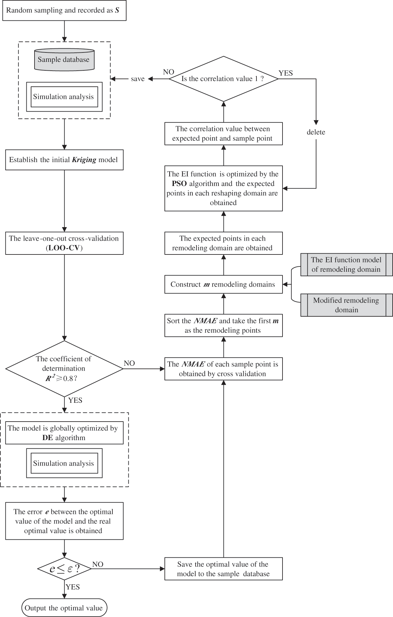
Figure 1: Construction block diagram of the EGO-LR algorithm
The main steps of the EGO-LR algorithm are as follows:
(1) Initial random sampling. The sample distribution formed by the Sobol sequence method [21] is more uniform in high-dimensional space and more conducive to the execution of the algorithm program. In this paper, the Sobol sequence method is used to obtain the initial sample points to improve the balance of sample distribution. The number of sample points is a multiple of N, and N represents the number of dimensions.
(2) Calculate the response value of each sample point and save it to the sample library, establish the initial Kriging surrogate model, and evaluate the overall accuracy of model fitting with the determination coefficient R2. The mathematical calculation formula of R2 is:
where f (x) is the real response value of the test point,
(3) The Leave-One-Out Cross-Validation (LOO-CV) method is performed on the Kriging model to obtain the normalized maximum absolute error (NMAE) of each sample point [22]. The idea of the LOO-CV method is to divide the sample set into n small data sets, where the first set is selected as test set and the remaining n-1 sets is used as the training set. Then select the second set as the test set and the remaining n-1 sets as the training set, and so on. In this paper, the test set has only one sample, and each sample is looped as the test set. The NMAE value of each sample represents the influence of the sample on the model fitting accuracy in a small neighborhood, which can fully represent the complexity of the local region. The mathematical expression of NMAE is as follows:
If R2 is greater than 0.8, then go to Step (7) for global optimization.
(4) Sort the NMAE values of all sample points, take the sample points corresponding to the first m maximum NMAE values as the remodeling points, and construct the corresponding remodeling domains of all remodeling points. Xu et al. proposed the concept of dominance radius in the literature [23]. The idea is that n sampling points can divide the design space into n-1 parts, and the upper and lower limits of each dimension of sample points are constructed according to the initial design space. However, this method does not notice that the dominant radius of sample points may have an intersection in the same dimension, which will cause the overlap of spatial regions and lead to high correlation in the subsequent sample selection. In this paper, to avoid spatial repetition caused by correlation, the dimension is divided into n\;+ 1. The threshold of each dimension is mathematically expressed by Eq. (3) as:
where ri is the corresponding remodeling domain threshold under the i-th dimension, xU i and xL i represent the upper and lower limits of dimension i. n is the number of all samples that change with the increase of iterations. At the same time, in order to ensure that the sample points close to the boundary will not exceed the boundary after remodeling, the boundary of the remodeling domain is modified. The reshaped domain
where, xi is the i-th dimension component of the sample point. The reshaping domain of each dimension of the sample point is
(5) The EI function model is constructed in each remodeling domain. The EI expression is as follows:
The EI function matrix is expressed as follows:
(6) The remodeling domain is locally optimized to obtain m expected points in the remodeling domain. The EI criterion can consider the prediction value and prediction error of the surrogate model that can identify areas with high uncertainty. However, when EI criterion are used for optimization, the model improvement in the later optimization stage is low and the search is also slow, especially when the model has high nonlinearity. The EGO-LR algorithm only uses the EI criterion for one iteration in the remodeling domain that does not need to carry out multiple iterations to search for the accurate expected points. Because this step is only a part of the whole cycle of the EGO-LR algorithm, it will tend to the global optimal solution step by step with the progress of the local iteration cycle. At the same time, this step also ensures the identification of uncertain regions and sparse regions by the EI criterion. This part is optimized by particle swarm optimization (PSO). Among them, the expected points are optimized according to all the sample points in the current remodeling domain. All the sample points are composed of the original sample points and the sample points with a small amount of resampling. All samples in the current remodeling domain will participate in the construction of EI function, and the expected point with prediction error corresponding to the maximum EI function value is optimized by algorithm. In order to ensure the expected point and the sample point are not duplicated, we have added the step of “deleting the point with a correlation of 1” in the algorithm. If the value of correlation is 1, which means the expected point and the sample point are duplicated, the program can continue to search for a new expected point. The new expected points often have prediction errors, so the expected points obtained in each remodeling domain will not be repeated with the sample points in the previous sample database.
(7) After the simulation analysis of m expected points, the response values are added to the sample library, and the updated Kriging surrogate model is globally optimized by differential evolution algorithm (DE). The most novel feature of the DE algorithm is mutation operation. At the beginning of the iteration, the population individual difference makes the algorithm has strong global search ability; At the end of the iteration, the individual difference of the population is small, so the algorithm has strong local search ability. Therefore, in the global optimization part, the differential evolution algorithm is adopted to effectively balance the local and global search. If the error of the optimal value e ≥ 1%, return to Step (4); If e ≤ 1%, the optimal solution is output and the algorithm iteration is terminated.
Taking the one-dimensional function Forrester as an example to explain the construction of the fitting model and iterative optimization in the remodeling domain. The mathematical expression of the function and the update of Kriging model are shown in Eq. (7) and Fig. 2, respectively. The initial Kriging model of the function is constructed by three random sample points, which are updated by two iterations, and two expected points are produced in each iteration. It can be seen from the position of expected points generated in the process of iteration that the EGO-LR algorithm takes into account the modeling and optimization process. The expected points generated in the first iteration focuses on improving the model accuracy, and the expected point generated in the second iteration focuses on global optimization.
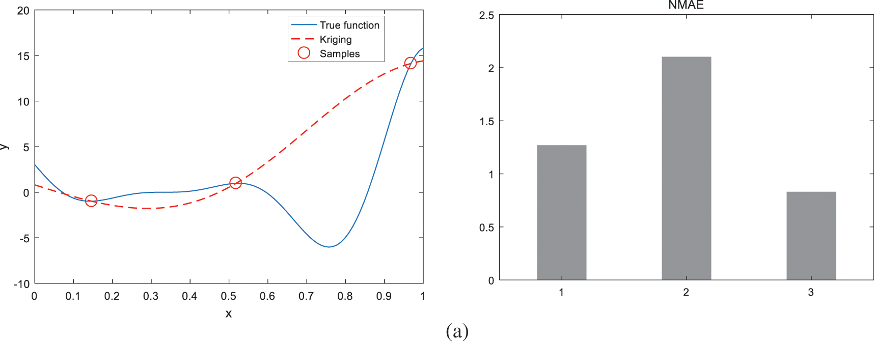
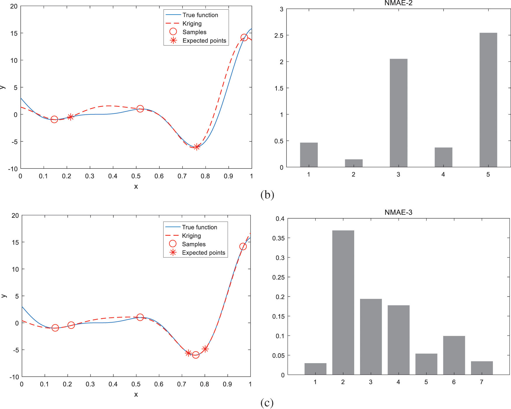
Figure 2: 2 Iterations process. (a) Initial sample distribution and initial model construction, (b) First iteration, (c) Second iteration
Taking the two-dimensional function Branin as an example to explain the construction of the fitting model and iterative optimization in the remodeling domain. The mathematical expression and the corresponding graph of Branin function are shown in Eq. (8) and Fig. 3, respectively.
Figure 3: Branin function
Fig. 4 shows the four iterations of the function. The figure includes the sample update of each iteration, the NMAE values of all sample points and the constructed Kriging model of the function.
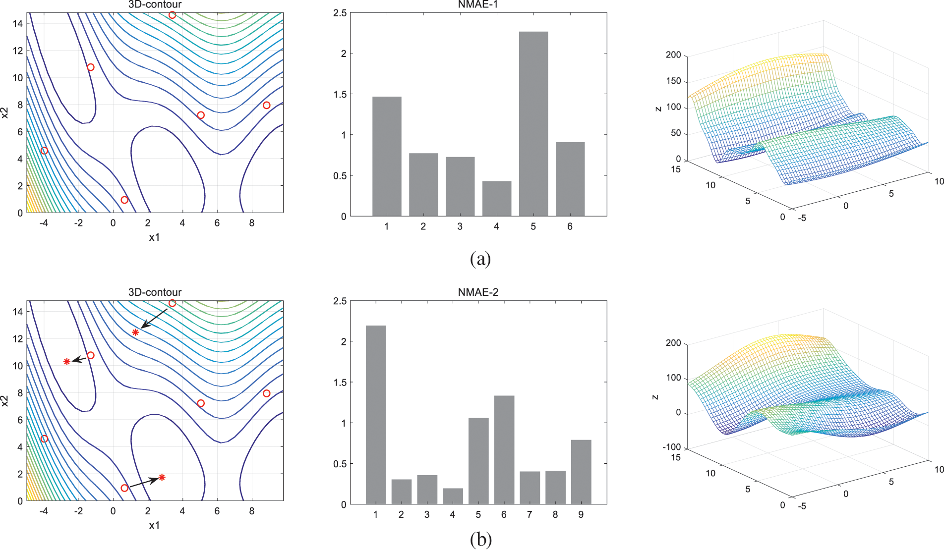
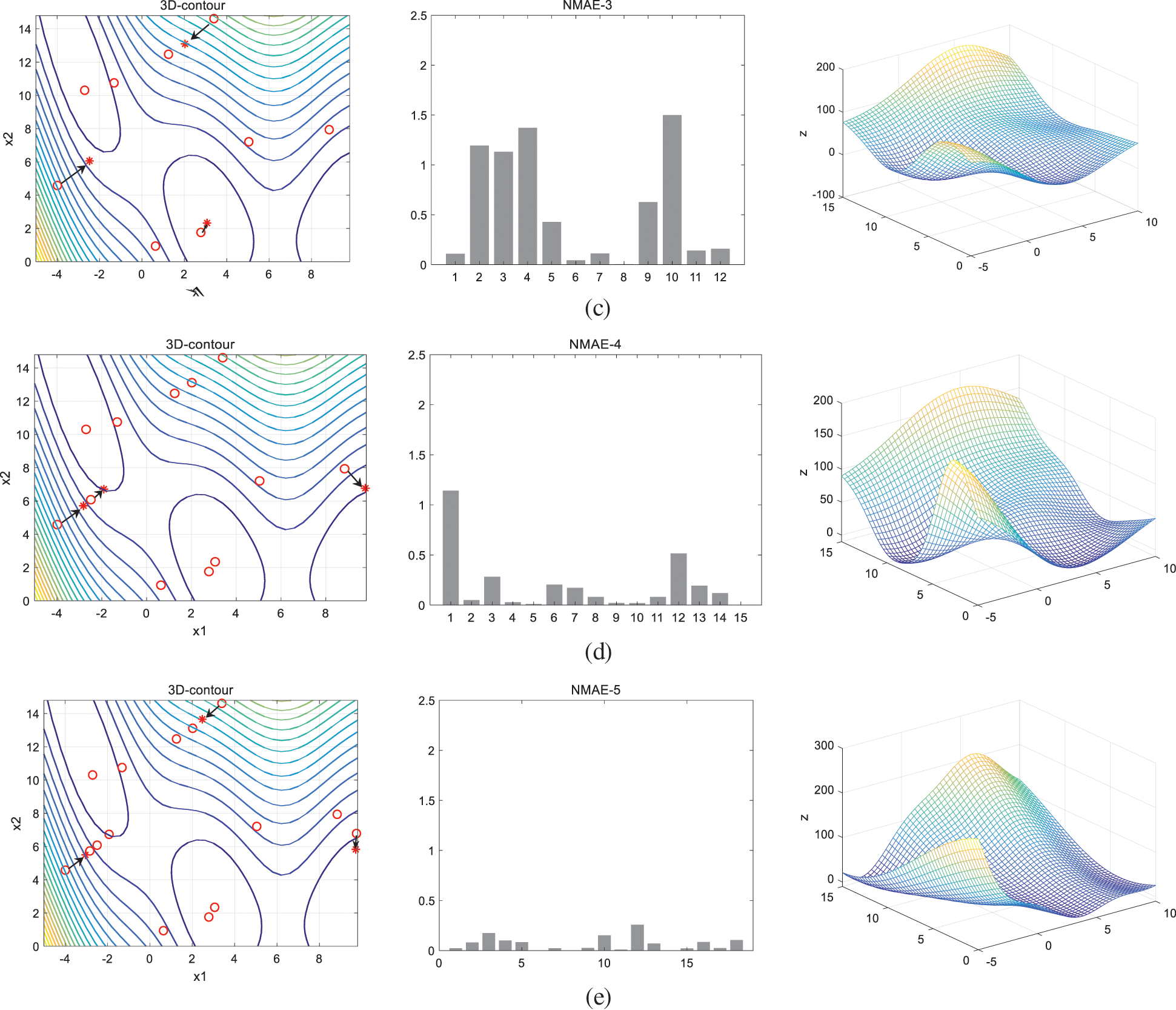
Figure 4: 4 Iterations process. (a) Initial sample distribution and initial model construction, (b) First iteration, (c) Second iteration, (d) Third iteration, (e) Fourth iteration
As shown in Fig. 4a, the function initially selects 6 sample points to construct the surrogate model. The maximum NMAE value of the initial sample is 2.25, the expected number of points generated in each iteration is m = 3, and the expected points are represented by asterisks in the Fig. 4. After four iterations, the total sample size is 18 and the maximum NMAE value is reduced to less than 0.3. The remodeling domain threshold of the first iteration is r = \{2.1419, 2.1419\}, and the remodeling domain threshold of the fourth iteration is r = \{0.9375, 0.9375\}. It can be seen from the Fig. 4 that in the first iteration, there are two reshaped points searched for local extreme values, and the third reshaped point searched for places with dense contour lines. The search direction is the fastest direction perpendicular to the contour lines. This search method meets the original idea of the EGO-LR algorithm, which is to balance local and global search, and also conforms to the point finding characteristics of the EI criterion. The Branin function is relatively simple, so in the second iteration, only one point is searched for local extremum, and the other two points tend to search for areas with high uncertainty in their respective reconstruction domain. In the third and fourth iterations, the maximum NMAE value of sample points is very small, and the algorithm focuses on searching the areas with low fitting accuracy. After the last iteration, the R2 of the surrogate model has reached 0.95, and the fitting model is also close to the real model. Fig. 5 shows the Branin function model initially constructed and the Kriging fitting model for the last iteration.
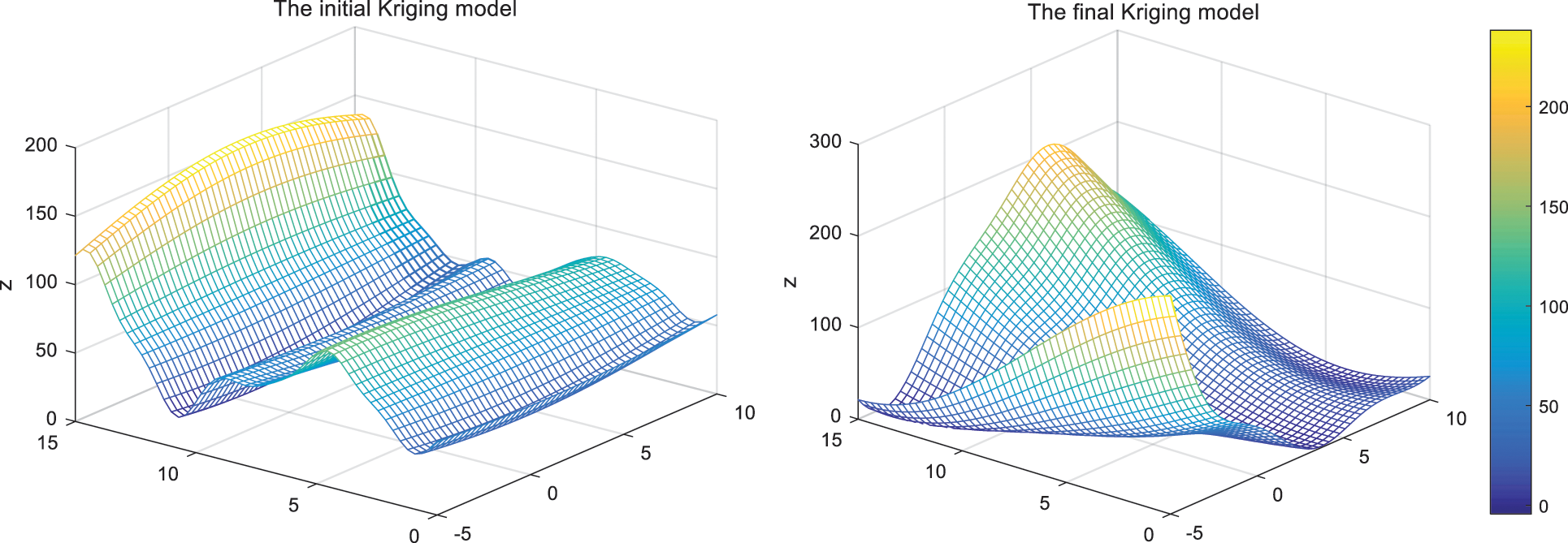
Figure 5: The initial Kriging model and the final Kriging model
2.2 Optimization Comparison between EGO-LR and EGO- PEI Algorithms
The EGO-LR algorithm searches the global optimal value through parallel optimization and generates multiple expectation points in one iteration to reshape the model to ensure the accuracy of optimization. In reference [6], the EGO-PEI algorithm is proposed, which identifies update points by maximizing the PEI function, and selects multiple expected points in each iteration cycle. In this paper, the EGO-LR algorithm is compared with the EGO-PEI algorithm by using 16 benchmark functions from one dimension to eight dimensions under the condition that the same expected points are generated in each iteration. The specific information of the functions is shown in Appendix A. The initial sample points of the same function are the same, and the expected points of each iteration are m = 2, 3, 4, 5. The total number of samples after reaching the convergence condition is shown in Table 1.
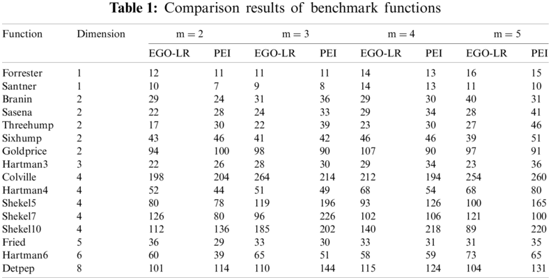
It can be seen from the table that the two algorithms have their own advantages and disadvantages in different functions. For two one-dimensional functions, the EGO-PEI algorithm performs better, and the sample points used are less than the EGO-LR algorithm. Among the 5 two-dimensional functions, four of them are optimized by the EGO-LR algorithm that can converge to the optimal value faster. The function Goldprice is complicated, and the performance of the two algorithms is different due to different iterative expected points. Colville, Shekel5, Shekel7, and Shekel10 are complicated functions with high nonlinearity, large variable space and multiple local extrema. The algorithm needs multiple iterations to obtain enough sample points to obtain the global optimal value. When each iteration generates different number of expected update points to optimize Shekel5, Shekel7 and Shekel10, the total number of samples required by the EGO-LR algorithm are less than that of the EGO-PEI algorithm. Fig. 6 shows the iterative convergence curves of the two algorithms with updating 2, 3, 4 or 5 expected points for some four-dimensional functions each time. The EGO-LR algorithm can quickly jump out of the time-consuming local search and efficiently optimize the global. The EGO-LR algorithm is still applicable to six and eight-dimensional functions. The sample size required in eight-dimensional function Detep is less than that of the EGO-PEI algorithm.
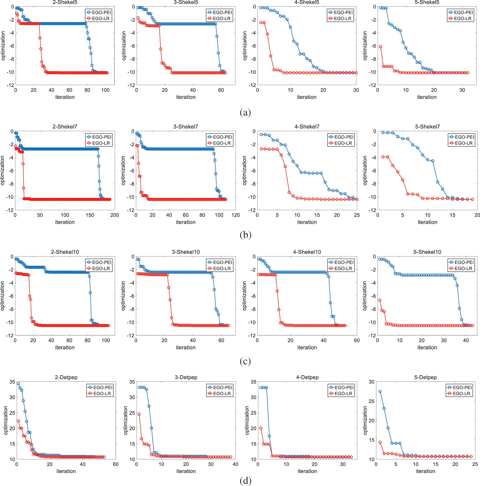
Figure 6: Iterative optimization curve. (a) Shekel5, (b) Shekel7, (c) Shekel10, (d) Detep
The Shekel5, Shekel7 and Shekel10 functions have multiple local optimal values. There are not enough sample points at these local optimal positions which are easy to be mistaken as the expected positions of the next iterative search. It needs to add points many times to jump out of the local optimal positions or always fall into the local domain. The EGO-PEI algorithm performs global optimization from the initial modeling. However, the accuracy of the initial model is very low. When performing multiple optimization operations on these three functions, the EGO-PEI algorithm is easy to fall into a local loop, and very difficult to escape the local search after hundreds of iterations, which means the performance of the EGO-PEI algorithm for complicated functions is unstable. The data of the EGO-PEI algorithm of these three functions in Table 1 and Fig. 6 are selected data that have successfully converged after multiple runs. The EGO-LR algorithm proposed is computationally stable and has little difference in the results of multiple iterations. Although it will fall into the local search of complicated functions, it can quickly jump out of multiple local domains and face the global search. The EGO-LR algorithm not only reduces the time consumption but also can get the accurate optimal value, which is also suitable for high-dimensional functions.
3 Fluid Analysis and Parametric Design of Impeller
Computational Fluid Dynamics (CFD) promotes the experimental research and theoretical analysis of fluid analysis, which is a powerful technology of modern scientific research for simulating and analyzing physical problems such as flow and heat dissipation [24,25]. In this section, the axial-flow impeller and fluid analysis simulation model are established, and the flow characteristics of the outer flow field of the impeller are analyzed by ANSYS CFX. When using the CFD method to simulate actual problems, it is necessary to set the working environment, boundary conditions, and numerical algorithms. These settings will affect the calculation efficiency and accuracy of the model. In the numerical simulation of the model, the SIMPLE algorithm in the finite volume method is used. The core of the algorithm is to modify the pressure field so that the velocity field corresponding to the pressure field meets the solution conditions of the continuous momentum equation.
3.1 Structural Design of Axial Flow Impeller
In engineering practice, according to the different blade outlet installation angles of the impeller, the impeller is divided into three forms: forward inclined type, radial type and backward inclined type [26,27]. In this paper, the backward inclined impeller is used for the structural design and optimization of axial flow impeller that the installation angle of the blade outlet is less than 90 degrees. It has the characteristics of high efficiency, low bearing pressure and high energy conversion rate. The impeller blade adopts arc design, which is conducive to improving blade strength and fluid flow performance. The structure of the impeller is shown in Fig. 7.
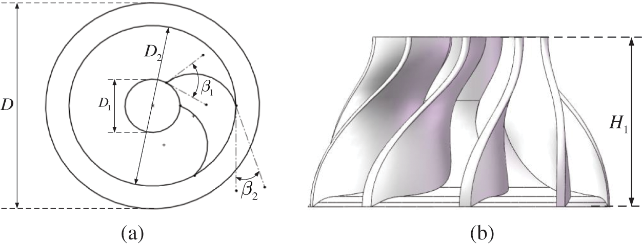
Figure 7: Impeller structure diagram
The function of the impeller is to realize the conversion of energy between fluid kinetic energy and mechanical energy, and improve the speed and flow of fluid. The design of different impeller structural parameters will affect the energy conversion efficiency and the impact force received by the impeller during operation. Ye et al. [28] used the response surface method to optimize the inlet and outlet angle of the impeller blade and improve the efficiency of the pump and impeller. Zhou et al. [29] studied the influence of impeller blade outlet angle on the hydraulic performance of mixed flow pump by a numerical calculation method. According to the literatures on impeller optimization, we consider the main parameters affecting the impeller fluid analysis and carries out the structural design of the impeller. The main structural design parameters of the impeller are shown in Table 2.
Since the main research object of this paper is the performance of impeller blade under the action of flow field and the flow characteristics of flow field, the following text focuses on the design of the relevant parameters of the blade. So the outer flow field diameter, impeller outer diameter and impeller height are set as fixed values to simplify the complexity of blade optimization. The values of parameters are shown in the table.
3.2 Meshing and Model Preprocessing
Before the fluid analysis of the impeller, it is necessary to import the model into ANSYS CFX, and set the boundary conditions and calculation domain of the calculation model. The calculation model and flow field inlet and outlet information are shown in Fig. 8a, the calculation grid division is shown in Fig. 8b, and the boundary condition information is shown in Fig. 8c.
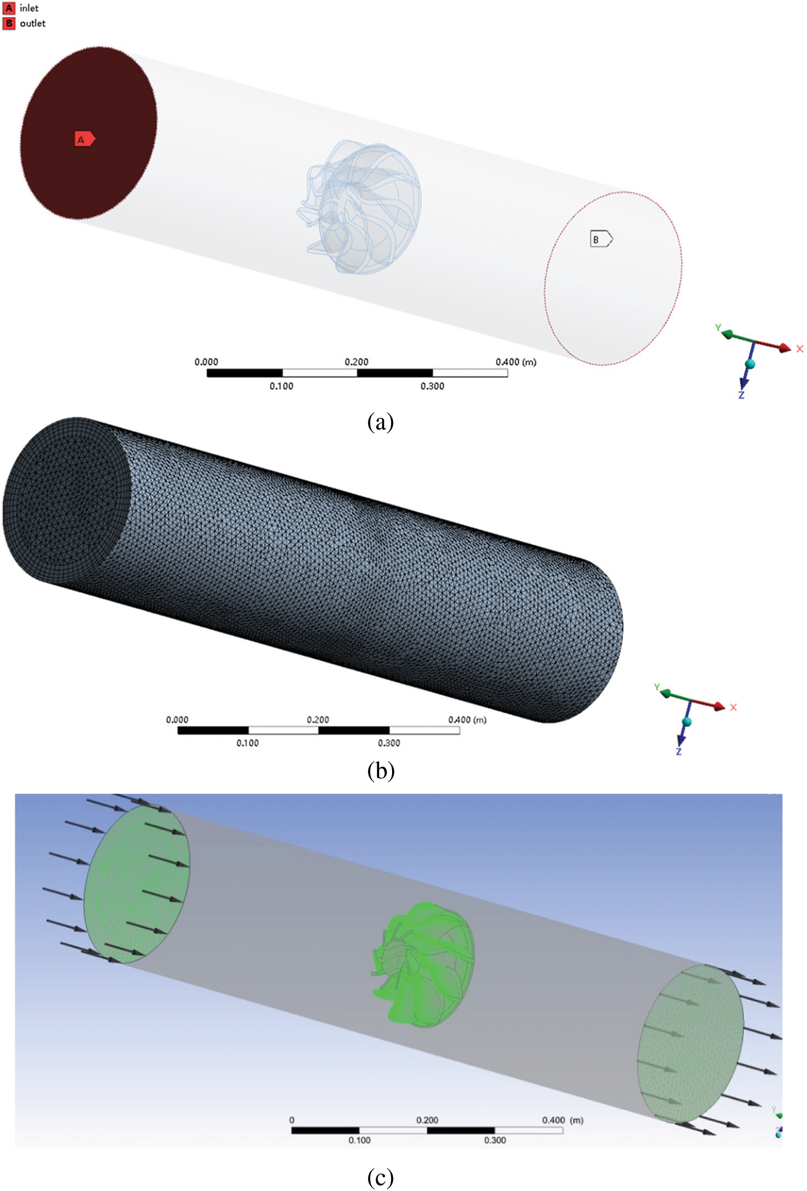
Figure 8: The preprocessing of computational model and computational domain. (a) Geometry configuration, (b) Computational mesh, (c) Boundary settings
In the model processing, the computational domain of unidirectional flow is generated by the way of wall rotation, and the inlet and outlet of fluid are named. Then, the fluid computational domain and impeller model are meshed. Considering the global mesh size, the element quality of mesh is used as the standard to judge whether the meshing is reasonable. The element quality of mesh is expressed as the ratio between the volume and side length of a given cell, and its value is between 0 and 1. 0 is the worst and 1 is the best. In this paper, the average value of the element quality of mesh is more than 0.83, which has far exceeded the reference value of 0.7, so the grid division meets the requirements of fluid analysis. In addition, the number of nodes is 763,539 and the number of elements is 4,002,598. In the pretreatment, the standard k-w turbulence model [30] is used to analyze the external flow field of axial flow impeller. The k-w turbulence model is better for the near wall region and wake region, and the k-w model is considered for the viscous fluid. The working medium is clean water at room temperature. The fluid viscosity is 1. The flow state type is steady-state. The boundary condition of fluid channel inlet is velocity inlet. The flow velocity is v = 5 m/s. The inlet flow rate is Q = 199.835 kg/s, and the outlet boundary is set to standard atmospheric pressure. The wall conditions of the blade and hub of the impeller are designed as rotating wall.
4 Hydrodynamic Analysis and Optimization of Impeller
In the analysis of the external flow field of the impeller, the CFD numerical simulation needs to strictly follow the basic equations of fluid dynamics, deduce the fixed value of the solution parameters related to the impeller, and then conduct fluid analysis and select the optimal value. The numerical simulation method is rigorous, but the simulation results may not be the ideal optimal value, and the mathematical calculation is difficult and takes a lot of time. The introduction of surrogate model optimization theory can reduce the simulations of impeller and fluid dynamics and obtain the ideal optimal solution by transforming the simulation model into fitting function. Since the proposed EGO-LR method shows good convergence in the above test of the benchmark functions with high dimension and great complexity. The hydrodynamic analysis and optimization of Impeller focuses on solving the problems of the complexity of the model and the unknown parameter correlation that affect the fluid flow characteristics. The engineering example has no clear optimization mathematical expression and the target direction of optimization cannot be determined. The application of the EGO-LR method performs auxiliary optimization on the finite element, which can effectively determine the optimization direction. It can avoid searching in unknown local areas, and has a good performance in global optimization.
4.1 The Effect of Blade Number on Impeller Performance
In the component optimization of axial flow fan and the analysis of internal flow field of centrifugal pump, the number of blades of impeller has a great impact on the performance of efficiency and blade load. For the fluid analysis of axial flow impeller, the appropriate number of blades is conducive to improve the fluid flow performance and promote the conversion between fluid kinetic energy and mechanical energy. Fig. 9a shows the variation of the maximum pressure P on the impeller and the maximum fluid velocity V with the number of blades from 3 to 13, and Fig. 9b shows the flow trace cloud diagram when the number of blades is 12.
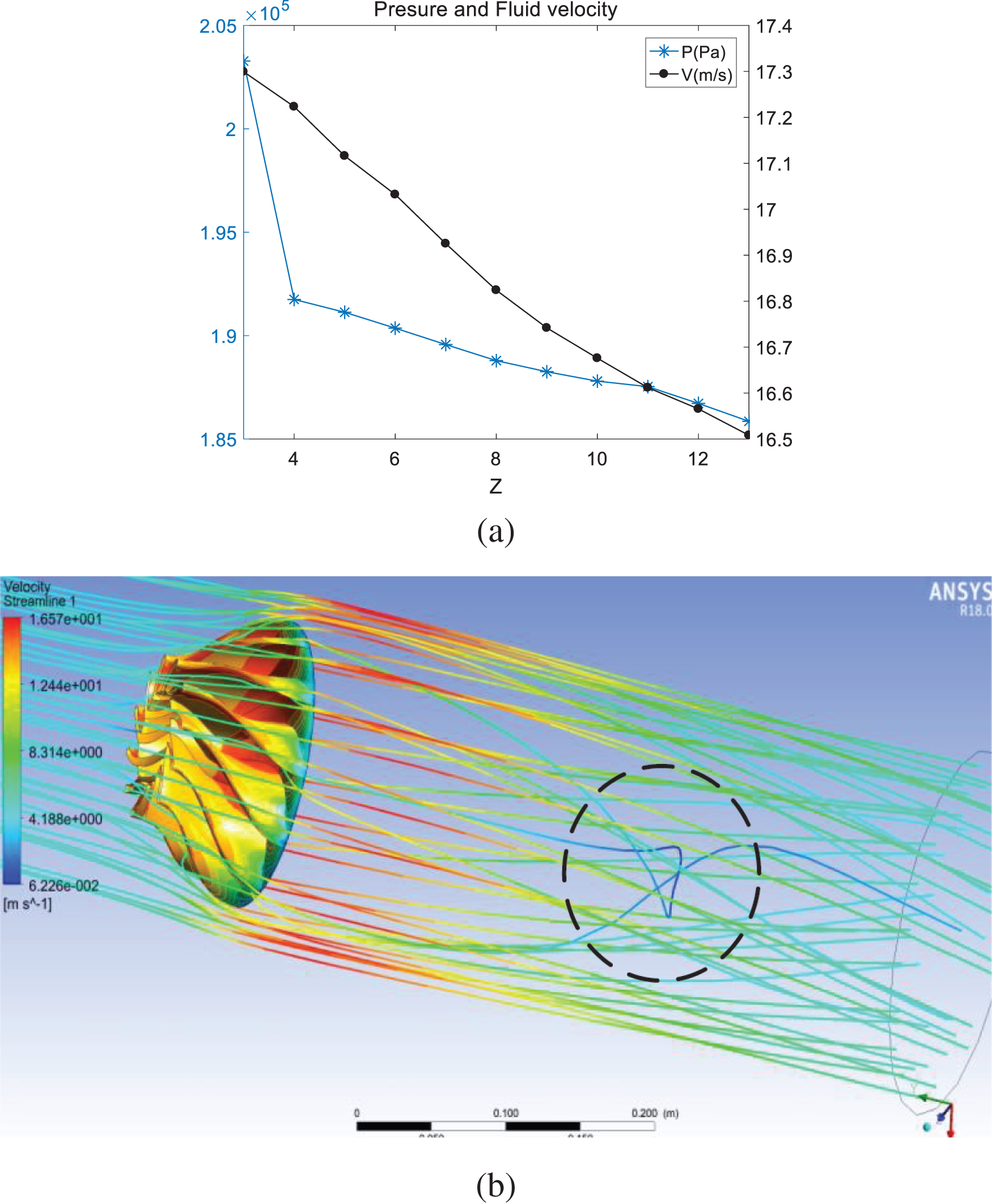
Figure 9: Effect of blade number on impeller flow characteristics
When the steady flow is in contact with the impeller, the angular momentum obtained by the fluid from the impeller depends on the number of times it passes through the impeller. If the number of blades is small, the guiding effect of blades on the fluid is weak, the driving performance of the impeller on fluid is insufficient, and the fluid pressure on a single blade is large. When the number of blades is large, the fluid pressure on a single blade decreases, but the generated fluid hydraulic pressure is insufficient, and the separation and collision times between fluid and blade will increase which results in less energy exchange between blade and fluid. It can be seen from the figure that when the number of blades is 12, there is a large low-speed area near the channel outlet. The minimum flow velocity is 0.0622558 m/s. The exit flow traces are mixed and there is turbulent flow.
4.2 The Optimization Mathematical Model of Impeller
According to the structural analysis of the axial flow impeller, the fluid flow rate is increased to obtain the ideal flow. In order to reduce the fatigue loss of the impeller under long-term working conditions, the original structural parameters of the impeller are optimized by minimizing the maximum pressure (MP) in the impeller structure. Based on the analysis of the influence parameters of the impeller mentioned above, the structural parameter optimization model of axial flow impeller is expressed as follows:
β1, β2, D1 and Z are the main parameters that affect the performance and force distribution of the impeller, respectively.
Based on the analysis of the effect of blade number on impeller performance in the previous section, and considering that the odd and even number of blades will also affect the performance of the impeller [31–33]. The even number of blades will form a symmetrical arrangement, which is not conducive to the balance of the impeller and cause the blade to bear resonance fatigue. To avoid fluid turbulence, improve energy transfer efficiency and minimize the maximum pressure on the blade, the impeller with 9 blades is selected for structural parameter optimization in the following text.
4.3 The Optimization Analysis of Impeller Hydrodynamics Based on the EGO-LR Algorithm
After the number of impeller blades is set, it is necessary to use the EGO-LR algorithm to optimize the blade inlet installation angle, outlet installation angle and inlet diameter. The optimization flow chart is shown in Fig. 10, and the detailed steps are as follows:
(1) Determine the design variables of impeller optimization. Based on the analysis of the influencing parameters of impeller performance, three influencing factors: the installation angle of blade inlet β1, the installation angle of blade outlet β2 and the diameter of blade inlet D1 are determined as design variables.
(2) Random sampling generates initial sample points. The Sobol sequence sampling is used to generate 15 initial sample points and save them to the sample library.
(3) The samples are simulated and analyzed. The 3D software is used for parametric modeling, the model is imported into the hydrodynamic simulation software for simulation analysis to obtain the corresponding response value of the samples.
(4) The Kriging model is constructed and optimized. The Kriging model is constructed by using samples and their response values, and the DE algorithm optimizes the model to obtain the best advantage.
(5) Conduct fluid analysis on the most advantageous parameters through the finite element software to obtain the real maximum pressure value of the impeller, and judge whether the error between the real value and the optimal value of the surrogate model meets the convergence conditions. The convergence conditions are as follows:
where ymin is the best real response value,
(6) If the convergence condition is not met, combined with the surrogate model, the EGO-LR algorithm is used to adaptively add new sample points to the sample library. The three sample points generated in each iteration are added to the sample library and go to Step (3).
(7) Loop simulation and optimization process until the convergence condition is met.
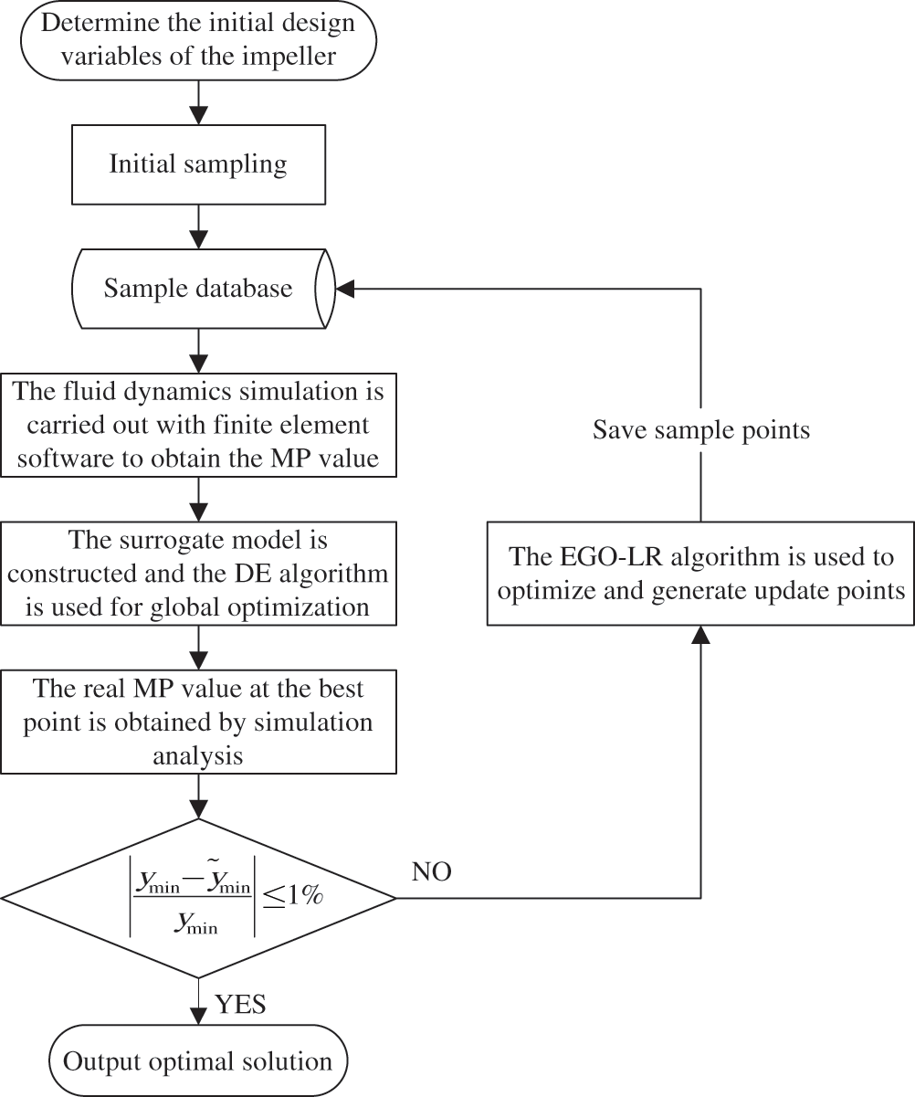
Figure 10: The optimization flow of impeller
Taking the maximum pressure value (MP) carried by the impeller in fluid analysis as the objective function, combined with the EGO-LR algorithm and finite element analysis, the impeller is iteratively optimized to obtain the best structural parameters corresponding to the minimum MP value. The optimization results of each stage before meeting the iterative convergence conditions are shown in Table 4.
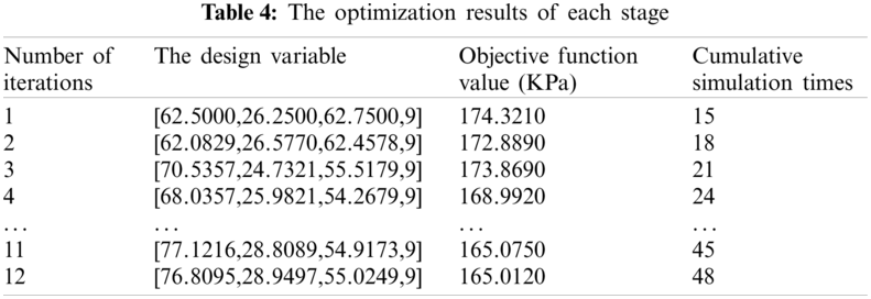
It can be seen from the simulation data in the table that the increasing number of iterations also increases the number of simulations. Since there may be multiple local extremums in the fitting model of the objective function, there is a certain degree of contingency in the optimal objective function value. So the MP value does not necessarily decrease with the increase of iterations. However, the overall change trend of MP value is decline. With the increase of update points, the value of the objective function will tend to be stable, which also reflects the practicability of the black-box optimization problem and the effectiveness of the EGO-LR algorithm. When the optimization is carried out twelve times, a total of 48 simulations are carried out. Fig. 11 shows the plot of residual variance, contour plot of pressure distribution of the impeller and contour plot of the flow trace of the optimal value in the simulation calculation process respectively.
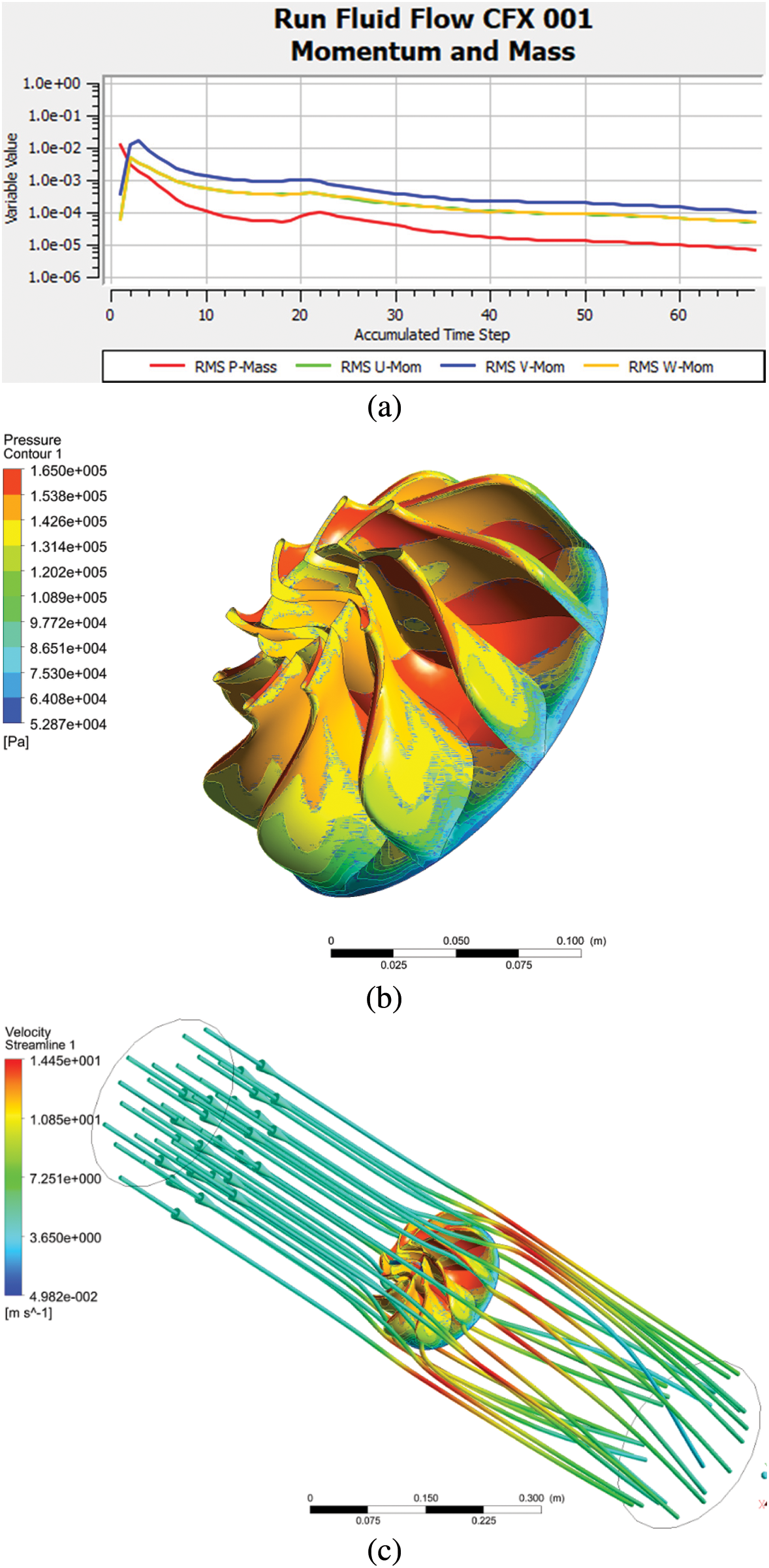
Figure 11: The simulation results. (a) The residual variance curve, (b) Contour plot of pressure distribution of the impeller, (c) Contour plot of the flow trace
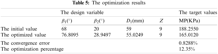
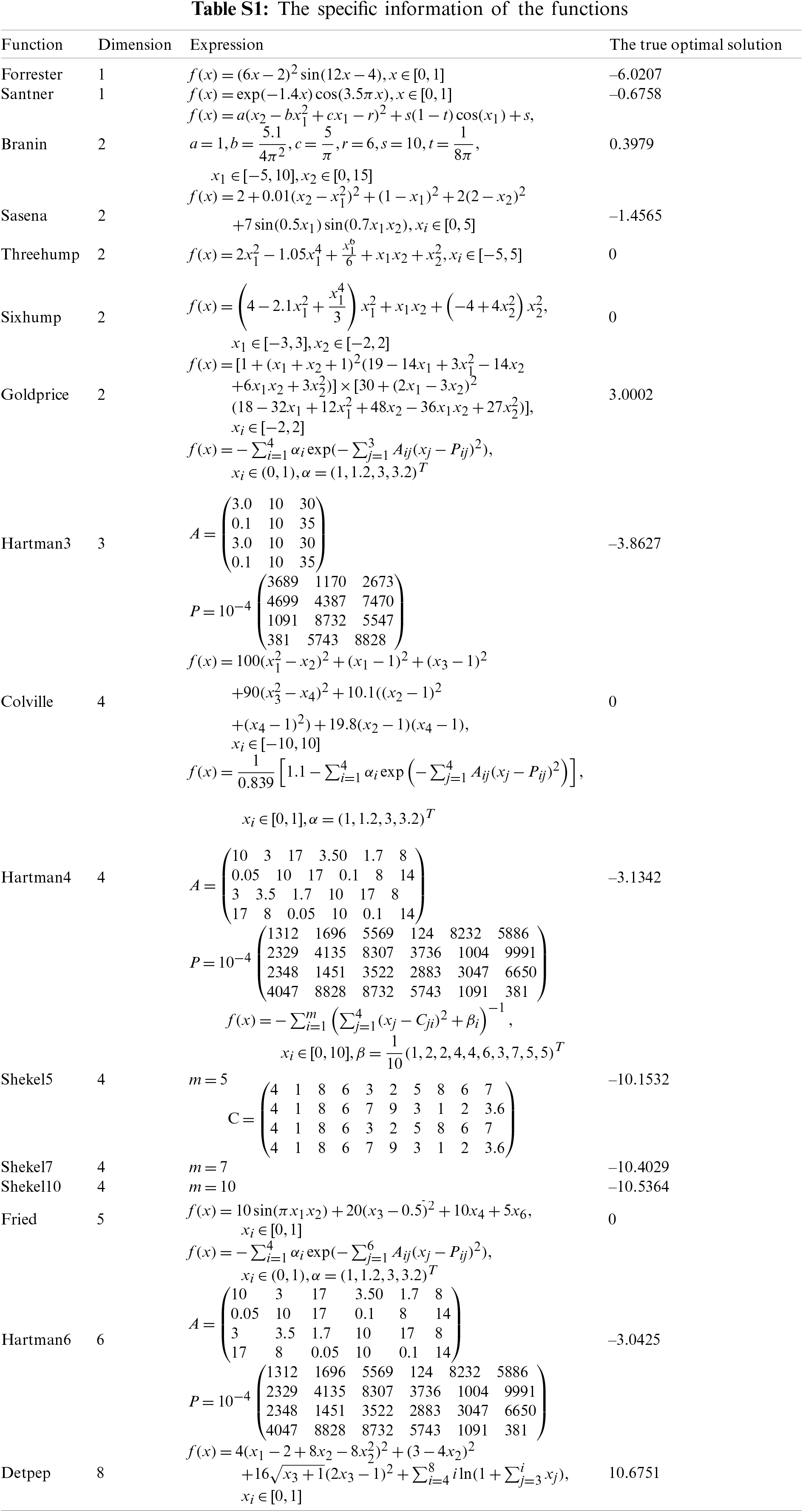
In Fig. 11a, from the analysis of the simulation result graph, the post-processing calculation of the optimal value parameters has good convergence. The convergence residuals are stable below 10-3 and the convergence curve has no oscillation phenomenon. so the calculation results are reliable. The load-bearing pressure distribution of the impeller is shown in Fig. 11b, which different colors represent different pressure values. The dark red color indicates the maximum pressure distribution of the impeller, and the dark blue color indicates the minimum pressure distribution of the impeller. Fig. 11c is the contour plot of the flow trace of the fluid when the impeller is designed with optimal parameters. It can be seen that there is no obvious turbulence phenomenon after the fluid passes through the impeller, and the maximum flow velocity can reach 14.4515 m/s, the initial flow velocity has been greatly improved. The specific information of the initial value before optimization and the optimal value after optimization are shown in Table 5. The MP value in the initial scheme is 188.2550 KPa, and the optimized MP value is 165.0120 KPa. When the convergence conditions are met, the optimized MP value drops by 12.35%, which reduces the load-bearing pressure value of the impeller and ensures that the impeller can run better under load.
Based on the Kriging surrogate model, a new adaptive surrogate model construction method, namely the EGO-LR is proposed. Through the verification and comparison of 16 benchmark functions and the application of optimization design of impeller hydrodynamics, the following conclusions are drawn:
(1) From the view of balancing local and global search, the proposed EGO-LR algorithm efficiently constructs a surrogate model that meets the accuracy requirements and realizes the function of global optimization.
(2) The proposed EGO-LR algorithm can quickly change from local optimization to global optimization when facing the problems of the large range of design variables and multiple local extrema of the objective function. The proposed algorithm starts optimization only when the initial model is successfully constructed and meets a certain accuracy, so that the addition of points and optimization are carried out simultaneously, which improves the optimization efficiency while ensuring accurate requirement.
(3) The proposed method has good performance and practicability in hydrodynamic analysis which reduces the calculation amount and complexity of finite element numerical analysis. The influence of relevant parameters on impeller bearing pressure and impeller performance is analyzed, and the structural parameters of the impeller that meets the boundary conditions in the flow field is optimized. Taking the maximum pressure value as the objective function of the EGO-LR algorithm, the optimal value satisfying the convergence condition is finally obtained through multiple iterations combined with the simulation software.
Funding Statement: This research is supported by the National Natural Science Foundation of China under the Contract No. 51975106.
Conflicts of Interest: The authors declare that they have no conflicts of interest to report regarding the present study.
1. Zhang, W., Gao, Z. H., Zhou, L., Xia, L. (2020). Efficient surrogate-based aerodynamic shape optimization with adaptive design space expansion. Acta Aeronautica et Astronautica Sinica, 41(10), 165–176. DOI 10.7527/S1000-6893.2018.21745. [Google Scholar] [CrossRef]
2. Donald, R. J., Matthias, S., William, J. W. (1998). Efficient global optimization of expensive black-box functions. Journal of Global Optimization, 13(4), 455–492. DOI 10.1023/A:1008306431147. [Google Scholar] [CrossRef]
3. Su, M. M., Zhang, H. Z., Liang, Y. D., He, F. B. (2018). Optimization design of hydraulic valve block pipe structure based on kriging surrogate model. Mechanical Engineer, 10, 22–23+26. [Google Scholar]
4. Zhou, Y. M., Zhang, J. R., Cheng, G. D. (2015). Comparison for two global optimization algorithms based on Kriging surrogate model. Chinese Journal of Computational Mechanics, 32(4), 451–456. DOI 10.7511/jslx201504002. [Google Scholar] [CrossRef]
5. Pramudita, S. P., Koji, S. (2018). On efficient global optimization via universal Kriging surrogate models. Structural and Multidisciplinary Optimization, 57(6), 2377–2397. DOI 10.1007/s00158-017-1867-1. [Google Scholar] [CrossRef]
6. Zhan, D. W., Qian, J. C., Cheng, Y. S. (2017). Pseudo expected improvement criterion for parallel EGO algorithm. Journal of Global Optimization, 68(3), 641–662. DOI 10.1007/s10898-016-0484-7. [Google Scholar] [CrossRef]
7. Jian, X., Luo, Y. J., Gao, Z. H. (2020). A global optimization strategy based on the Kriging surrogate model and parallel computing. Structural and Multidisciplinary Optimization, 62(1), 405–417. DOI 10.1007/s00158-020-02495-6. [Google Scholar] [CrossRef]
8. Ivo, C., Dirk, D., Tom, D. (2014). Fast calculation of multiobjective probability of improvement and expected improvement criteria for Pareto optimization. Journal of Global Optimization, 60(3), 575–594. DOI 10.1007/s10898-013-0118-2. [Google Scholar] [CrossRef]
9. Mohamed, A. B., Nathalie, B., Rommel, G. R., Abdelkader, O., Joseph, M. (2018). Efficient global optimization for high-dimensional constrained problems by using the Kriging models combined with the partial least squares method. Engineering Optimization, 50(12), 2038–2053. DOI 10.1080/0305215X.2017.1419344. [Google Scholar] [CrossRef]
10. Chaudhuri, A., Haftka, R. (2015). Efficient global optimization with adaptive target setting. Aiaa Journal, 52(7), 1573–1578. DOI 10.2514/1.J052930. [Google Scholar] [CrossRef]
11. Zhi, P. P., Xu, Y., Chen, B. Z. (2020). Time-dependent reliability analysis of the motor hanger for EMU based on stochastic process. International Journal of Structural Integrity, 11(3), 453–469. DOI 10.1108/IJSI-07-2019-0075. [Google Scholar] [CrossRef]
12. Li, Y. H., Sheng, Z. Q., Zhi, P. P., Li, D. M. (2021). Multi-objective optimization design of anti-rolling torsion bar based on modified NSGA-III algorithm. International Journal of Structural Integrity, 12(1), 17–30. DOI 10.1108/IJSI-03-2019-0018. [Google Scholar] [CrossRef]
13. Zhu, S. P., Liu, Q., Peng, W. W., Zhang, X. C. (2018). Computational-experimental approaches for fatigue reliability assessment of turbine bladed disks. International Journal of Mechanical Sciences, 142–143(8), 502–517. DOI 10.1016/j.ijmecsci.2018.04.050. [Google Scholar] [CrossRef]
14. Zhi, P. P., Li, Y. H., Chen, B. Z., Li, M., Liu, G. N. (2019). Fuzzy optimization design-based multi-level response surface of bogie frame. International Journal of Structural Integrity, 10(2), 134–148. DOI 10.1108/IJSI-10-2018-0062. [Google Scholar] [CrossRef]
15. Nahal, M., Khelif, R. (2021). A finite element model for estimating time-dependent reliability of a corroded pipeline elbow. International Journal of Structural Integrity, 12(2), 306–321. DOI 10.1108/IJSI-02-2020-0021. [Google Scholar] [CrossRef]
16. Luo, C. Q., Keshtegar, B., Zhu, S. P., Taylan, O., Niu, X. P. (2022). Hybrid enhanced Monte Carlo simulation coupled with advanced machine learning approach for accurate and efficient structural reliability analysis. Computer Methods in Applied Mechanics and Engineering, 388(11), 114218. DOI 10.1016/j.cma.2021.114218. [Google Scholar] [CrossRef]
17. Yi, Z. L., Hou, L., Zhang, Q., Wang, Y. S., You, Y. X. (2019). Geometry optimization of air-assisted swirl nozzle based on surrogate models and computational fluid dynamics. Atomization and Sprays, 29(7), 605–628. DOI 10.1615/AtomizSpr.2019030959. [Google Scholar] [CrossRef]
18. Heo, M. W., Kim, K. Y., Kim, J. H., Choi, Y. S. (2016). High-efficiency design of a mixed-flow pump using a surrogate model. Journal of Mechanical Science and Technology, 30(2), 541–547. DOI 10.1007/s12206-016-0107-8. [Google Scholar] [CrossRef]
19. Lai, X. T., Weng, W. D., Feng, D. J. (2014). Structural optimization of a centrifugal impeller based on a Kriging model. Journal of Shenyang Aerospace University, 31(4), 17–22. DOI 10.3969/j.issn.2095-1248.2014.04.004. [Google Scholar] [CrossRef]
20. Wang, H. P., Jiang, X., Chao, Y., Li, Q., Li, M. Z. et al. (2021). Numerical optimization of horizontal-axis wind turbine blades with surrogate model. Proceedings of the Institution of Mechanical Engineers, Part A: Journal of Power and Energy, 235(5), 1173–1186. DOI 10.1177/0957650920976743. [Google Scholar] [CrossRef]
21. Laurent, G., Lluis, A., Jimenez, R., Elise, A., Fried, H. et al. (2017). Iterative construction of replicated designs based on Sobol’ sequences. Comptes Rendus Mathématique, 355(1), 10–14. DOI 10.1016/j.crma.2016.11.013. [Google Scholar] [CrossRef]
22. Zhang, J., Chowdhury, S., Messac, A. (2012). An adaptive hybrid surrogate model. Structural and Multidisciplinary Optimization, 46(2), 223–238. DOI 10.1007/s00158-012-0764-x. [Google Scholar] [CrossRef]
23. Xu, H. W., Zhang, X., Li, H., Xiang, G. (2021). An ensemble of adaptive surrogate models based on local error expectations. Mathematical Problems in Engineering, 2021, 8857417. [Google Scholar]
24. Li, Y. H., Zhang, C., Yin, H., Cao, Y., Bai, X. N. (2021). Modification optimization-based fatigue life analysis and improvement of EMU gear. International Journal of Structural Integrity, 12(5), 760–772. DOI 10.1108/IJSI-07-2021-0072. [Google Scholar] [CrossRef]
25. Yang, Y. J., Wang, G. H., Zhong, Q. Y., Zhang, H., He, J. J. et al. (2021). Reliability analysis of gas pipeline with corrosion defect based on finite element method. International Journal of Structural Integrity, 12(6), 854–863. DOI 10.1108/IJSI-11-2020-0112. [Google Scholar] [CrossRef]
26. Ge, X. Y. (2017). Structural analysis and optimization design for impeller of backward centrifugal fan. China: Qingdao University. [Google Scholar]
27. Li, G. Y., Yuan, L. Q., Zhao, Z. M., Wang, S. P. (2014). Optimized design of high-efficiency AC motor external fan by computational fluid dynamic method. Advanced Technology of Electrical Engineering and Energy, 33(11), 24–28. [Google Scholar]
28. Ye, D. X., Lai, X. D., Xu, D. H., Zhang, P. (2020). Design and experimental study on leading and trailing blade angle of mixed-flow impeller. Journal of Engineering for Thermal Energy and Power, 35(4), 107–113+145. DOI 10.16146/j.cnki.rndlgc.2020.04.015. [Google Scholar] [CrossRef]
29. Zhou, F. M., Wang, X. F. (2017). The effects of blade stacking lean angle to 1400 MW canned nuclear coolant pump hydraulic performance. Nuclear Engineering and Design, 325(3), 232–224. DOI 10.1016/j.nucengdes.2017.09.024. [Google Scholar] [CrossRef]
30. Sebit, K., Emre, A., Baris, Y., Kody, S. (2014). Computational studies of horizontal axis wind turbines using advanced turbulence models. Marmara Fen Bilimleri Dergisi, 2, 30–40. DOI 10.7240/MJS.2014266488. [Google Scholar] [CrossRef]
31. Rui, Z. M. (2016). Simulation and optimization of fan and impeller flow field based on CFD analysis. China: Southeast University. [Google Scholar]
32. Zhu, S. P., Liu, Q., Zhou, J., Yu, Z. Y. (2018). Fatigue reliability assessment of turbine discs under multi-source uncertainties. Fatigue & Fracture of Engineering Materials & Structures, 41(6), 1291–1305. DOI 10.1111/ffe.12772. [Google Scholar] [CrossRef]
33. Narayanan, G. (2021). Probabilistic fatigue model for cast alloys of aero engine applications. International Journal of Structural Integrity, 12(3), 454–469. DOI 10.1108/IJSI-05-2020-0048. [Google Scholar] [CrossRef]
 | This work is licensed under a Creative Commons Attribution 4.0 International License, which permits unrestricted use, distribution, and reproduction in any medium, provided the original work is properly cited. |