Computer Modeling in Engineering & Sciences

---

DOI: 10.32604/cmes.2022.021225

REVIEW

Explainable Artificial Intelligence–A New Step towards the Trust in Medical Diagnosis with AI Frameworks: A Review

Nilkanth Mukund Deshpande1,2, Shilpa Gite6,7,*, Biswajeet Pradhan3,4,5 and Mazen Ebraheem Assiri4

1Department of Electronics & Telecommunication, Lavale, Symbiosis Institute of Technology, Symbiosis International (Deemed University), Pune, 412115, India
2Electronics & Telecommunication, Vilad Ghat, Dr. Vithalrao Vikhe Patil College of Engineering, Ahmednagar, Maharashtra, 414111, India
3Centre for Advanced Modelling and Geospatial Information Systems (CAMGIS), School of Civil and Environmental Engineering, Faculty of Engineering & IT, University of Technology Sydney, Sydney, 2007, Australia
4Center of Excellence for Climate Change Research, King Abdulaziz University, Jeddah, 21589, Saudi Arabia
5Earth Observation Centre, Universiti Kebangsaan, Institute of Climate Change, Malaysia, Selangor, 43600, Malaysia
6Department of Computer Science, Lavale, Symbiosis Institute of Technology, Symbiosis International (Deemed University), Pune, 412115, India
7Symbiosis Center for Applied Artificial Intelligence (SCAAI), Lavale, Symbiosis International (Deemed University), Pune, 412115, India
*Corresponding Author: Shilpa Gite. Email: shilpa.gite@sitpune.edu.in
Received: 03 January 2022; Accepted: 12 May 2022

1  Introduction

Explainability plays a very important role in various fields of real-life problems [1]. Various software based systems and frameworks are developed by researchers for the solution of the real-life issues of society [2]. The computer vision and related fields cover a variety of problems, such as social, technical, financial, commercial, medicinal, securities, and any other multidisciplinary issues, if any. In addition to different computer vision techniques, some sophisticated and more efficient ways are investigated by researchers. These include machine learning, artificial intelligence, and deep learning techniques. The best thing with these newly developed AI algorithms, is the improved performance in terms of different measures [3–5].

Out of the different real-life problems, medical diagnosis is the most crucial; as it directly affects the human life [6,7]. Diagnosis of any disease should be perfect for providing the proper treatment guidelines to a patient [8]. There are different ways to diagnose the disorder in the medical field. Diagnosis is made from symptoms of some diseases [9]. But in many cases of infections, the generalized symptoms are similar [10]. Thus, it is the prime requirement to use different diagnostics methodologies for the same. Imaging diagnosis is done with traditional image processing [11–13], computer vision [14–18], and sophisticated AI techniques [19–23]. There is a weird trade-off between explainability and accuracy [24], as shown in Fig. 1.

Figure 1: Trade-off between explainability vs. accuracy [33]

As the accuracy increases, explainability falls down [24]. Earlier developed traditional signal and image processing techniques give unsatisfactory results as compared to the newly developed AI techniques [25,26]. But the tragic part related to these techniques is the lack of explainability [27–30]. It could not explain what happens inside the algorithm. On the contrary, conventional image and signal processing techniques explain the algorithms in a magically perfect way [31], to attract trust in the diagnosis, but to provide lesser accuracies [32].

Therefore, researchers forced themselves to use AI techniques for medical diagnosis and related research [34]. It created the need for explainable frameworks for AI techniques [35], in order to make them trusted and commercially adopted for the diagnosis. This paper explains different frameworks for the explainability of AI, machine learning, and deep learning techniques. Initially, different diagnosis methods are discussed, consisting of symptomatic diagnosis, radiology diagnosis, and blood tests diagnosis. Then, the pros and cons of traditional image processing and newly developed AI techniques are presented. Out of the different frameworks of explainability, some frameworks are discussed, including LIME [36], SHAP [37–39], What-if-too l [40–42], Rolex [43,44], Alex-360 [45,46], and so on. A tabular comparison of different techniques applied for the different diagnosis will also be done. Lastly, conclusion and future guidelines are presented.

1.1 Survey Methodology

Medical diagnosis is a very crucial part as the diagnoses are directly affecting the human health. So, this survey needs the articles in the medical diagnosis field utilizing the explainable frameworks to justify the diagnosis. To employ the trust in the diagnosis decisions in the medical field, explainable natures of AI frameworks are needed. So the survey requires retrieving the articles in the medical diagnosis field with XAI frameworks.

1.    Google scholar, is used for searching the articles with the keywords as XAI, explainable AI, explainability, medical, field.

2.    The searched articles are refined by reading them, and keeping the articles related to medical diagnosis using software methods like machine learning, deep learning, and AI techniques.

3.    The articles with XAI frameworks are also added in the survey.

4.    Some cross-references are also obtained from the finalized articles for review paper.

2  Diagnosis Methods in Medical Field

There are two significant ways to detect diseases includes; radiology-consists of various equipment-based imaging [47], and blood tests [48,49] consist of chemical-based tests, equipment-based tests, and microscopic imaging tests. Fig. 1 shows these tests in detail. Imaging technology in health diagnosis has revolutionized healthcare, allowing for early detection of disorders in medical [50–52], fewer unnecessary, intrusive procedures, and improved patient outcomes.

Diagnostic imaging refers to various procedures for examining the body to get the source of an infection causing the illness or damage and confirm a diagnosis, and any signs of a health problem [53,54]. Specific machines and technologies can be used to make images of the activities and structures inside your body. Depending on the body part being examined and your symptoms, your doctor will choose which medical imaging tests are necessary. It is also used by doctors to determine how well a patient responds to fracture or sickness treatment [55].

Many imaging examinations are simple, painless, and non-invasive [56]. However, some will ask you to sit motionless within the machine for an extended period, which can be painful [57]. Some tests expose you to a small amount of radiation [58]. A small camera will be attached to a thin, long tube that will be inserted into your body for further imaging testing. A “scope” is the name for this gadget. The scope will then be passed via a bodily entrance or passageway to allow them to examine a specific organ, such as heart, lungs or the colon. These procedures may necessitate anesthesia.

Fig. 2 shows different diagnoses methods in medical field.

Figure 2: Different diagnostics in medical field

2.1 Radiology Techniques of Diagnosis

2.1.1 Magnetic Resonance Imaging (MRI) [59]

Magnetic resonance imaging (MRI) is a medical imaging method used in radiology to create images of the body’s anatomy and physiological processes. RI scanners are having four types, namely true open, closed, 3 T, and wide bore type.

True Open type has all sides of the MRI to be open. For people who become claustrophobic in a standard MRI machine, it alleviates a lot of the discomfort [60]. Closed type consists of a closed machine, also known as a classic tube machine, requires you to lie down and enter the photos. 3 T is another type of MRI in which the letter “T” stands for Tesla, a unit of measurement used by technologists to determine the strength of magnetic fields. The 3 T MRI is proven to be modern and inventive amongst available MRIs. It is similar to a standard MRI in that it is a closed system. The 3 T MRI requires a reduced amount of time to complete and produces detailed, high-resolution images, allows the radiologist to assess whether there is any serious medical problem [61]. Wide Bore scanner, often known as an “open MRI,” looks similar to a closed MRI but has a larger opening [62].

2.1.2 Magnetic Resonance Angiography (MRA) [63]

This test that produces highly detailed body’s blood arteries images. MRA scans are a type of magnetic resonance imaging (MRI). The MRA uses energy pulses of radio waves and a magnetic field to deliver information that other techniques such as CT, X-ray, and ultrasound are not always able to provide. MRA tests are commonly used to obtain the quality of blood flow and walls of blood vessel in the legs, neck, brain, and kidneys. MRAs are also used by doctors for examination of calcium, aneurysms, and blood clots in the arteries. They may ask for a contrast dye in some cases to boost the definition of the scan images of the blood vessels of patients.

2.1.3 CT Scan [64]

A CT scan is also known as a “cat scan” by doctors. It has a series of X-ray scans or photographs collected from different perspectives. The images of blood arteries and soft tissues inside the body are then created using computer software. CT scans can be used to assess the different organs such as brain, spine, neck, abdomen, and chest. Both hard and soft tissues can be examined by this technique. CT scans provide doctors with images that allow them to make swift medical judgments if necessary. CT scans are routinely performed in both imaging facilities and hospitals due to their high quality. They assist doctors in detecting injury and disorders. Previously, these injuries could be examined through surgeries or autopsy. These techniques are non-invasive and safe, even though they employ low quantities of radiation.

2.1.4 Ultrasound Imaging [65]

Ultrasound imaging, often known as “sonography,” is a safe technique of imaging that produces the bodies inside images. It uses high-frequency waves rather than radiation. Therefore, it proves to be a pregnancy-safe operation. The shape and movement of inner organs, as well as blood flow through channels, are depicted in real-time ultrasound images. In this technique, a transducer—a handheld instrument is placed over the skin during an ultrasound. Internally, it’s sometimes used. It sends sound waves through soft tissue and fluids, echoing or bouncing back as they reach denser surfaces, creating images when the object is more viscous, more ultrasound echoes back.

2.1.5 X-Rays [66]

One of the most well-known and commonly used diagnostic imaging procedures is X-rays. Doctors use these X-rays for looking inside the human body. X-ray machines emit a high-energy beam that cannot penetrate dense tissue or bones but can pass through other body parts. This treatment produces an image that your doctor can use to determine whether or not you have a bone injury.

2.1.6 PET Scan [67]

PET scans are used to diagnose cancer, heart disease, and brain diseases in their early stages. A radioactive tracer that can be injected detects sick cells. APET-CT scan combined generates 3D pictures for a more precise diagnosis.

2.1.7 Mammography [68]

Breast mammograms are X-raying images of the breasts. They use a low-dose X-ray to look for diagnosis of early breast cancer. It may include small lumps that those could not be recognizable easily. Mammograms also reveal changes in breast tissue that could indicate breast cancer at early-stage. Digital mammography is utilized for the diagnosis of nodules of cancer that could be missed by previous methods. Mammograms are the most effective approach to detecting early breast cancer since they can detect it up to a year before symptoms appear.

2.1.8 Bone Density Scan [69]

This is an indirect test for diagnosing the osteoporosis. The process is also known as “bone mineral density testing,” It determines how much bone material is present in your bones per square centimeter.

2.1.9 Arthrogram [70]

When your joints are not functioning properly, it limits your capacity to move and creates problems in routine tasks. So, the arthrogram can be used to diagnose joint abnormalities that may not be detected by other types of imaging. Arthrogram, often known as “arthrography,” is a series of images of the joints acquired with other techniques such as CT, X-ray, MRI, or fluoroscopy.

2.1.10 Myelogram [71]

A myelogram is necessary when a clinician demands detailed imaging of the spinal canal, including the spinal tissue, spinal cord, and surrounding nerves. A myelogram is a process in which a technician injects contrast dye into the spinal canal while taking moving X-ray images with fluoroscopy. The doctor will inspect the area for any abnormalities, such as tumors, infection, or inflammation, as the dye passes through the spaces.

2.2 Chemical Blood Tests and Equipment Based Tests

A blood test determines the number of various chemicals in the body by analyzing a blood sample [72]. Electrolytes, including sodium, potassium, and chloride, are the substances to be detected. Other chemical components include fat contents, protein contents, glucose, and different enzymes are also needed to be detected in the blood sample. Blood chemistry tests inform decisions about how well a person’s organs are functioning. These organs may include kidneys, liver, and other organs.

A high chemical level in the blood can indicate sickness or be a side effect of treatment. Before, during, and after therapy, chemical tests of blood are used to diagnose various illnesses. During the pandemic of COVID-19, chemical tests such as RT-PCR, antigen tests achieved popularity. A binomial model is developed for the laboratories in Northern Cyprus to standardize different parameters of the test (SARS-CoV-2 rRT-PCR) [73].

2.3 Microscopic Imaging Tests

In significant diseases, the morphological characteristics of the blood cells are altered. The conditions like blood cancer-leukemia [74], Thalassemia [75] certain bacterial or viral infections require observing blood cells under a microscope. This type of diagnosis is complex, and it required trained and experienced pathologists for the same [76].

In microscopic imaging, first, the blood sample is taken by a lab technician for analysis. After that, blood staining is performed that outputs the blood smear (slide of blood). This slide is then observed under a good quality microscope for morphological diagnosis, if any.

In medical imaging analysis, there is a need to divide the images into different components. A popular example of microscopic imaging for leukemia detection, in which the image is divided into different parts including white blood cells, red blood cells, blast cells, plasma, etc. [77]. There is a need to have a unique categorization approach in the medical image diagnosis. It consists of inputting the images for study and analysis. The captured images are then pre-processed to remove the noises, if any, and enhance the image quality. The next stage is the segmentation, which outputs the region of interest used for diagnosis purposes. This approach categorizes the input images, and accordingly, the further classification and diagnosis are done. Commonly used features are categorized as intensity-based features, statistical features such as entropy, gray-level co-occurrence matrix (GLCM), local binary pattern, histogram, auto-correlation, transform features such as Gabor features, wavelet features and so on [78].

2.4 Requirement of Software-Based Techniques for Diagnosis

The diagnosis explained in the previous section requires a trained radiologist or a much-trained pathologist for making the diagnosis decisions. The trusted and safest way to perform the diagnosis is the manual intervention of trained technicians in medical imaging. Due to manual diagnosis, it is generally time-consuming and may vary according to the technical experience of the person giving the diagnosis decisions.

To speed up the decision capability and make it independent of the experience or technical superiority of the person, researchers are motivated to develop automated and software-based frameworks for the same [79].

These techniques involve traditional image processing, computer vision methods. With the technological developments in computer vision, a new era of artificial intelligence, machine learning, and deep understanding is started, and researchers started utilizing these frameworks for medical imaging diagnosis [80].

2.5 Traditional Image Processing

Researchers utilize different traditional image processing techniques for medical imaging detection and disease diagnosis. These techniques include different pre-processing techniques such as pre-filtering and noise removal [81], gray scaling [82], and initial image enhancement by edge detections [83], morphological operations [84], etc. In addition to these techniques, some researchers propose segmentation techniques in a broader spectrum are thresholding [85], clustering [86], etc. For the classification of different images for detecting infections and abnormalities, different classification algorithms are employed by researchers, such as decision tree [87], random forest [88], support vector machine [89], and so on.

The main advantage of these systems is their fully explainable nature in diagnostic decisions. Also, these are simple to understand and implement. There is no additional requirement for any GPU-like equipment. Also, the measuring parameters utilizing these systems still need a word of improvement. Therefore, researches are motivated towards the advanced AI techniques, those will prove more efficient in terms of performance.

2.6 Advanced AI and Machine Learning

There are different machine learning, deep learning and AI approaches for medical diagnoses proposed by researchers. Some techniques such as convolution neural network (CNN) [90], recurrent neural network (RNN) [91], U-nets with its advanced modifications [92], deep learning algorithms such as feed-forward [93], CNN [94], NN [95], auto-encoder [96] are employed by the researchers for medical diagnosis.

Fig. 3 shows a simple architecture of convolutional neural network. It has primarily four layers namely input, convolution, pooling and fully connected layer. Finally, it has an output layer. The basic function of CNN is divided into two stages, feature extraction and classification. Feature extraction has first three layers including input layer, convolution n layer and pooling layer. Classification consists of fully connected layer and output layer. A typical Feedforward network is shown in Fig. 4. It has an input layer, hidden layer and an output layer.

Figure 3: CNN architecture [97]

Figure 4: Feedforward network [98]

There are some important architectures such as CNN, Alexnet, Resnet for deep learning diagnosis. LeNet-5 is a 7-level convolutional network that is a first in the field. The ability to handle higher resolution images necessitates larger and more convolutional layers, hence, this method is limited by computational resources. Alexnet increases the depth of the layers compared to Letnet-5 [99]. It includes eight levels, each with its own set of parameters that may be learned. The model comprises of five layers, each of which uses Relu activation, with the exception of the output layer, which uses a combination of max pooling and three fully connected layers [99]. The visualisation of intermediate feature layers and the behaviour of the classifier inspired the design of ZFNet [100]. The filter sizes and stride of the convolutions are both lowered when compared to AlexNet [101]. With an increase in accuracy, Deep CNN architectures compromise the computational costs. This is handled by Inception/Googlenet architecture [102]. VGGNet has 16 convolutional layers and a highly homogeneous design, making it quite appealing. Skip connections, or shortcuts, are used by residual neural networks to jump past some layers. The majority of ResNet models use double- or triple-layer skips with nonlinearities (ReLU) and batch normalization in between [103]. These different architectures of are shown in the figures below.

VGG net has typically VGG 11, VGG 16, and VGG19 architecture. A VGG 16 architecture [104] is shown in Fig. 5. It has the first part containing a series of convolutional layers followed by maxpool layer. It has 05 steps of the same. Finally, it has output layers.

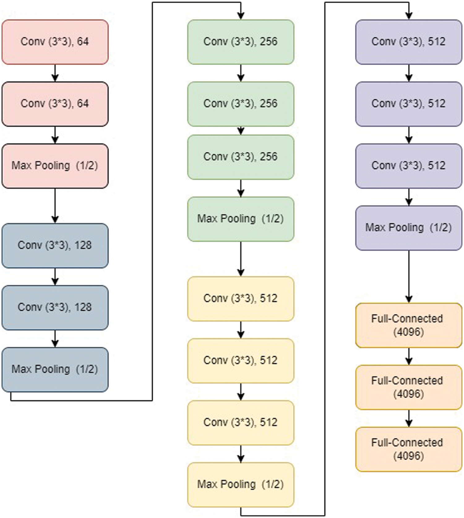
Figure 5: VGG16 architecture [105]

Fig. 6 shows a typical Alexnet architecture. It is shown to have an RGB input image of a particular size. In addition to input layer, it has five convolution layers and some pooling layers as shown in Fig. 6. After the fifth convolution layers, three fully connected layers are present, where the last fully connected layer is the output layer.

Figure 6: Alexnet architecture [106]

As indicated in Fig. 7, Resnet 50 is a variant of a typical Reset model. It has a total of 50 layers. The model has 48 covolutional layers, 01 max pool layer and 01 average pooling layer.

Figure 7: ResNet50 architecture [107]

It has one layer from a convolution with a kernel size of 7 * 7 and 64 distinct kernels, all with a stride of size 2. Following that, we have max pooling with a stride size of 2. There is a 1 * 1, 64 kernel in the next convolution, followed by a 3 * 3, 64 kernel, and finally a 1 * 1, 256 kernel. These three layers are repeated three times in total, giving us nine layers in this phase. Following there is a kernel of 1 * 1, 128, followed by a kernel of 3 * 3, 128, and finally a kernel of 1 * 1, 512. This phase was performed four times, giving us a total of 12 layers. Then there’s a 1 * 1, 256 kernel, followed by 3 * 3, 256 and 1 * 1, 1024 kernels, which are repeated six times for a total of 18 layers. Then a 1 * 1, 512 kernel was added, followed by two more 3 * 3, 512 and 1 * 1, 2048 kernels, for a total of nine layers. After that, we run an average pool and finish with a fully linked layer with 1000 nodes, followed by a softmax function, giving us one layer.

As shown in Fig. 8, the first layer is the input layer, which has a 32 × 32 × 1 feature map. Then there’s the first convolution layer, which has six 5 × 5 filters with a stride of 1. Tanh is the activation function employed at his layer. The final feature map is 28 × 28 × 6 in size. The average pooling layer follows, with a filter size of 2 × 2 and a stride of 1. The feature map that results is 14 × 14 × 6.

Figure 8: LetNet 5 architecture [108]

The number of channels is unaffected by the pooling layer. The second convolution layer follows, with 16 number of 5 × 5 filters and stride 1. Tanh is also the activation function. The output size has been changed to 10 × 10 × 16. The other average pooling layer of 2 × 2 with stride 2 appears once more. As a result, the feature map’s size was reduced to 5 × 5 × 16. The final pooling layer comprises 120 number of 5 × 5 filters with stride 1 and tanh as the activation function. The output size has now increased to 120. The following layer is a completely linked layer with 84 neurons that outputs 84 values, and the activation function is tanh once more. The output layer, which has 10 neurons and uses the Softmax function, is the final layer. The Softmax determines the likelihood that a data point belongs to a specific class. After then, the maximum value is anticipated.

RNN is the recurrent neural network specially designed to deal with the sequential data. It also follows a typical architecture consisting an input layer, hidden layer, and the output layer as indicated in Fig. 9. It takes a word ‘I’ and combines it with ‘i–1’. The same is followed for the word ‘i + 1’. Hence it is called as the recurrent network.

Figure 9: RNN architecture [109]

The convolutional neural network ZFNet is a classic convolutional neural network as shown in Fig. 10. Visualizing intermediate feature layers and the classifier’s operation inspired the design. The filter widths and stride of the convolutions are both lowered when compared to AlexNet. ZF Net utilized 7 × 7 filters, whereas AlexNet used 11 × 11 filters. The idea is that by employing larger filters, we lose a lot of pixel information, which we can keep by utilizing smaller filter sizes in the early convolutional layers. As we go deeper, the number of filters increases. The activation of this network was also done with ReLUs, and it was trained using batch stochastic gradient descent.

Figure 10: ZFnet [110]

In medical diagnosis, more effective deep learning networks, such as Transfer Learning (TL), Ensemble Learning (EL), Convolutional Neural Networks (CNNs), Graph Neural Networks (GNNS), and Explainable Deep Learning Neural Network (xDNNs), perform better. Transfer learning is a machine learning technique in which a model created for one job is utilized as the basis for a model on a different task [111]. Graph Neural Networks (GNNs) are a type of deep learning algorithm that is used to infer data from graphs. GNNs are neural networks that can be applied directly to graphs, making node-level, edge-level, and graph-level prediction jobs simple [112]. Ensembling learning could also prove to be efficient in deep learning applications. The technique of joining multiple learning algorithms to acquire their combined performance is known as ensembling. Individual deep learning models demonstrated competent in the majority of applications, but there is always the possibility of using a collection of deep learning models to complete the same task as an ensembling technique [113].

During the detection and diagnosis of a certain disease via image processing methods, image capturing plays a vital role. Due to some noises and other infections, images may result in wrong predications. So, there are certain pre-processing methods to be applied after image capturing to enhance the sample quality. Generally, gray-scaling, pre-filtering, morphological operations, edge detections are used for pre-processing of samples to enhance its quality for obtaining correct results of disease predications [114].

In early 2019, spread of COVID-19 increased worldwide. Many countries faced different type’s crisis due to this situation. To estimate the parameters and assess the effect of control efforts, the SEIDR epidemic model is utilized. This analysis shows the severity of disease [115]. Different diagnosis methods are studied and introduced by the researchers such as transfer learning, ensemble learning, unsupervised learning and semi-supervised learning, convolutional neural networks, graph neural networks, explainable deep neural networks. Different deep learning networks such as CNNs, RNNs, GNNs, and xDNNs could enhance the diagnosis performance and accuracy [116,117]. Moreover, some approaches optimize the performance of deep learning and machine learning models especially in the crucial diagnosis of COVID-19. Extreme Machine Learning (ELM) with Sine-Cosine optimization [118], Biogeography Based Optimization (BBO) [119], Chimp Optimization Algorithm (ChOA) [120] have proven to be fairly optimizing the performance of machine and deep learning models for COVID-19 diagnosis.

A very popular classical term “calibration” is also applied with machine learning. There are differences in the probability distribution predicted and observed during the training process. A model’s calibration is done to minimize these differences and improvement in the performance of machine learning model. Basic methods of calibration are Sigmoid, and isotonic. In addition, calibration is based on different rules [121].

These approaches are proven to offer remarkable improvements in accuracies and other measuring parameters, as compared to traditional image processing techniques. In spite of the good accuracies, these techniques are not used commercially for different diagnosis purposes. The major cause is the un-explainability of these algorithms. It is very hard to get, what happens inside the black- box of these frameworks. Therefore, there is a need to have explainability and interpretability in these algorithms, in order to support the decision of diagnosis. In the medical domain, the know-how of the diagnostic decision is the prime requirement, to provide the trust in the detection of abnormality. An artificial intelligence generalized methodology is presented in the Section 3, with its black-box nature.

3  Artificial Intelligence

A generalized structure of a machine learning model is shown in Fig. 11. Training data is considered to have the “requests” and the “spam requests”. Spamming is to send unsolicited messages to a certain large group of persons through emails. There are many other ways of spamming including instant messaging, news-groups, search engine, blogs and so on. Spam email is becoming a bigger problem every year, accounting for more than 77 percent of all global email traffic [122]. Out of the messages supplied at the input, spams are to be detected. The same is supplied to the AI model, showing it as a black box. The model consists of an input layer, two hidden layer, and an output layer. The Convolutional Neural Network (CNN) performs the classification of the input data after going through the learning stage. The result is the prediction related to the problem. The prediction in this case gives a good accuracy, but at the cost of black box nature of the classifier model. In the cases like medical diagnosis, it is very important to know the basis of diagnosis. The know-how of the model’s working from inside should be clearly understood, in order to have the trust in prediction of diagnosis. Therefore, the black-box-model needs to be explained from inside to explore that, how the decision of diagnosis is made. The explainable models are used in these cases. There is a popular three-stage model for the explainability (XAI) of AI models.

Figure 11: Generalized frameworks of classification with AI model

There are many machine learning approaches in which it is difficult to get interpretability and explainability directly. These approaches should also require some special XAI techniques for their model’s predictability [123].

3.1 Three Stage Framework of XAI [124]

Fig. 12 shows the three stages of XAI framework, with the first stage as explainable building process, the second stage as explainable decisions, and the third stage having an explainable decision process. The stage-wise explanation of the framework is given below.

Figure 12: Three stage framework of explainable artificial intelligence [124]

3.1.1 Stage 1 (Facilitates Acceptance)

The initial stage of explainability assists in forming a multidisciplinary team of specialists in their domains who are familiar with the AI they are developing. Offline explainability techniques are critical for future AI acceptance and provide possibilities to improve the system.

3.1.2 Stage 2 (Fosters Trust with Users and Supervisors)

Trust is considered to be the most crucial in business, day-to-day life and especially in the medicine diagnosis. The autonomous system and a “micro-controlled” system by its users provide the distinction among each other that is considered to be the trust. The more administration a system demands, the more people it necessitates, and thus the lower it is worth.

When a system does not surprise us, trust is developed when it behaves as per mental model of ours. A system whose users are aware of its limitations is likely to be more beneficial than one whose results are judged unreliable. Any model may be built faster with explanations. That is where the ability to explain AI decisions comes into play. This explains the second stage of the XAI model.

3.1.3 Stage 3(Enables Interoperability with Business Logic)

Stages 1 and 2 are intended to assist humans in gaining a mental understanding of how AIs operate. This allows people to consider how AIs work critically and when to believe and accept their outputs, projections, or suggestions. If you want to scale this up, you’ll need to create business logic that will apply the same “reasoning” to a large number of AIs over time. Interoperability between AIs and other software, particularly business logic software, is the focus of Stage 3.

This is especially crucial when business logic must oversee a large number of increasing AI instances. For example, continual certifiability or collaborative automation between machine learning-based AIs and business rules.

4  Different Frameworks of XAI

4.1 LIME Model [125]

Explanations that can be interpreted locally and are model agnostic-LIME is a technology developed by the University of Washington researchers to get good transparency into about the happenings inside the algorithm. Fig. 13 shows the simple model of LIME.

Figure 13: LIME model

As the dimensions are increasing, it is getting difficult to maintain the local authenticity for the models. On the other hand, LIME deals with the far more manageable problem of the discovery of a model replicating the original model in a local manner.

LIME considers interpretability in both the optimization process and the concept of interpretable representation, allowing for the inclusion of domain specific and task-specific criteria of interpretability. LIME is a modular method for accurately and comprehensibly explaining any model’s predictions. The researchers proposed SP-LIME, used for selecting prominent and non-repetitive predictions that give users a model’s global picture. It accepts the test observations from the AI model. It has three steps, including local, model agnostic, and interpretable ways.

4.2 What-If-Tool [126]

The What-If Tool, developed by the TensorFlow team, is an interactive visual interface for visualizing the datasets and understanding the TensorFlow models’ outputs in a better way, for analyzing the models that have been used. The What-If Tool may be used with XGBoost, and Scikit Learn models in addition to TensorFlow models. The performance of a model can be viewed on a dataset via this tool when it has been deployed.

It allows people to study, evaluate, and compare machine learning models, allowing them to comprehend a classification or regression model better. Everyone from a developer to a product manager to a researcher to a student can use it because of its user-friendly interface and lack of need for sophisticated coding.

Additionally, the dataset may be sliced by features and performance compared across several slices, exposing which subsets of data the model performs best or worst on, which is especially useful for ML fairness studies. The tool aims to provide individuals with a simple, perceptive, and influential way to experiment with a trained machine learning model on a set of data using simply a visual interface. Fig. 14 shows the things to be performed by the What-If Tool.

Figure 14: Things could be performed by What-If-Tool (modified after: https://towardsdatascience.com/using-what-if-tool-to-investigate-machine-learning-models-913c7d4118f)

4.3 DeepLIFT [127]

This method assigns contribution scores based on the difference between each neuron’s activity and its “reference activation.” DeepLIFT considers both positive and negative contributions separately, and it can also show dependencies that other methods miss. In a single backward pass, scores can be computed quickly.

DeepLIFT discusses the difference between an output and a “reference” output, in terms of the difference between an input and a “reference” input. The ‘reference’ input is the default or ‘neutral’ input selected based on what is appropriate for the task at hand.

4.4 Skater [128]

It is a single framework that enables Model Interpretation for all types of models to assist in developing interpretable machine learning systems, which are frequently required for applications related to real-world. Skater is a free, Python library which is open-source that deconstructs the learned structures of a model that could be, otherwise considered to be a black box over a global, and a local scale.

4.5 SHAP [129]

The Shapley Value SHAP, also known as Shapley Additive explanations, is the average marginal contribution of a feature value across all probable coalitions. SHAP’s goal is to figure out how much each attribute contributes to the prediction of an instance x in order to explain it. The SHAP explanation technique, which is based on coalitional game theory, is used to calculate Shapley values. A data instance’s feature values serve as coalition members. Shapley values describe how to distribute the “payout” (= forecast) of a fairway across its various features. A player might be an individual or a group of components.

Pixels are grouped into super-pixels, amongst which the predictions are spread for explaining an image. One of SHAP’s contributions is the Shapley value explanation, which is depicted as an additive feature attribution approach, a linear model.

The formula for SHAP is explained in equation

g(z′)=ϕ0+∑j=1Mϕjzj′(1)

where, g is the model of explanation, z′∈{0, 1}M-coalition vector, M-the maximum size of the coalition, and ϕj∈ R is the feature attribution for jth feature, the Shapley values.

Coalitions are simply featured combinations that are employed for the estimation of the Shapley value of a particular feature. This will prove to be a uniform way of explaining the output of any machine learning model.

SHAP combines game theory and local explanations, bringing together multiple earlier methods and proposing the first additive feature attribution approach based on expectations that are both reliable and local accurate.

Shapley values are the only solution that satisfies the properties of Efficiency, Symmetry, Dummy, and Additivity. SHAP identifies three categories of people who are desired:

Local accuracy:

f(x)=g(x′)=ϕ0+∑j=1Mϕjxj′ (2)

If, ϕ0=EX(f^(x)) and set all xj′ to 1, this is the efficiency property of Shapley,

f(x)=ϕ0+∑j=1Mϕjxj′=EX(f⁡(X))+∑j=1Mϕj(3)

Missingness: An attribution of zero is given to the missing feature. In the equation, a value of zero indicates the missing feature. The missingness attribute assigns missing features a Shapley value of 0. For continuous qualities, this is considered to be a significant practice.

xj′=0⇒ϕj=0(4)

Consistency:

Let fx′(z′)= f(hx(z′), zj′ = 0.

For all inputs, lies between 0 and 1;

fx′(z′)−fx′(z∖j′)≥fx(z′)−fx(z∖j′) (5)

ϕj(f′,x)≥ϕj(f,x)(6)

According to the consistency property, Shapley values vary according to the changes in the contribution of a feature value, independently of other features.

4.6 AIX360 [130]

This is an open-source tool for analyzing and explaining datasets and machine learning models that is free to use. The AI Explainability 360 package is a Python package that offers a vast number of algorithms and proxy explainability measures for many parts of explanations. The AIX360 website has a glossary of words used in the taxonomy and a guidance sheet for users who are not professionals in explainable AI. The AIX360 toolkit intends to provide a consistent, flexible, and user-friendly programming interface and accompanying software architecture to meet the wide range of explainability methodologies required by various stakeholders. The idea is to appeal to data scientists and algorithm engineers, who may not be experts in explainability.

4.7 Activation Atlases [131]

Activation Atlases, developed by Google in partnership with OpenAI, was a revolutionary technique for visualizing the interactions amongst the neural networks, and also the way to grow with knowledge and layers depth. This method was created to investigate convolutional vision networks’ inner workings and obtain a human-interpretable outline of concepts contained within the network’s hidden layers. Individual neurons were the focus of early feature visualization research. By gathering and showing hundreds of thousands of examples of neurons interacting, activation atlases advance from observing individual neurons to visualizing the space those neurons collectively represent.

Humans can use activation atlases to find unanticipated problems in neural networks, where the network depends on erroneous correlations to categorize images, or where repeating a feature between two classes’ results in unexpected flaws. Humans can even “attack” the model by manipulating photos to fool it using this knowledge. Activation atlases performed better than expected, indicating that neural network activations may prove significant to humans. Hence, the interpretability in vision models can be achieved in a meaningful way.

4.8 Rulex Explainable AI [132]

Rolex is a firm that provides easy-to-understand and apply first-order conditional logic rules. The Logic Learning Machine (LLM), Rolex’s main machine learning algorithm, works entirely differently from traditional AI. The solution is built to generate conditional logic rules that forecast the best decision option in straightforward language that process specialists can understand right away. Every prediction is self-explanatory, thanks to Rolex rules. Rolex rules, unlike decision trees and other rule-generating algorithms, are stateless and overlapping.

4.9 GradCAM [133,134]

Gradient-weighted Class Activation Mapping (Grad-CAM) produces a coarse localization map highlighting the essential regions in the image for predicting the idea by using the gradients of any target concept flowing into the final convolutional layer [135]. It is a generalization of Class Activation Mapping (CAM), where CAM needs the use of a global average pooling layer on completely CNN models, whereas CAM can be used on CNN models with fully linked layers. Fig. 15 explains the overview of Grad-CAM explainability framework.

Figure 15: Overview of Grad-CAM [136, Re-drawn after in draw.io]

The image is fed into the network with a target class and the activation maps for the layers of interest are obtained. The coarse Grad-CAM saliency map is computed by back-propagating a one-hot signal with the desired class set to 1 to the rectified convolutional feature maps of interest.

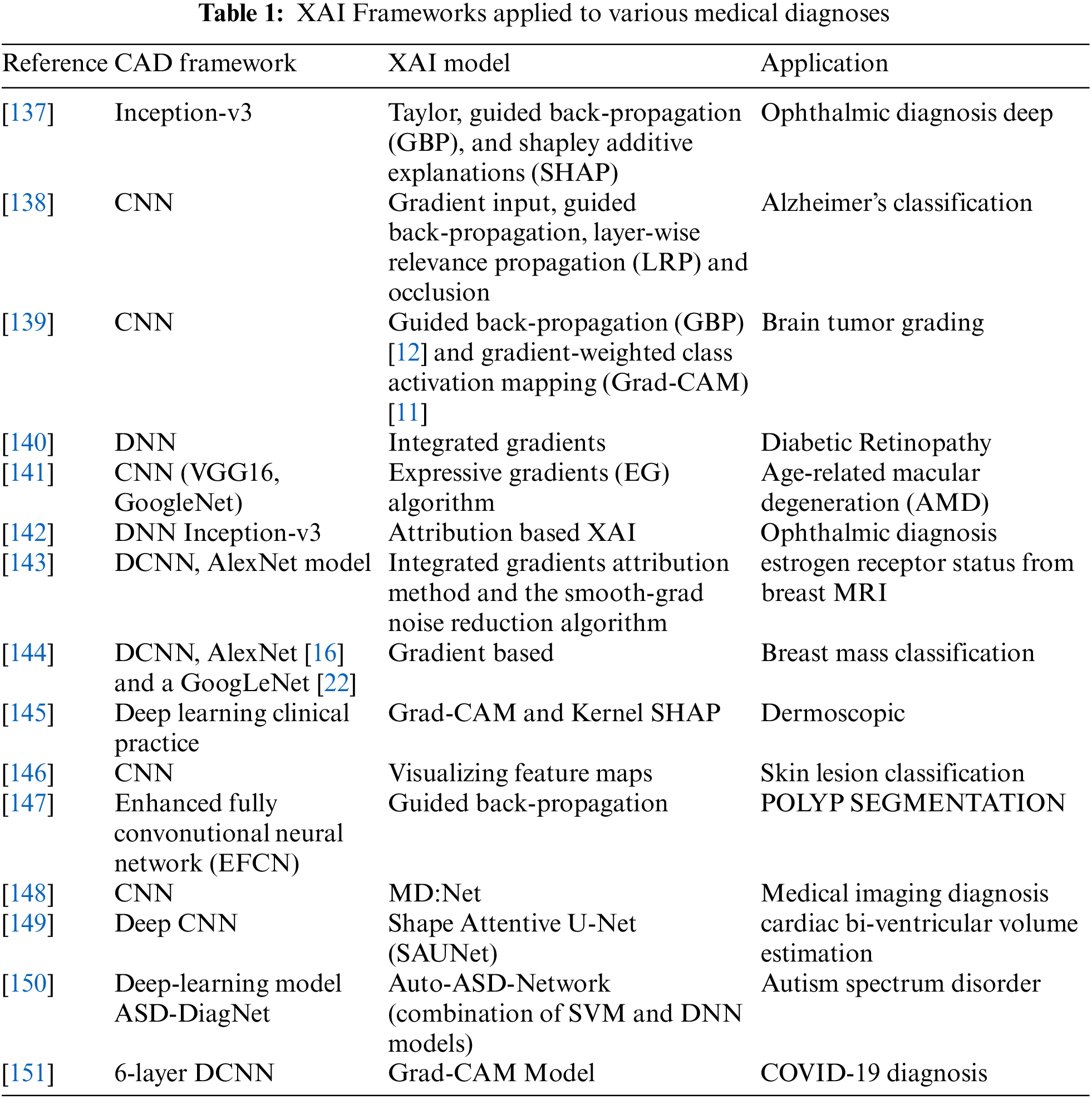
Table 1 shows various frameworks applied by different researchers to different medical diagnoses.

5  Discussion and Future Ahead

It is critical to examine the characteristics of a black-box that can make the wrong judgment for the wrong cause. It is a big problem that might wreak havoc on the system’s performance once it is deployed in the real world. The majority of the methods, particularly the attribution-based ones, are open-source implementations. Explainability, and particularly the attribution methodologies that may be used for a number of business use cases, is gaining commercial interest.

Deep learning models, particularly those employed for medical diagnosis, have made tremendous progress in explaining their decisions. Understanding the aspects that influence a decision can help model designers address reliability challenges, allowing end-users to acquire trust and make better decisions. Almost all of these techniques are aimed at determining local explainability. The majority of deep learning interpretability algorithms use picture classification to generate saliency maps, which highlight the influence of distinct image regions.

The LIME and SHAP methods for visualizing feature interactions and feature importance are by far the most comprehensive and dominant across the literature methods for explaining any black-box model. Grad-CAM, the visual explainability, is getting quite good popularity in terms of explainability and interpretability in recent years.

Apart from the fair explainability of currently developed AI algorithms, certain important aspects are to be considered for the improvement in the trust-worthiness of the medical diagnoses. First thing in line with this is the decision time and the clinical expert’s opinion about accuracies in the diagnosis. It needs to be performed to enhance trust in the implementation and diagnosis. Expert opinion is to be considered in the exploration of the explainability frameworks that may justify the need for the modifications and improvements in the XAI algorithm, if any.

Another line of research could be to combine several modalities in the decision-making process, such as medical pictures and patient records, and attribute model decisions to each of them. This can be used to imitate a clinician’s diagnostic procedure, where photographs and physical parameters of a patient are used to make a decision. Though explainable frameworks are spreading the trust in the medical diagnosis, it still requires a significant amount of exploration in order to adopt them commercially.

6  Conclusion

Medical diagnosis is always very crucial, as depending upon accurate diagnosis, the treatment guidelines are given by the doctors. Symptomatic diagnostics are confusing in many ways, as in most maladies, the symptoms are generally similar. Therefore, imaging tests and blood tests prove to be the better options for the correct diagnosis. Imaging tests always require manual predictions in order to ensure the trust. Manual diagnosis depends on the experience and technical knowledge of the radiologists or pathologists. To provide supportive diagnostics related to the medical field, researchers developed some software frameworks. These frameworks employed image processing, computer vision, and AI techniques, which proved to be more accurate but are unexplainable in nature. In continuation with this, researchers proposed some frameworks for explaining the black-box model of artificial intelligence, machine learning, and deep learning algorithms. The most popular frameworks of XAI are described in this survey. These include LIME, SHAP, what-if-tool, AIX360, activation atlases, Rulex XAI, Grad-CAM, etc. These frameworks are proposed and employed by the researchers to explain the black-box nature of AI models. In any case, it could be believed that explainable artificial intelligence still has many untapped potential areas to examine in the next years.

Acknowledgement: Thanks to two anonymous reviewers for their valuable comments on the earlier version which helped us to improve the overall quality of the manuscript.

Funding Statement: The research is funded by the Centre for Advanced Modeling and Geospatial Information Systems (CAMGIS), Faculty of Engineering & IT, University of Technology Sydney.

Conflicts of Interest: The authors declare that they have no conflicts of interest to report regarding the present study.

References

1. Linardatos, P., Papastefanopoulos, V., & Kotsiantis, S. (2021). Explainable AI: A review of machine learning interpretability methods. Entropy, 23(1), 18. [Google Scholar] [CrossRef]
2. Barros, O. H. (2004). Business information system design based on process patterns and frameworks. Industrial Engineering Department. University of Chile, Santiago. DOI 10.1108/14637150710721122. [CrossRef]
3. Weng, S. F., Reps, J., Kai, J., Garibaldi, J. M., & Qureshi, N. (2017). Can machine-learning improve cardiovascular risk prediction using routine clinical data?. PLoS One, 12(4), [Google Scholar] [CrossRef]
4. Kakadiaris, I. A., Vrigkas, M., Yen, A. A., Kuznetsova, T., & Budoff, M. (2018). Machine learning outperforms ACC/AHA CVD risk calculator in MESA. Journal of the American Heart Association, 7(22), e009476. [Google Scholar] [CrossRef]
5. Liu, T., Fan, W., & Wu, C. (2019). A hybrid machine learning approach to cerebral stroke prediction based on imbalanced medical dataset. Artificial Intelligence in Medicine, 101, 101723. [Google Scholar] [CrossRef]
6. Deshpande, N. M., Gite, S., & Aluvalu, R. (2021). A review of microscopic analysis of blood cells for disease detection with AI perspective. PeerJ Computer Science, 7, e460. [Google Scholar] [CrossRef]
7. Deshpande, N. M., Gite, S. S., Aluvalu, R. (2020). A brief bibliometric survey of leukemia detection by machine learning and deep learning approaches. Library Philosophy and Practice (e-Journal), pp. 1–23.
8. Balogh, E. P., Miller, B. T., Ball, J. R. (2015). Improving diagnosis in health care. Washington DC: National Academies Press. DOI 10.17226/21794. [CrossRef]
9. Corner, J., Hopkinson, J., Fitzsimmons, D., Barclay, S., & Muers, M. (2005). Is late diagnosis of lung cancer inevitable? Interview study of patients’ recollections of symptoms before diagnosis. Thorax, 60(4), 314-319. [Google Scholar] [CrossRef]
10. Shiba, T., Watanabe, T., Kachi, H., Koyanagi, T., & Maruyama, N. (2016). Distinct interacting core taxa in co-occurrence networks enable discrimination of polymicrobial oral diseases with similar symptoms. Scientific Reports, 6(1), 1-13. [Google Scholar] [CrossRef]
11. Tucker, C. C., & Chakraborty, S. (1997). Quantitative assessment of lesion characteristics and disease severity using digital image processing. Journal of Phytopathology, 145(7), 273-278. [Google Scholar] [CrossRef]
12. Petrellis, N. (2017). A smart phone image processing application for plant disease diagnosis. 2017 6th International Conference on Modern Circuits and Systems Technologies (MOCAST), pp. 1–4. Thessaloniki, Greece, IEEE. DOI 10.1109/MOCAST.2017.7937683. [CrossRef]
13. Petrellis, N. (2018). A review of image processing techniques common in human and plant disease diagnosis. Symmetry, 10(7), 270. [Google Scholar] [CrossRef]
14. Khan, N. A., Pervaz, H., Latif, A. K., Musharraf, A. (2014). Unsupervised identification of malaria parasites using computer vision. 2014 11th International Joint Conference on Computer Science and Software Engineering (JCSSE), pp. 263–267. Chonburi, Thailand, IEEE. DOI 10.1109/JCSSE.2014.6841878. [CrossRef]
15. Domingues, I., Sampaio, I. L., Duarte, H., Santos, J. A., & Abreu, P. H. (2019). Computer vision in esophageal cancer: A literature review. IEEE Access, 7, 103080-103094. [Google Scholar] [CrossRef]
16. Doan, M., Case, M., Masic, D., Hennig, H., & McQuin, C. (2020). Label-free leukemia monitoring by computer vision. Cytometry Part A, 97(4), 407-414. [Google Scholar] [CrossRef]
17. Kour, N., & Arora, S. (2019). Computer-vision based diagnosis of Parkinson’s disease via gait: A survey. IEEE Access, 7, 156620-156645. [Google Scholar] [CrossRef]
18. Mengistu, A. D., & Alemayehu, D. M. (2015). Computer vision for skin cancer diagnosis and recognition using RBF and SOM. International Journal of Image Processing, 9(6), 311-319. [Google Scholar]
19. Kaur, S., Singla, J., Nkenyereye, L., Jha, S., & Prashar, D. (2020). Medical diagnostic systems using artificial intelligence (AI) algorithms: Principles and perspectives. IEEE Access, 8, 228049-228069. [Google Scholar] [CrossRef]
20. Brasil, S., Pascoal, C., Francisco, R., dos Reis Ferreira, V. A., & Videira, P. (2019). Artificial intelligence (AI) in rare diseases: Is the future brighter?. Genes, 10(12), 978. [Google Scholar] [CrossRef]
21. Zhou, Y., Wang, F., Tang, J., Nussinov, R., & Cheng, F. (2020). Artificial intelligence in COVID-19 drug repurposing. The Lancet Digital Health, 2, 667-676. [Google Scholar] [CrossRef]
22. Chen, H., Zeng, D., Buckeridge, D. L., Izadi, M. I., & Verma, A. (2009). AI for global disease surveillance. IEEE Intelligent Systems, 24(6), 66-82. [Google Scholar] [CrossRef]
23. Maghded, H. S., Ghafoor, K. Z., Sadiq, A. S., Curran, K., Rawat, D. B. et al. (2020). A novel AI-enabled framework to diagnose coronavirus COVID-19 using smartphone embedded sensors: Design study. 2020 IEEE 21st International Conference on Information Reuse and Integration for Data Science (IRI), pp. 180–187. Las Vegas, NV, USA, IEEE.
24. Frost, N., Moshkovitz, M., Rashtchian, C. (2020). ExKMC: Expanding explainable k-means clustering. arXiv preprint arXiv:2006.02399.
25. Robertson, S., Azizpour, H., Smith, K., & Hartman, J. (2018). Digital image analysis in breast pathology—from image processing techniques to artificial intelligence. Translational Research, 194, 19-35. [Google Scholar] [CrossRef]
26. Razzak, M. I., Naz, S., Zaib, A. (2018). eep learning for medical image processing: Overview. Challenges and the Future Classification in Bioapps, 323–350. DOI 10.1007/978-3-319-65981-7_12. [CrossRef]
27. Kuzlu, M., Cali, U., Sharma, V., & Güler, Ö. (2020). Gaining insight into solar photovoltaic power generation forecasting utilizing explainable artificial intelligence tools. IEEE Access, 8, 187814-187823. [Google Scholar] [CrossRef]
28. Amann, J., Blasimme, A., Vayena, E., Frey, D., & Madai, V. I. (2020). Explainability for artificial intelligence in healthcare: A multidisciplinary perspective. BMC Medical Informatics and Decision Making, 20(1), 1-9. [Google Scholar] [CrossRef]
29. Reddy, S., Allan, S., Coghlan, S., & Cooper, P. (2020). A governance model for the application of AI in health care. Journal of the American Medical Informatics Association, 27(3), 491-497. [Google Scholar] [CrossRef]
30. Samek, W., Müller, K. R. (2019). Towards explainable artificial intelligence. In: Explainable AI: Interpreting, explaining and visualizing deep learning, pp. 5–22. Switzerland AG, Springer, Cham. DOI 10.1007/978-3-030-28954-6. [CrossRef]
31. Pintelas, E., Liaskos, M., Livieris, I. E., Kotsiantis, S., & Pintelas, P. (2020). Explainable machine learning framework for image classification problems: Case study on glioma cancer prediction. Journal of Imaging, 6(6), 37. [Google Scholar] [CrossRef]
32. Nagao, S., Tsuji, Y., Sakaguchi, Y., Takahashi, Y., & Minatsuki, C. (2020). Highly accurate artificial intelligence systems to predict the invasion depth of gastric cancer: Efficacy of conventional white-light imaging, non magnifying narrow-band imaging, and indigo-carmine dye contrast imaging. Gastrointestinal Endoscopy, 92(4), 866-873. [Google Scholar] [CrossRef]
33. Manikonda, P., Poon, K. K., Nguyen, C., Wang, M. H. (2020). Explainable machine learning for credit lending. In: Machine learning term project, pp. 1–62. USA, San Jose State University.
34. Filippetti, F., Franceschini, G., Tassoni, C., & Vas, P. (1998). AI techniques in induction machines diagnosis including the speed ripple effect. IEEE Transactions on Industry Applications, 34(1), 98-108. [Google Scholar] [CrossRef]
35. Hiley, L., Preece, A., Hicks, Y. (2019). Explainable deep learning for video recognition tasks: A framework & recommendations. arXiv preprint arXiv:1909.05667.
36. Dieber, J., Kirrane, S. (2020). Why model why? Assessing the strengths and limitations of LIME. arXiv preprint arXiv:2012.00093.
37. Chromik, M. (2020). Reshape: A framework for interactive explanations in xai based on shap. Proceedings of 18th European Conference on Computer-Supported Cooperative Work European Society for Socially Embedded Technologies (EUSSET), Siegen, Germany. DOI 10.18420/ecscw2020_p06. [CrossRef]
38. Chromik, M., Eiband, M., Buchner, F., Krüger, A., Butz, A. (2021). I think I Get your point, AI! The illusion of explanatory depth in explainable AI. 26th International Conference on Intelligent User Interfaces, pp. 307–317, TX, USA. DOI 10.1145/3397481.3450644. [CrossRef]
39. Lombardi, A., Diacono, D., Amoroso, N., Monaco, A., & Tavares, J. M. (2021). Explainable deep learning for personalized age prediction with brain morphology. Frontiers in Neuroscience, 15, 1-17. [Google Scholar] [CrossRef]
40. Shukla, B., Fan, I. S., & Jennions, I. (2020). Opportunities for explainable artificial intelligence in aerospace predictive maintenance. PHM Society European Conference, 5(1), 11-11. [Google Scholar] [CrossRef]
41. Szczepański, M., Choraś, M., Pawlicki, M., Pawlicka, A. (2021). The methods and approaches of explainable artificial intelligence. International Conference on Computational Science, Springer, Cham. DOI 10.1007/978-3-030-77970-2_1. [CrossRef]
42. Ahn, Y., & Lin, Y. R. (2019). Fairsight: Visual analytics for fairness in decision making. IEEE Transactions on Visualization and Computer Graphics, 26(1), 1086-1095. [Google Scholar] [CrossRef]
43. Al Zamıl, M. G. (2014). A framework for ranking and categorizing medical documents. Republic of Moldova, Lap Lambert Academic Publishing.
44. Zamil, M. G., Samarah, S. (2014). The application of semantic-based classification on big data. In: 2014 5th International Conference on Information and Communication Systems (ICICS), pp. 1–5. Irbid, Jordan, IEEE. DOI 10.1109/IACS.2014.6841941. [CrossRef]
45. Chari, S., Seneviratne, O., Gruen, D. M., Foreman, M. A., Das, A. K., McGuinness, D. L. (2020). Explanation ontology: A model of explanations for user-centered AI. International Semantic Web Conference, pp. 228–243. Springer, Cham.
46. Chaput, R., Cordier, A., Mille, A. (2021). Explanation for humans, for machines, for human-machine interactions? AAAI-2021, Explainable Agency in Artificial Intelligence WS. https://hal.archives-ouvertes.fr/hal-03106286.
47. Giger, M. L. (2002). Computer-aided diagnosis in radiology. Academic Radiology, 9(1), 1-3. [Google Scholar] [CrossRef]
48. Ferrara, G., Losi, M., D’Amico, R., Roversi, P., & Piro, R. (2006). Use in routine clinical practice of two commercial blood tests for diagnosis of infection with mycobacterium tuberculosis: A prospective study. The Lancet, 367(9519), 1328-1334. [Google Scholar] [CrossRef]
49. Kok, L., Elias, S. G., Witteman, B. J., Goedhard, J. G., & Muris, J. W. (2012). Diagnostic accuracy of point-of-care fecal calprotectin and immunochemical occult blood tests for diagnosis of organic bowel disease in primary care: The cost-effectiveness of a decision rule for abdominal complaints in primary care (CEDAR) study. Clinical Chemistry, 58, 6989. [Google Scholar] [CrossRef]
50. di Gioia, D., Stieber, P., Schmidt, G. P., Nagel, D., & Heinemann, V. (2015). Early detection of metastatic disease in asymptomatic breast cancer patients with whole-body imaging and defined tumour marker increase. British Journal of Cancer, 112(5), 809-818. [Google Scholar] [CrossRef]
51. Kaufmann, B. A., Carr, C. L., Belcik, J. T., Xie, A., & Yue, Q. (2010). Molecular imaging of the initial inflammatory response in atherosclerosis: Implications for early detection of disease. Arteriosclerosis, Thrombosis, and Vascular Biology, 30(1), 54-59. [Google Scholar] [CrossRef]
52. Teipel, S. J., Grothe, M., Lista, S., Toschi, N., & Garaci, F. G. (2013). Relevance of magnetic resonance imaging for early detection and diagnosis of Alzheimer disease. Medical Clinics, 97(3), 399-424. [Google Scholar] [CrossRef]
53. Armstrong, P., Wastie, M., Rockall, A. G. (2010). Diagnostic imaging. USA: John Wiley & Sons.
54. Angtuaco, E. J., Fassas, A. B., Walker, R., Sethi, R., & Barlogie, B. (2004). Multiple myeloma: Clinical review and diagnostic imaging. Radiology, 231(1), 11-23. [Google Scholar] [CrossRef]
55. de Paulis, F., Cacchio, A., Michelini, O., Damiani, A., & Saggini, R. (1998). Sports injuries in the pelvis and hip: Diagnostic imaging. European Journal of Radiology, 27, S49-S59. [Google Scholar] [CrossRef]
56. Gore, J. C. (2014). Biomedical imaging, woodhead publishing. DOI 10.1016/B978-0-85709-127-7.50015-6. [CrossRef]
57. Neurological diagnostic tests and procedures (2021). https://www.ninds.nih.gov/Disorders/Patient-Caregi-ver-Education/Fact-Sheets/Neurological-Diagnostic-Tests-and-Procedures-.
58. Davies, H. E., Wathen, C. G., & Gleeson, F. V. (2011). The risks of radiation exposure related to diagnostic imaging and how to minimize them. BMJ, 342, d947. [Google Scholar] [CrossRef]
59. Polygerinos, P., Ataollahi, A., Schaeffter, T., Razavi, R., & Seneviratne, L. D. (2011). MRI-compatible intensity-modulated force sensor for cardiac catheterization procedures. IEEE Transactions on Biomedical Engineering, 58(3), 721-726. [Google Scholar] [CrossRef]
60. Schmidt, A., Stockton, D. J., Hunt, M. A., Yung, A., & Masri, B. A. (2020). Reliability of tibiofemoral contact area and centroid location in an upright, open MRI. BMC Musculoskeletal Disorders, 21(1), 1-9. [Google Scholar] [CrossRef]
61. Fischer, G. S., DiMaio, S. P., Iordachita, I. I., Fichtinger, G. (2007). Robotic assistant for transperineal prostate interventions in 3 T closed MRI. International Conference on Medical Image Computing and Computer-Assisted Intervention, pp. 425–433. Springer, Berlin, Heidelberg. DOI 10.1007/978-3-540-75757-3_52. [CrossRef]
62. Liney, G. P., Owen, S. C., Beaumont, A. K., Lazar, V. R., & Manton, D. J. (2013). Commissioning of a new wide-bore MRI scanner for radiotherapy planning of head and neck cancer. The British Journal of Radiology, 86(1027), [Google Scholar] [CrossRef]
63. Hartung, M. P., Grist, T. M., & François, C. J. (2011). Magnetic resonance angiography: Current status and future directions. Journal of Cardiovascular Magnetic Resonance, 13(1), 1-11. [Google Scholar] [CrossRef]
64. Ramakrishnan, S., Nagarkar, K., DeGennaro, M., Srihari, M., Courtney, A. K. et al. (2004). A study of the ct scan area of a healthcare provider. Proceedings of the 2004 Winter Simulation Conference, vol. 2, pp. 2025–2031. IEEE. DOI 10.1109/WSC.2004.1371565. [CrossRef]
65. Genc, A., Ryk, M., Suwała, M., Żurakowska, T., & Kosiak, W. (2016). Ultrasound imaging in the general practitioner’s office–a literature review. Journal of Ultrasonography, 16(64), 78. [Google Scholar] [CrossRef]
66. Hessenbruch, A. (2002). A brief history of x-rays. Endeavour, 26(4), 137-141. [Google Scholar] [CrossRef]
67. Arisawa, H., Sato, T., & Hata, S. (2008). PET-CT imaging and diagnosis system following doctor’s method. HEALTHINF, 1, 258-261. [Google Scholar]
68. Sampat, M. P., Markey, M. K., Bovik, A. C. (2005). Computer-aided detection and diagnosis in mammography. In: Handbook of image and video processing, pp. 1195–1217. DOI 10.1016/B978-012119792-6/50130-3. [CrossRef]
69. Schoenau, E., Saggese, G., Peter, F., Baroncelli, G. I., & Shaw, N. J. (2004). From bone biology to bone analysis. Hormone Research in Paediatrics, 61(6), 257-269. [Google Scholar] [CrossRef]
70. Schmid, M. R., Nötzli, H. P., Zanetti, M., Wyss, T. F., & Hodler, J. (2003). Cartilage lesions in the hip: Diagnostic effectiveness of MR arthrography. Radiology, 226(2), 382-386. [Google Scholar] [CrossRef]
71. Sandow, B. A., & Donnal, J. F. (2005). Myelography complications and current practice patterns. American Journal of Roentgenology, 185(3), 768-771. [Google Scholar] [CrossRef]
72. Deshpande, N. M., Gite, S. S., Aluvalu, R. (2022). Microscopic analysis of blood cells for disease detection: A review. In: Tracking and preventing diseases with artificial intelligence, vol. 206, pp. 125–151. DOI 10.1007/978-3-030-76732-7_6. [CrossRef]
73. Sultanoglu, N., Gokbulut, N., Sanlidag, T., Hincal, E., & Kaymakamzade, B. (2021). A binomial model approach: Comparing the R0 values of SARS-CoV-2 rRT-PCR data from laboratories across northern Cyprus. Computer Modeling in Engineering & Sciences, 128(2), 717-729. [Google Scholar] [CrossRef]
74. Saritha, M., Prakash, B. B., Sukesh, K., Shrinivas, B. (2016). Detection of blood cancer in microscopic images of human blood samples: A review. 2016 International Conference on Electrical, Electronics, and Optimization Techniques (ICEEOT), pp. 596–600. Chennai, India, IEEE. DOI 10.1109/ICEEOT.2016.7754751. [CrossRef]
75. Bhowmick, S., Das, D. K., Maiti, A. K., & Chakraborty, C. (2012). Computer-aided diagnosis of thalassemia using scanning electron microscopic images of peripheral blood: A morphological approach. Journal of Medical Imaging and Health Informatics, 2(3), 215-221. [Google Scholar] [CrossRef]
76. Deshpande, N. M., Gite, S. S. (2021). A brief bibliometric survey of explainable ai in medical field. library philosophy and practice. https://digitalcommons.unl.edu/libphilprac/5310.
77. Deshpande, N. M., Gite, S., Pradhan, B. S., Kotecha, K., & Alamri, A. (2022). Improved otsu and kapur approach for white blood cells segmentation based on LebTLBO optimization for the detection of leukemia[J]. Mathematical Biosciences and Engineering, 19(2), 1970-2001. [Google Scholar] [CrossRef]
78. Vidya, M. S., Shastry, A. H., Mallya, Y. (2020). Automated detection of intracranial hemorrhage in noncontrast head computed tomography. Advances in Computational Techniques for Biomedical Image Analysis, pp. 71–98. Cambridge, Massachusetts: Academic Press.
79. Sutton, R. T., Pincock, D., Baumgart, D. C., Sadowski, D. C., & Fedorak, R. N. (2020). An overview of clinical decision support systems: Benefits, risks, and strategies for success. NPJ Digital Medicine, 3(1), 1-10. [Google Scholar] [CrossRef]
80. Hafiz, A. M., Bhat, G. M. (2020). A survey of deep learning techniques for medical diagnosis. In: Information and communication technology for sustainable development, pp. 161–170. Springer, Singapore. DOI 10.1007/978-981-13-7166-0_16. [CrossRef]
81. Viola, I., Kanitsar, A., Groller, M. E. (2003). Hardware-based nonlinear filtering and segmentation using high-level shading languages, pp. 309–316. Seattle, WA, USA, IEEE. DOI 10.1109/VISUAL.2003.1250387. [CrossRef]
82. Raja, N. S., Fernandes, S. L., Dey, N., Satapathy, S. C., Rajinikanth, V. (2018). Contrast enhanced medical mri evaluation using tallis entropy and region growing segmentation. Journal of Ambient Intelligence and Humanized Computing, 1–12. DOI 10.1007/s12652-018-0854-8. [CrossRef]
83. Piórkowski, A. (2016). A statistical dominance algorithm for edge detection and segmentation of medical images. Conference of Information Technologies in Biomedicine, pp. 3–14. Springer, Cham. DOI 10.1007/978-3-319-39796-2_1. [CrossRef]
84. Chen, C. W., Luo, J., & Parker, K. J. (1998). Image segmentation via adaptive K-mean clustering and knowledge-based morphological operations with biomedical applications. IEEE Transactions on Image Processing, 7(12), 1673-1683. [Google Scholar] [CrossRef]
85. Senthilkumaran, N., & Vaithegi, S. (2016). Image segmentation by using thresholding techniques for medical images. Computer Science & Engineering: An International Journal, 6(1), 1-13. [Google Scholar] [CrossRef]
86. Ng, H. P., Ong, S. H., Foong, K. W., Goh, P. S., Nowinski, W. L. (2006). Medical image segmentation using k-means clustering and improved watershed algorithm. IEEE Southwest Symposium on Image Analysis and Interpretation, pp. 61–65. Denver, Colorado, IEEE. DOI 10.1109/SSIAI.2006.1633722. [CrossRef]
87. Rajendran, P., Madheswaran, M. (2010). Hybrid medical image classification using association rule mining with decision tree algorithm. arXiv preprint arXiv:1001.3503.
88. Désir, C., Bernard, S., Petitjean, C., Heutte, L. (2012). A random forest based approach for one class classification in medical imaging. International Workshop on Machine Learning in Medical Imaging, pp. 250–257. Springer, Berlin, Heidelberg. DOI 10.1007/978-3-642-35428-1_31. [CrossRef]
89. Abdullah, N., Ngah, U. K., Aziz, S. A. (2011). Image classification of brain MRI using support vector machine. IEEE International Conference on Imaging Systems and Techniques, pp. 242–247. Batu Ferringhi, Malaysia, IEEE. DOI 10.1109/IST.2011.5962185. [CrossRef]
90. Arena, P., Basile, A., Bucolo, M., & Fortuna, L. (2003). Image processing for medical diagnosis using CNN. Nuclear Instruments and Methods in Physics Research Section A: Accelerators, Spectrometers, Detectors and Associated Equipment, 497(1), 174-178. [Google Scholar] [CrossRef]
91. Jagannatha, A. N., Yu, H. (2016). Bidirectional RNN for medical event detection in electronic health records. Proceedings of the 2016 Conference of the North American Chapter of the Association for Computational Linguistics: Human Language Technologies, pp. 473–482. San Diego, California. DOI 10.18653/v1/N16-1056. [CrossRef]
92. Du, G., Cao, X., Liang, J., Chen, X., & Zhan, Y. (2020). Medical image segmentation based on u-net: A review. Journal of Imaging Science and Technology, 64(2), [Google Scholar] [CrossRef]
93. Gaonkar, B., Hovda, D., Martin, N., & Macyszyn, L. (2016). Deep learning in the small sample size setting: Cascaded feed forward neural networks for medical image segmentation, in medical imaging: Computer-aided diagnosis. Medical Imaging 2016: Computer-Aided Diagnosis, 9785, 97852I. [Google Scholar] [CrossRef]
94. Bakator, M., & Radosav, D. (2018). Deep learning and medical diagnosis: A review of literature. Multimodal Technologies and Interaction, 2(3), 47. [Google Scholar] [CrossRef]
95. Shen, D., Wu, G., & Suk, H. I. (2017). Deep learning in medical image analysis. Annual Review of Biomedical Engineering, 19, 221-248. [Google Scholar] [CrossRef]
96. Chen, M., Shi, X., Zhang, Y., Wu, D., & Guizani, M. (2017). Deep features learning for medical image analysis with convolutional autoencoder neural network. IEEE Transactions on Big Data, 7(4), 750-758. [Google Scholar] [CrossRef]
97. Ali, L., Alnajjar, F., Jassmi, H. A., Gochoo, M., & Khan, W. (2021). Performance evaluation of deep CNN-based crack detection and localization techniques for concrete structures. Sensors, 21(5), 1688. [Google Scholar] [CrossRef]
98. Hakim, S. J. S., Noorzaei, J., Jaafar, M. S., Jameel, M., & Mohammadhassani, M. (2011). Application of artificial neural networks to predict compressive strength of high strength concrete. International Journal of Physical Sciences, 6(5), 975-981. [Google Scholar]
99. Hao, P., Zhai, J. H., Zhang, S. F. (2017). A simple and effective method for image classification. 2017 International Conference on Machine Learning and Cybernetics (ICMLC), vol. 1, pp. 230–235. Ningbo, China, IEEE.
100. Alom, M. Z., Taha, T. M., Yakopcic, C., Westberg, S., & Sidike, P. (2019). A state-of-the-art survey on deep learning theory and architectures. Electronics, 8(3), 292. [Google Scholar] [CrossRef]
101. Singh, S. P., Wang, L., Gupta, S., Goli, H., & Padmanabhan, P. (2020). 3D deep learning on medical images: A review. Sensors, 20(18), 5097. [Google Scholar] [CrossRef]
102. Singh, A. K., Ganapathysubramanian, B., Sarkar, S., & Singh, A. (2018). Deep learning for plant stress phenotyping: Trends and future perspectives. Trends in Plant Science, 23(10), 883-898. [Google Scholar] [CrossRef]
103. Yu, J., Sharpe, S. M., Schumann, A. W., & Boyd, N. S. (2019). Deep learning for image-based weed detection in turfgrass. European Journal of Agronomy, 104, 78-84. [Google Scholar] [CrossRef]
104. Kaur, T., Gandhi, T. K. (2019). Automated brain image classification based on VGG-16 and transfer learning. 2019 International Conference on Information Technology (ICIT), pp. 94–98. KIIT University, Bhubaneswar. DOI 10.1109/ICIT48102.2019.00023. [CrossRef]
105. Varshney, P. (2022). https://www.kaggle.com/code/blurredmachine/vggnet-16-architecture-a-complete-guide/notebook.
106. Khvostikov, A., Aderghal, K., Benois-Pineau, J., Krylov, A., Catheline, G. (2018). 3D CNN-based classification using sMRI and MD-DTI images for Alzheimer disease studies. arXiv preprint arXiv:1801.05968.
107. He, K. M., Zhang, X. Y., Ren, S. Q., Sun, J. (2022). Deep residual learning for image recognition. https://paperswithcode.com/method/resnet.
108. Saxena, S. (2022). https://www.analyticsvidhya.com/blog/2021/03/the-architecture-of-lenet-5.
109. Koelpin, D. (2022). https://morioh.com/p/1bc305d7dbdf.
110. Tsang, S. H. (2022). https://medium.com/coinmonks/paper-review-of-zfnet-the-winner-of-ilsvlc-2013-image-classification-d1a5a0c45103.
111. Weiss, K., Khoshgoftaar, T. M., & Wang, D. (2016). A survey of transfer learning. Journal of Big Data, 3(1), 1-40. [Google Scholar]
112. Zhou, J., Cui, G., Hu, S., Zhang, Z., & Yang, C. (2020). Graph neural networks: A review of methods and applications. AI Open, 1, 57-81. [Google Scholar]
113. Cao, Y., Geddes, T. A., Yang, J. Y. H., & Yang, P. (2020). Ensemble deep learning in bioinformatics. Nature Machine Intelligence, 2(9), 500-508. [Google Scholar]
114. Jeyavathana, R. B., Balasubramanian, R., & Pandian, A. A. (2016). A survey: Analysis on pre-processing and segmentation techniques for medical images. International Journal of Research and Scientific Innovation, 3(6), 113-120. [Google Scholar]
115. Chen, Z., Zha, H., Shu, Z., Ye, J., & Pan, J. (2022). Assess medical screening and isolation measures based on numerical method for COVID-19 epidemic model in Japan. Computer Modeling in Engineering & Sciences, 130(2), 841-854. [Google Scholar] [CrossRef]
116. Guo, X., Zhang, Y., Lu, S., & Lu, Z. (2022). A survey on machine learning in COVID-19 diagnosis. Computer Modeling in Engineering & Sciences, 130(1), 23-71. [Google Scholar] [CrossRef]
117. Li, W., Deng, X., Shao, H., & Wang, X. (2021). Deep learning applications for COVID-19 analysis: A state-of-the-art survey. Computer Modeling in Engineering & Sciences, 129(1), 65-98. [Google Scholar] [CrossRef]
118. Wu, C., Khishe, M., Mohammadi, M., Taher Karim, S. H., Rashid, T. A. (2021). Evolving deep convolutional neutral network by hybrid sine–cosine and extreme learning machine for real-time COVID19 diagnosis from X-ray images. Soft Computing, 1–20.
119. Khishe, M., Caraffini, F., & Kuhn, S. (2021). Evolving deep learning convolutional neural networks for early COVID-19 detection in chest X-ray images. Mathematics, 9(9), 1002. [Google Scholar]
120. Hu, T., Khishe, M., Mohammadi, M., Parvizi, G. R., & Karim, S. H. T. (2021). Real-time COVID-19 diagnosis from X-ray images using deep CNN and extreme learning machines stabilized by chimp optimization algorithm. Biomedical Signal Processing and Control, 68, 102764. [Google Scholar]
121. Bella, A., Ferri, C., Hernández-Orallo, J., Ramírez-Quintana, M. J. (2010). Calibration of machine learning models. In: Handbook of research on machine learning applications and trends: Algorithms, methods, and techniques, vol. 1, pp. 128–146. IGI Global.
122. McCombie, S., Pieprzyk, J., Perth, W. A. (2009). Cybercrime attribution: An eastern european case study. Proceedings of the 7th Australian Digital Forensics Conference, pp. 41–51. Perth, W.A., Australia, Edith Cowan University.
123. Stiglic, G., Kocbek, P., Fijacko, N., Zitnik, M., & Verbert, K. (2020). Interpretability of machine learning-based prediction models in healthcare. Wiley Interdisciplinary Reviews: Data Mining and Knowledge Discovery, 10(5), e1379. [Google Scholar] [CrossRef]
124. Mars, C., Dès, R., Boussard, M. (2020). The three stages of explainable AI: How explainability facilitates real world deployment of AI. Conference Humains et IA, Travailler en Intelligence, Brussels.
125. Heimerl, A., Weitz, K., Baur, T., & André, E. (2020). Unraveling ml models of emotion with nova: Multi-level explainable AI for non-experts. IEEE Transactions on Affective Computing, 10(3), 313-324. [Google Scholar] [CrossRef]
126. Hughes, R., Edmond, C., Wells, L., Glencross, M., Zhu, L. et al. (2020). Explainable AI (XAI) an introduction to the XAI landscape with practical examples. SIGGRAPH Asia 2020 Courses, pp. 1–62. DOI 10.1145/3415263.3419166. [CrossRef]
127. Tjoa, E., Guan, C. (2020). Quantifying explainability of saliency methods in deep neural networks. arXiv preprint arXiv:2009.02899.
128. Aamananandrai (2022). https://dev.to/amananandrai/6-explainable-ai-xai-frameworks-for-transparency-in-ai-3koj.
129. Agarwal, N., Das, S. (2020). Interpretable machine learning tools: A survey. IEEE Symposium Series on Computational Intelligence (SSCI), pp. 1528–1534. Singapore. DOI 10.1109/SSCI47803.2020.9308260. [CrossRef]
130. Das, A., Rad, P. (2020). Opportunities and challenges in explainable artificial intelligence (XAI): A survey. arXiv preprint arXiv:2006.11371.
131. Arya, V., Bellamy, R. K., Chen, P. Y., Dhurandhar, A., & Hind, M. (2020). AI explainability 360: An extensible toolkit for understanding data and machine learning models. Journal Machine Learning Research, 21(130), 1-6. [Google Scholar]
132. Fenoy, L. M., Ciontos, A., Performance evaluation of explainable AI methods against adversarial noise. https://projekter.aau.dk/projekter/files/334478864/MasterThesis.pdf.
133. Sparsha, D. (2020). Explainable artificial intelligence: Technical perspective–part 3.
134. Devapalli, S. (2021). https://medium.com/@sparsha.stars/explainable-artificial-intelligence-technical-perspective-part-3-e05bf48c4a32.
135. Selvaraju, R. R., Cogswell, M., Das, A., Vedantam, R., Parikh, D. et al. (2017). Grad-CAM: Visual explanations from deep networks via gradient-based localization. Proceedings of the IEEE International Conference on Computer Vision, pp. 618–626. Venice, Italy. DOI 10.1109/ICCV.2017.74. [CrossRef]
136. Li, X. H., Shi, Y., Li, H., Bai, W., Song, Y. et al. (2020). Quantitative evaluations on saliency methods: An experimental study. arXiv preprint arXiv:2012.15616.
137. Leopold, H., Singh, A., Sengupta, S., Zelek, J., Lakshminarayanan, V. (2020). Recent advances in deep learning applications for retinal diagnosis using OCT. In: Tate of the Art in neural networks. NY: Elsevier.
138. Eitel, F., Ritter, K., Alzheimer’s Disease Neuroimaging Initiative (2019). Testing the robustness of attribution methods for convolutional neural networks in mri-based alzheimer’s disease classification. In: Interpretability of machine intelligence in medical image computing and multimodal learning for clinical decision support, pp. 3–11. Springer, Cham.
139. Pereira, S., Meier, R., Alves, V., Reyes, M., Silva, C. A. (2018). Automatic brain tumor grading from MRI data using convolutional neural networks and quality assessment. In: Understanding and interpreting machine learning in medical image computing applications, pp. 106–114. Springer, Cham. DOI 10.1007/978-3-030-02628-8. [CrossRef]
140. Sayres, R., Taly, A., Rahimy, E., Blumer, K., & Coz, D. (2019). Using a deep learning algorithm and integrated gradients explanation to assist grading for diabetic retinopathy. Ophthalmology, 126(4), 552-564. [Google Scholar] [CrossRef]
141. Yang, H. L., Kim, J. J., Kim, J. H., Kang, Y. K., & Park, D. H. (2019). Weakly supervised lesion localization for age-related macular degeneration detection using optical coherence tomography images. PLoS One, 14(4), e0215076. [Google Scholar] [CrossRef]
142. Singh, A., Sengupta, S., Lakshminarayanan, V. (2020). Interpretation of deep learning using attributions: Application to ophthalmic diagnosis. Applications of Machine Learning 2020, 115110A. DOI 10.1117/12.2568631. [CrossRef]
143. Papanastasopoulos, Z., Samala, R. K., Chan, H. P., Hadjiiski, L., Paramagul, C. et al. (2020). Explainable AI for medical imaging: Deep-learning CNN ensemble for classification of estrogen receptor statusfrom breast MRI. SPIE Medical Imaging 2020: Computer-Aided Diagnosis, vol. 11314, 113140Z. Houston, Texas, USA. DOI 10.1117/12.2549298. [CrossRef]
144. Lévy, D., Jain, A. (2016). Breast mass classification from mammograms using deep convolutional neural networks. arXiv preprint arXiv:1612.005422016.
145. Young, K., Booth, G., Simpson, B., Dutton, R., Shrapnel, S. (2019). Deep neural network or dermatologist? in interpretability of machine intelligence. In: Medical image computing and multimodal learning for clinical decision support, pp. 48–55. Shenzhen, China: Springer, Cham. DOI 10.1007/978-3-030-33850-3_6. [CrossRef]
146. van Molle, P., de Strooper, M., Verbelen, T., Vankeirsbilck, B., Simoens, P. et al. (2018). Visualizing convolutional neural networks to improve decision support for skin lesion classification. In: Understanding and interpreting machine learning in medical image computing applications, pp. 115–123. Springer, Cham.
147. Wickstrøm, K., Kampffmeyer, M., & Jenssen, R. (2020). Uncertainty and interpretability in convolutional neural networks for semantic segmentation of colorectal polyps. Medical Image Analysis, 60, 101619. [Google Scholar] [CrossRef]
148. Zhang, Z., Xie, Y., Xing, F., McGough, M., Yang, L. (2017). Mdnet: A semantically and visually interpretable medicalimage diagnosis network. IEEE Conference on Computer Vision and Pattern Recognition, pp. 6428–6436. Lima, Peru.
149. Sun, J., Darbehani, F., Zaidi, M., Wang, B. (2020). SAUNet: Shape attentive u-net for interpretable medical image segmentation. International Conference on Medical Image Computing and Computer-Assisted Intervention, pp. 797–806. Springer, Cham.
150. Eslami, T., Raiker, J. S., Saeed, F. (2021). Explainable and scalable machine learning algorithms for detection of autism spectrum disorder using fmri data. In: Neural engineering techniques for autism spectrum disorder, pp. 39–54. Nevada, USA: Academic Press.
151. Hou, S., & Han, J. (2022). COVID-19 detection via a 6-layer deep convolutional neural network. Computer Modeling in Engineering & Sciences, 130(2), 855-869. [Google Scholar] [CrossRef]