
 Submit a Paper
 Propose a Special lssue
 Open Access
ARTICLE

Bifurcation Analysis and Bounded Optical Soliton Solutions of the Biswas-Arshed Model
1 Department of Mathematics, College of Science at Alkharj, Prince Sattam bin Abdulaziz University, Alkharj, 11942, Saudi Arabia
2 Department of Mathematics, Pabna University of Science and Technology, Pabna, 6600, Bangladesh
3 Faculty of Science, Yibin University, Yibin, 644000, China
* Corresponding Author: Muhammad Nadeem. Email:
Computer Modeling in Engineering & Sciences 2023, 135(3), 2197-2217. https://doi.org/10.32604/cmes.2023.022301
Received 03 March 2022; Accepted 19 April 2022; Issue published 23 November 2022
 View Full Text
 Download PDF
Abstract
We investigate the bounded travelling wave solutions of the Biswas-Arshed model (BAM) including the low group velocity dispersion and excluding the self-phase modulation. We integrate the nonlinear structure of the model to obtain bounded optical solitons which pass through the optical fibers in the non-Kerr media. The bifurcation technique of the dynamical system is used to achieve the parameter bifurcation sets and split the parameter space into various areas which correspond to different phase portraits. All bounded optical solitons and bounded periodic wave solutions are identified and derived conforming to each region of these phase portraits. We also apply the extended sinh-Gordon equation expansion and the generalized Kudryashov integral schemes to obtain additional bounded optical soliton solutions of the BAM nonlinearity. We present more bounded optical shock waves, the bright-dark solitary wave, and optical rogue waves for the structure model via these schemes in different aspects.Keywords
The study of optical solitons and their applications in the account of optical fiber transmissions is a paramount topic in communication networks. The general concepts of transmission optical solitons in nonlinear optical fiber systems are fundamentally important in controlling optical continuum creation and transferring information over very long distances. The general nonlinear complex models (see [1–7]) are the best examples of the exploration and description of the effect on the picosecond vibration with the group velocity dispersion (GVD) as well as the self-phase modulation (SPM). Such models can be used to explicitly address the electro-magnetic waves with ultrashort pules that can cover the world within a nanosecond. Thus these varieties of waves have been highly studied in the communication technologies, especially, in the optical fibers, data transmissions, telecommunication sectors, transoceanic spaces and so on [6–10]. Recently, Biswas and Arshed introduced a model which is greatly interesting due to the consideration of minor GVD and neglecting the SPM [1]. A number of works have done on this model to investigate optical solitons by using various approaches such as the trail solution technique [12], modified simple equation technique [13], Kerr and power law nonlinearity [14,15], mapping method [16], the extended trial function method [17], parameter restriction approach [18] and the
The purpose of this paper is to show how we can present optical shock wave including both bright and dark, optical soliton solutions, and construct the periodic wave solutions via dynamical system method with bifurcation analysis for the model. We also use the extended sinh-Gordon equation expansion (EShGEE) and the generalized Kudryashov (GK) approaches [20,21] to get a more bounded wave solution. To our knowledge, these types of investigations for the BAM are the first step in the study of the dynamical system, EShGEE and the GK methods.
The Biswas-Arshed model (BAM) [11] is given as the following form:
where
The transformation variable [11]
where
and the imaginary part:
One can easily find the following conditions that satisfies the Eq. (4):
Thus, we have to analyze the Eq. (3) only. In the following subsection, we analyze bifurcation to acquire phase portraits to identify the number and types of solutions that exist for the model. Beside this, we apply three different techniques, namely, the dynamical, the EShGEE and the GK approaches to the corresponding model Eq. (3) in order to obtain the corresponding exact optical soliton solutions of Eq. (1).
2.2 Bifurcations Analysis of the BAM
We first consider the bifurcations of phase orbits of ordinary differential equation (ODE) Eq. (3). To proceed of the motive, we need to convert the second order ODE to a dynamical system, which is possible by setting
with the Hamiltonian
where
Setting the system of Eq. (5) to zero gives critical points
If
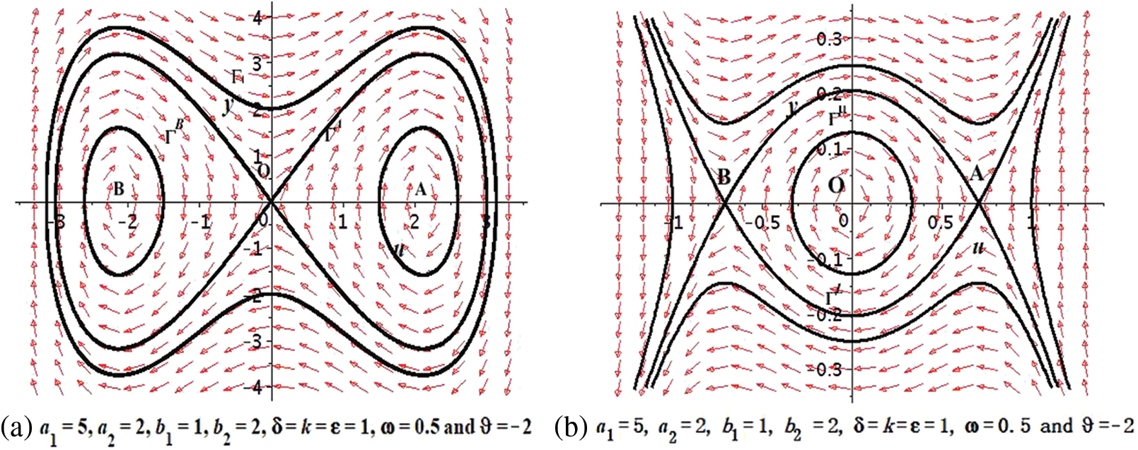
Figure 1: Bifurcation of system Eq. (5) with
(ii)
On the other hand, if
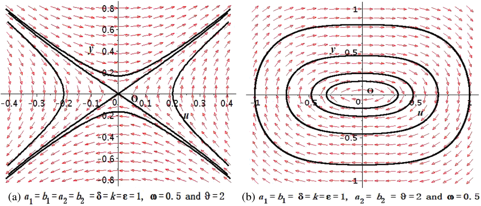
Figure 2: Bifurcation of system Eq. (5) with
Moreover, a different dynamical system can arise for
with the Hamiltonian
It has a unique critical point
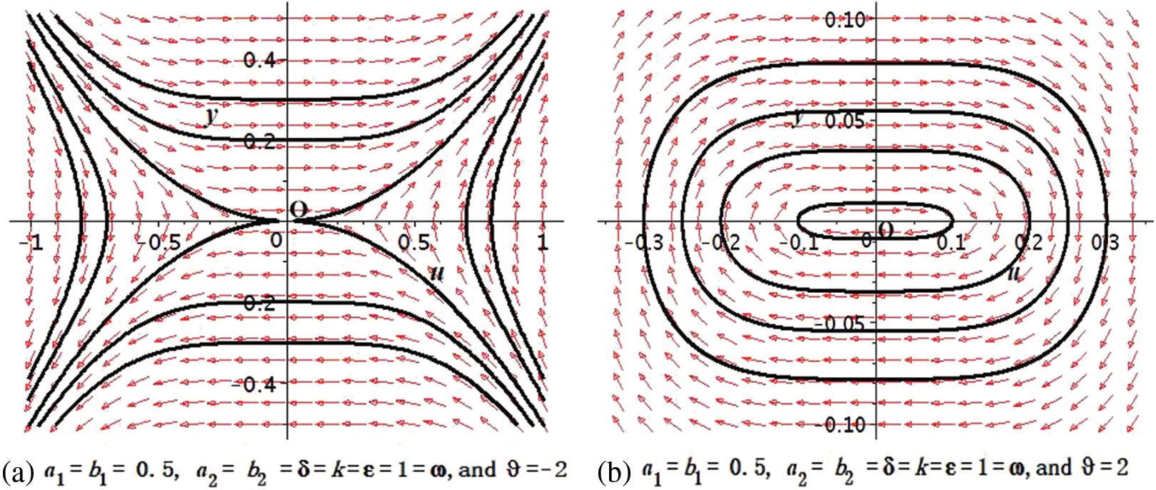
Figure 3: Bifurcation of system Eq. (5) with
2.3 Bounded Travelling Wave Solutions of BAM
This section will provide the explicit expressions of all bounded travelling wave solution of the system Eq. (5).
2.3.1 The Periodic Wave Solution
Recall the cases
where
Combining Eqs. (12) and (13), it leads to
By the direct elliptic integral and calculation, we arrive at the solution
where
where
Similarly, the periodic solution corresponding to
where
where
Again, recall the cases
where
Combining Eqs. (20) and (21), it leads to
Again by the elliptic integral and after some calculation, we arrive at the solution
where
where
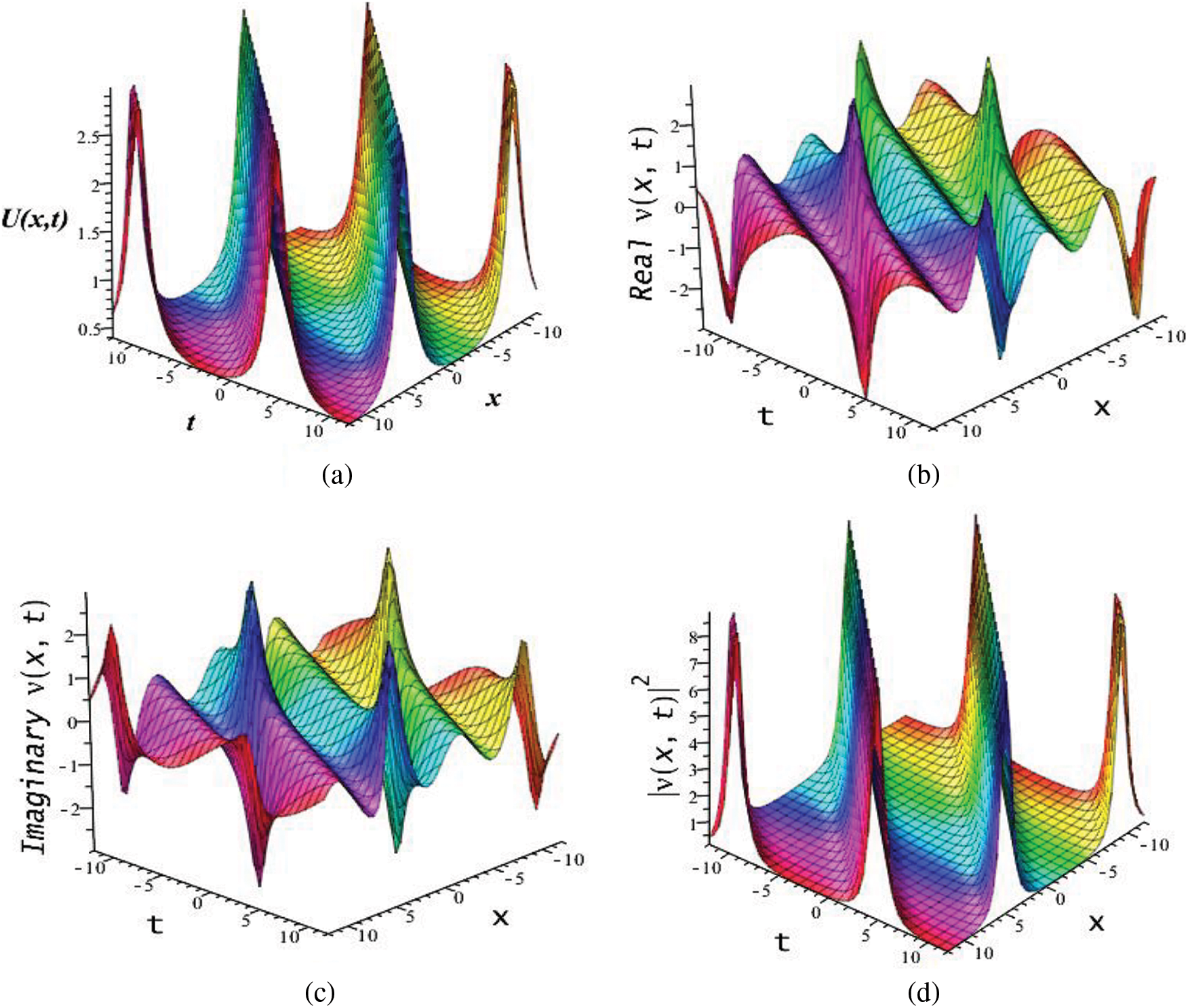
Figure 4:
2.3.2 The Solitary Wave Solutions
Using the cases
where
Applying the elliptic integral and some calculation, we arrive at the solution
The resulting solution
Similarly, let the homoclinic orbit and initial value
Through the elliptic integral and after some calculation, we arrive at the solution
The obtained solution
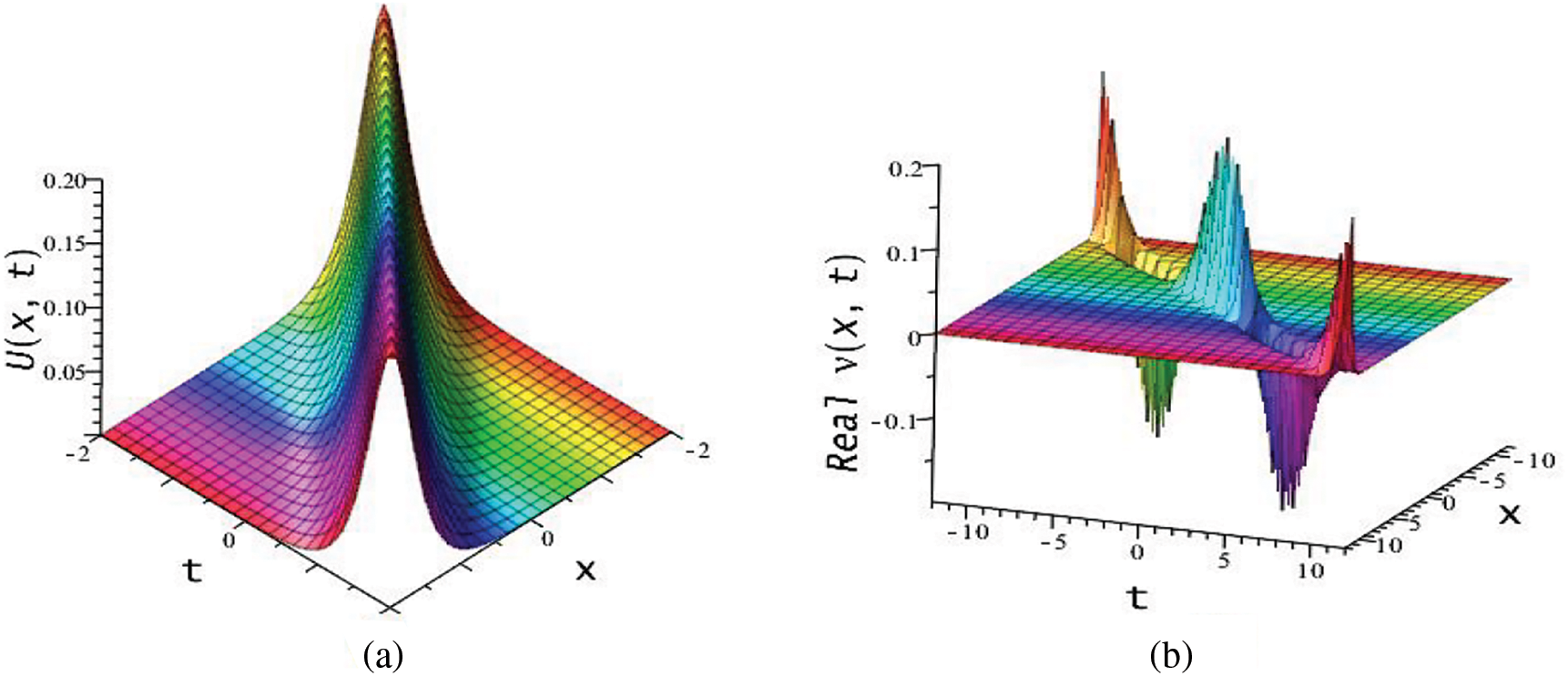
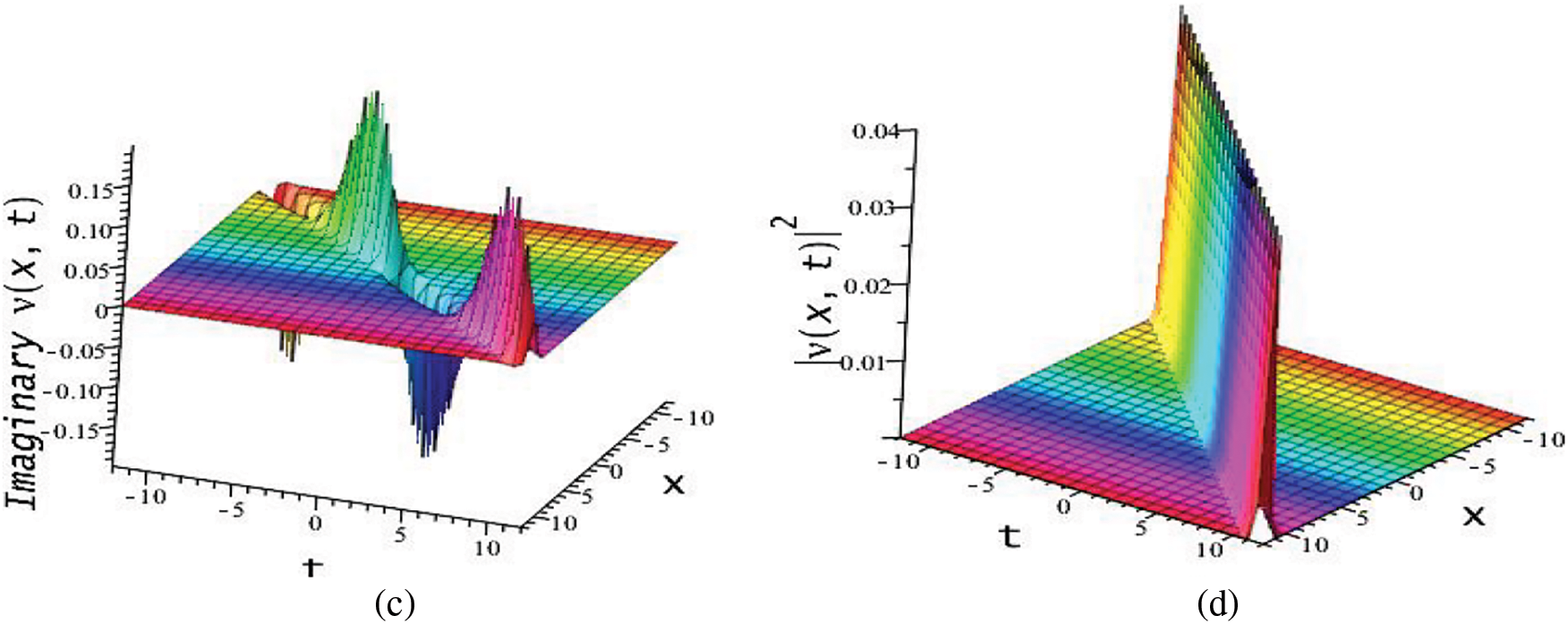
Figure 5:

Figure 6:
2.3.3 The Shock Wave Solutions
For the cases
where
and applying the elliptic integral and after some calculation, we arrive at the solution
Noting that
The resulting solution
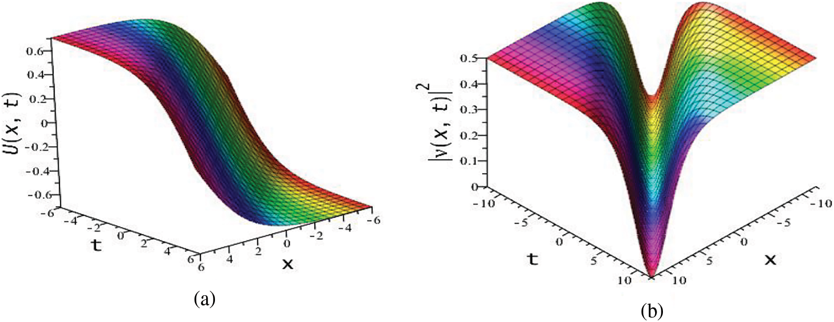
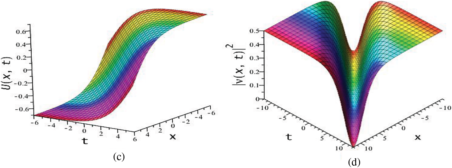
Figure 7:
2.4 Optical Soliton Solutions to BAM via the EShGEE
One considers the general form of the trail solution in the extended sinh-Gordon equation expansion approach (EShGEE) [23],
where
Due to balance principal, the value n of Eq. (35) can be obtained. The Eq. (36) has been obtained from the sinh-Gordon equation [23],
and they [23] obtained the solutions,
and
where
We now compute the balance number of Eq. (3), which leads to
Putting Eq. (40) into Eq. (3) along with Eq. (36), we obtain a polynomial of
where
Now for the Set 1, if we combine Eq. (41) with Eqs. (38)–(40), and substituting into Eq. (2), we obtain the exact soliton solutions of Eq. (1). These solutions of the model give us the optical shock wave and optical singular shock solitons,
where
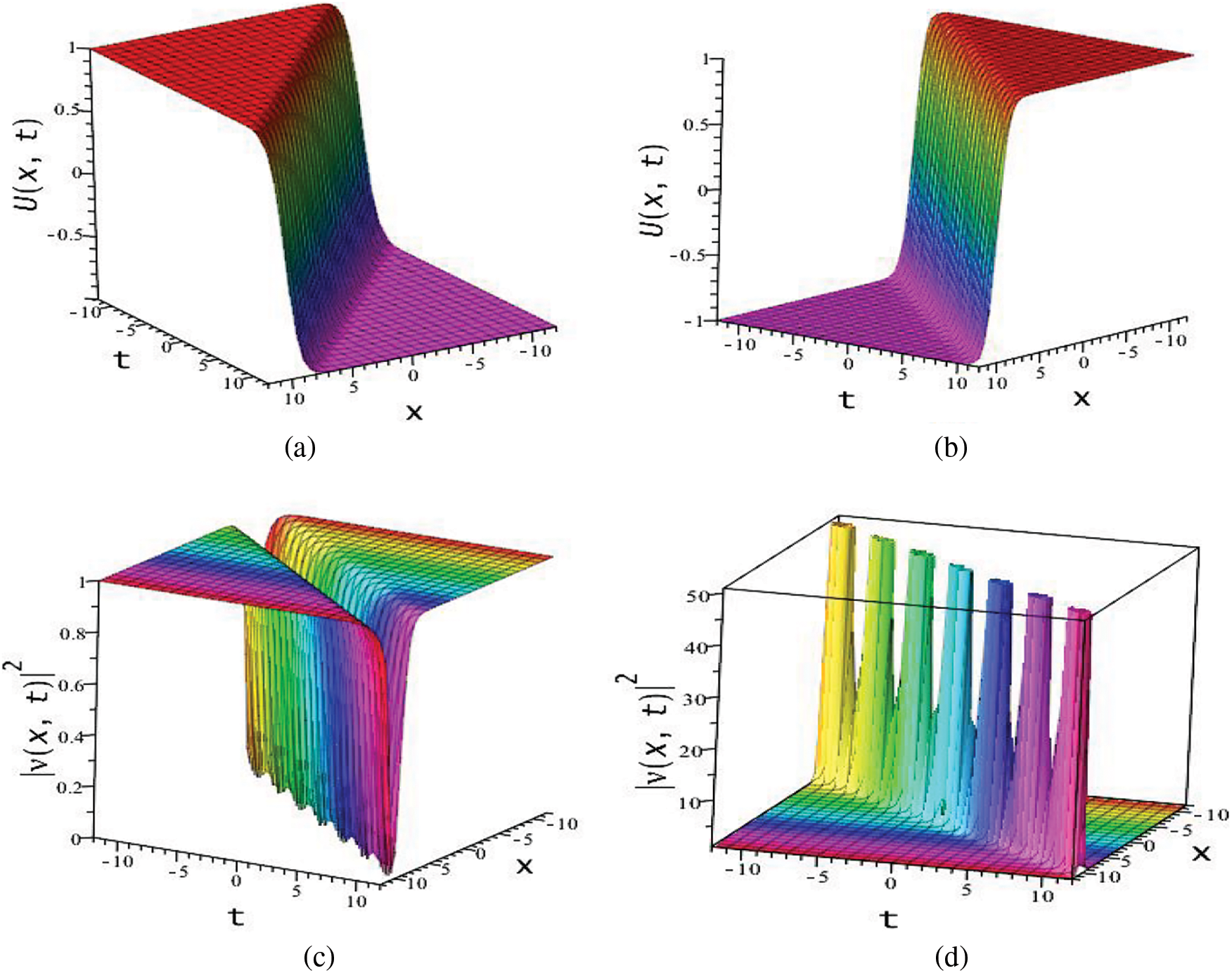
Figure 8:
Similarly, for the Set 2, if we combine Eq. (42) with Eqs. (38)–(40), and substituting into Eq. (2), we obtain the exact soliton solutions of Eq. (1). These solutions give us the combination of chirp-free bright and optical shock wave double solitons, and the combination of optical singular double solitons,
where
where
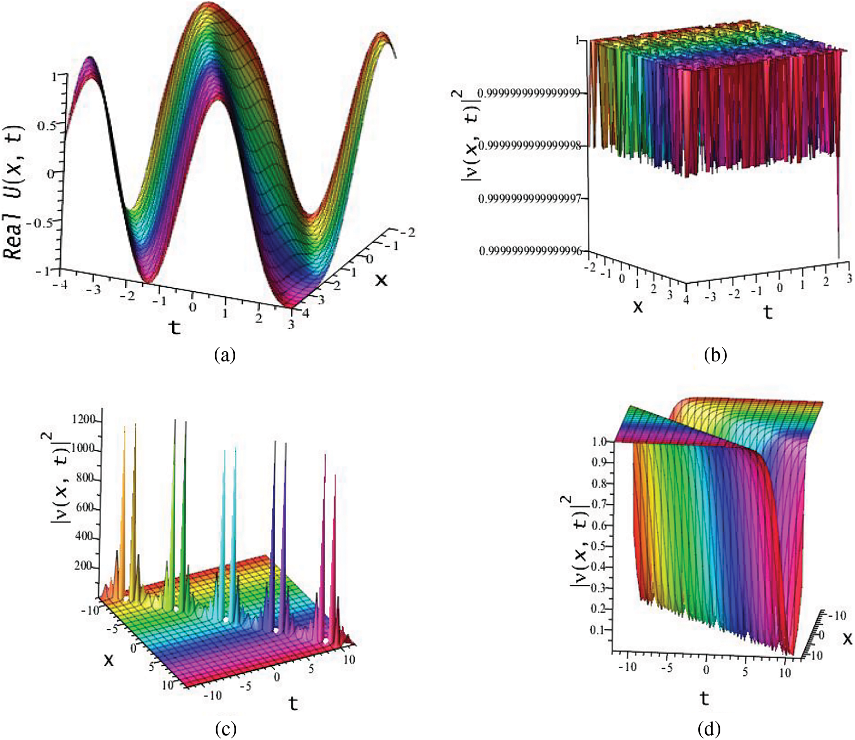
Figure 9:
2.5 Optical Soliton Solutions to the Biswas-Arshed Model via the GK Method
The GK method [30] is a unique approach to obtaining the generalized solitons and periodic rogue waves of the nonlinear evolution equations (NLEEs) [20,21]. We now consider a rational series in this method as:
where
with the solution
where h is the integral constant.
The trail solution Eq. (50) to the BAM takes the following form for the balance numbers
Putting Eq. (53) into Eq. (3) along with Eq. (51), we obtain a polynomial of
where
where
where
where
Now for the Set 1, if we combine Eq. (54) with Eq. (53) and substituting into Eq. (2), we obtain the exact soliton solutions of Eq. (1). These solutions are able to give us optical rogue wave solitons,
where
The behavior of the solution
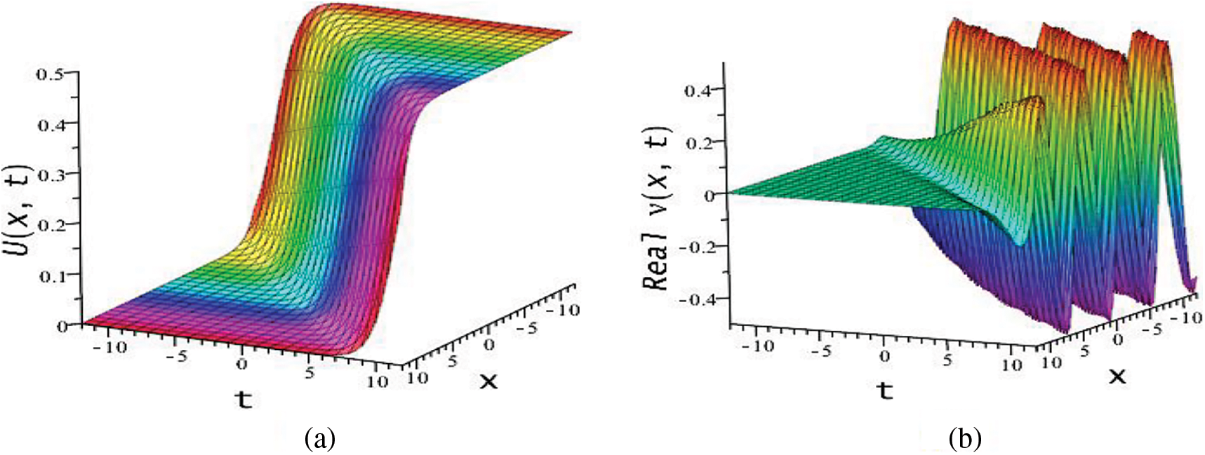
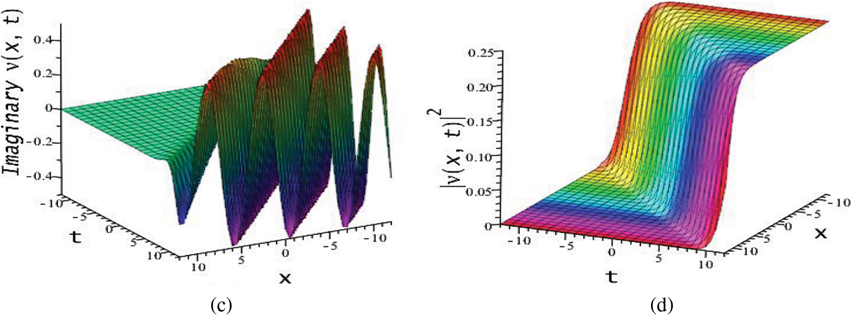
Figure 10:
Similar, for the Set 2, if we combine Eq. (55) with Eq. (53) and substituting into Eq. (2), we obtain the exact soliton solutions of Eq. (1). These solutions lead to optical rogue wave solitons,
where
where
where
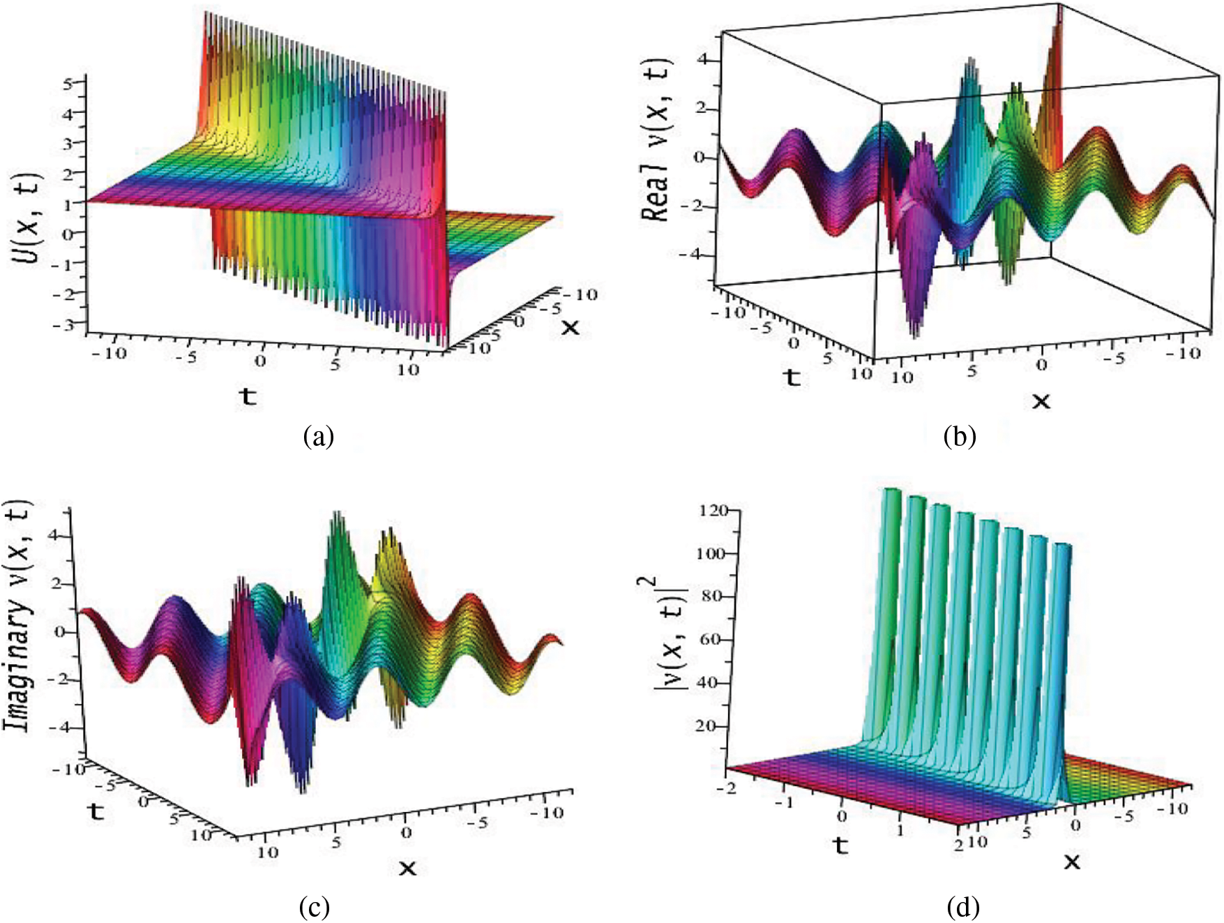
Figure 11:
This section will provide some discussions of the physical importance of the acquired results. The results of the BAM structure presented in this research have richer physical structure than earlier outcomes in the literature [11–18]. The recorded solutions are significant in the context of nonlinear dynamics, physical science, mathematical physics and the optical communication through optical fiber. We studied BAM given by Eq. (1) using bifurcation analysis, dynamical system, EShGEE and GK schemes. The bifurcation scheme provided us the evidence of the existence of various periodic wave and optical soliton solution splitting parametric areas shown in different phase portraits in Figs. 1 and 3 of the BAM. We also illustrated the physical meaning of the obtained explicit solutions 3D and contour plots that appeared in Figs. 4 and 11.
The main results of this paper are on the application of the bifurcation analysis via a dynamical system scheme and the derivation of all bounded optical wave solutions of the Biswas-Arshed model. We obtained all types of phase portraits and corresponding bounded optical shock wave, bounded solitary wave, and the bounded periodic wave solutions of the BAM by using the dynamical scheme, the extended sinh-Gordon equation expansion, and the generalized Kudryashov integral schemes. To our knowledge, these types of solitons for the Biswas-Arshed model have not been explored before [13–16,19]. All the solutions are illustrated graphically. The model could be investigated to get multi-soliton and rogue wave solutions by the other existing methods, in particular, Hirota bilinear approach [24,25] and Darboux transformation [26]. The results would be interesting to use in social media, telecommunication industries, internet zone, and many other aspects.
Acknowledgement: The authors thank to Prof. Ji-Huan He for his valuable suggestions that helped us in improving the quality and presentation of this paper.
Funding Statement: This research was supported by the Deanship of Scientific Research, Prince Sattam bin Abdulaziz University, Alkharj, Saudi Arabia, under Grant No. 2021/01/19122.
Conflicts of Interest: The authors declare that they have no conflicts of interest to report regarding the present study.
References
1. Agrawal, G. P. (2000). Nonlinear fiber optics. In: Nonlinear science at the dawn of the 21st century, pp. 195–211. Springer. [Google Scholar]
2. Haus, H. A., Wong, W. S. (1996). Solitons in optical communications. Reviews of Modern Physics, 68(2), 423. DOI 10.1103/RevModPhys.68.423. [Google Scholar] [CrossRef]
3. Zhao, L. C., Li, S. C., Ling, L. (2016). W-shaped solitons generated from a weak modulation in the Sasa-Satsuma equation. Physical Review E, 93(3), 032215. DOI 10.1103/PhysRevE.93.032215. [Google Scholar] [CrossRef]
4. Biswas, A., Yildirim, Y., Yasar, E., Zhou, Q., Moshokoa, S. P. et al. (2018). Optical solitons for lakshmanan–Porsezian–Daniel model by modified simple equation method. Optik, 160, 24–32. DOI 10.1016/j.ijleo.2018.01.100. [Google Scholar] [CrossRef]
5. Biswas, A., Yildirim, Y., Yasar, E., Triki, H., Alshomrani, A. S. et al. (2018). Optical soliton perturbation for complex Ginzburg–Landau equation with modified simple equation method. Optik, 158, 399–415. DOI 10.1016/j.ijleo.2017.12.131. [Google Scholar] [CrossRef]
6. Mirzazadeh, M., Yıldırım, Y., Yaşar, E., Triki, H., Zhou, Q. et al. (2018). Optical solitons and conservation law of Kundu–Eckhaus equation. Optik, 154, 551–557. DOI 10.1016/j.ijleo.2017.10.084. [Google Scholar] [CrossRef]
7. Biswas, A., Yildirim, Y., Yasar, E., Zhou, Q., Mahmood, M. F. et al. (2018). Optical solitons with differential group delay for coupled Fokas–Lenells equation using two integration schemes. Optik, 165, 74–86. DOI 10.1016/j.ijleo.2018.03.100. [Google Scholar] [CrossRef]
8. Biswas, A., Yıldırım, Y., Yaşar, E., Zhou, Q., Moshokoa, S. P. et al. (2018). Sub pico-second pulses in mono-mode optical fibers with Kaup–Newell equation by a couple of integration schemes. Optik, 167, 121–128. DOI 10.1016/j.ijleo.2018.04.063. [Google Scholar] [CrossRef]
9. Biswas, A., Yildirim, Y., Yasar, E., Mahmood, M. F., Alshomrani, A. S. et al. (2018). Optical soliton perturbation for Radhakrishnan–Kundu–Lakshmanan equation with a couple of integration schemes. Optik, 163, 126–136. DOI 10.1016/j.ijleo.2018.02.109. [Google Scholar] [CrossRef]
10. Biswas, A., Yildirim, Y., Yasar, E., Zhou, Q., Moshokoa, S. P. et al. (2018). Optical soliton perturbation with resonant nonlinear Schrödinger’s equation having full nonlinearity by modified simple equation method. Optik, 160, 33–43. DOI 10.1016/j.ijleo.2018.01.098. [Google Scholar] [CrossRef]
11. Biswas, A., Arshed, S. (2018). Optical solitons in presence of higher order dispersions and absence of self-phase modulation. Optik, 174, 452–459. DOI 10.1016/j.ijleo.2018.08.037. [Google Scholar] [CrossRef]
12. Yildirim, Y. (2019). Optical solitons of Biswas–Arshed equation by trial equation technique. Optik, 182, 876–883. DOI 10.1016/j.ijleo.2019.01.084. [Google Scholar] [CrossRef]
13. Yildirim, Y. (2019). Optical solitons of Biswas-Arshed equation by modified simple equation technique. Optik, 182, 986–994. DOI 10.1016/j.ijleo.2019.01.106. [Google Scholar] [CrossRef]
14. Tahir, M., Awan, A. U. (2020). Optical travelling wave solutions for the Biswas–Arshed model in kerr and non-kerr law media. Pramana, 94(1), 1–8. DOI 10.1007/s12043-019-1888-y. [Google Scholar] [CrossRef]
15. Tahir, M., Awan, A., Rehman, H. (2019). Dark and singular optical solitons to the Biswas–Arshed model with Kerr and power law nonlinearity. Optik, 185, 777–783. DOI 10.1016/j.ijleo.2019.03.108. [Google Scholar] [CrossRef]
16. Rehman, H. U., Saleem, M. S., Zubair, M., Jafar, S., Latif, I. (2019). Optical solitons with Biswas–Arshed model using mapping method. Optik, 194, 163091. DOI 10.1016/j.ijleo.2019.163091. [Google Scholar] [CrossRef]
17. Ekici, M., Sonmezoglu, A. (2019). Optical solitons with Biswas-Arshed equation by extended trial function method. Optik, 177, 13–20. DOI 10.1016/j.ijleo.2018.09.134. [Google Scholar] [CrossRef]
18. Aouadi, S., Bouzida, A., Daoui, A., Triki, H., Zhou, Q. et al. (2019). W-shaped, bright and dark solitons of Biswas–Arshed equation. Optik, 182, 227–232. DOI 10.1016/j.ijleo.2019.01.027. [Google Scholar] [CrossRef]
19. Hoque, M. F. (2020). Optical soliton solutions of the Biswas–Arshed model by the tan(Σ/2) expansion approach. Physica Scripta, 95(7), 075219. DOI 10.1088/1402-4896/ab97ce. [Google Scholar] [CrossRef]
20. Arnous, A. H., Mirzazadeh, M. (2016). Application of the generalized Kudryashov method to the Eckhaus equation. Nonlinear Analysis: Modelling and Control, 21(5), 577–586. DOI 10.15388/NA.2016.5.1. [Google Scholar] [CrossRef]
21. Ullah, M. S., Ali, M. Z., Rahman, Z. (2019). Novel exact solitary wave solutions for the time fractional generalized Hirota–Satsuma coupled kdV model through the generalized Kudryshov method. Contemporary Mathematics, 1, 25–32. DOI 10.37256/cm.11201936.25-33. [Google Scholar] [CrossRef]
22. Fu, Z., Liu, S., Liu, S. (2006). Exact jacobian elliptic function solutions to sinh-Gordon equation. Communications in Theoretical Physics, 45(1), 55. DOI 10.1088/0253-6102/45/1/010. [Google Scholar] [CrossRef]
23. Yang, X., Tang, J. (2008). Travelling wave solutions for Konopelchenko–Dubrovsky equation using an extended sinh-gordon equation expansion method. Communications in Theoretical Physics, 50(5), 1047. DOI 10.1088/0253-6102/50/5/06. [Google Scholar] [CrossRef]
24. Harun, R., Ma, W. (2018). Dynamics of mixed lump-solitary waves of an extended (2+1)-dimensional shallow water wave model. Physics Letters A, 382(45), 3262–3268. DOI 10.1016/j.physleta.2018.09.019. [Google Scholar] [CrossRef]
25. Wang, X. B., Tian, S. F., Qin, C. Y., Zhang, T. T. (2017). Characteristics of the solitary waves and rogue waves with interaction phenomena in a generalized (3+1)-dimensional Kadomtsev–Petviashvili equation. Applied Mathematics Letters, 72, 58–64. DOI 10.1016/j.aml.2017.04.009. [Google Scholar] [CrossRef]
26. Bagrov, V. G., Samsonov, B. F. (1997). Darboux transformation and elementary exact solutions of the Schrödinger equation. Pramana, 49(6), 563–580. DOI 10.1007/BF02848330. [Google Scholar] [CrossRef]
27. Nemytskii, V. V. (2015). Qualitative theory of differential equations. USA: Princeton University Press. [Google Scholar]
28. He, J. H., Hou, W. F., He, C. H., Saeed, T., Hayat, T. (2021). Variational approach to fractal solitary waves. Fractals, 29(7), 2150199. DOI 10.1142/S0218348X21501991. [Google Scholar] [CrossRef]
29. He, J. H., He, C. H., Saeed, T. (2021). A fractal modification of Chen–Lee–Liu equation and its fractal variational principle. International Journal of Modern Physics B, 35(21), 2150214. DOI 10.1142/S0217979221502143. [Google Scholar] [CrossRef]
30. Ullah, N., Asjad, M. I., Iqbal, A., Rehman, H. U., Hassan, A. et al. (2021). Analysis of optical solitons solutions of two nonlinear models using analytical technique. AIMS Mathematics, 6(12), 13258–13271. DOI 10.3934/math.2021767. [Google Scholar] [CrossRef]
Cite This Article
 Copyright © 2023 The Author(s). Published by Tech Science Press.
This work is licensed under a Creative Commons Attribution 4.0 International License , which permits unrestricted use, distribution, and reproduction in any medium, provided the original work is properly cited.
 Downloads
 Citation Tools