DOI:10.32604/csse.2021.013843
| Computer Systems Science & Engineering DOI:10.32604/csse.2021.013843 | |
| Article |
Automatic Channel Detection Using DNN on 2D Seismic Data
1Imam Abdulrahman Bin Faisal University, College of Computer Science and Information Technology, Dammam, 34212, Saudi Arabia
2Saudi Aramco Oil Company, EXPEC-II, Dhahran, Saudi Arabia
*Corresponding Author: Ilyas A. Salih. Email: ilyasbinsalih@gmail.com
Received: 30 August 2020; Accepted: 29 October 2020
Abstract: Geologists interpret seismic data to understand subsurface properties and subsequently to locate underground hydrocarbon resources. Channels are among the most important geological features interpreters analyze to locate petroleum reservoirs. However, manual channel picking is both time consuming and tedious. Moreover, similar to any other process dependent on human intervention, manual channel picking is error prone and inconsistent. To address these issues, automatic channel detection is both necessary and important for efficient and accurate seismic interpretation. Modern systems make use of real-time image processing techniques for different tasks. Automatic channel detection is a combination of different mathematical methods in digital image processing that can identify streaks within the images called channels that are important to the oil companies. In this paper, we propose an innovative automatic channel detection algorithm based on machine learning techniques. The new algorithm can identify channels in seismic data/images fully automatically and tremendously increases the efficiency and accuracy of the interpretation process. The algorithm uses deep neural network to train the classifier with both the channel and non-channel patches. We provide a field data example to demonstrate the performance of the new algorithm. The training phase gave a maximum accuracy of 84.6% for the classifier and it performed even better in the testing phase, giving a maximum accuracy of 90%.
Keywords: Deep neural networks; deep learning; channel detection; image processing; two-dimensional seismic data
Processing and interpreting seismic data are important for most present-day oil and gas exploration. Seismic data contain various information about the subsurface, such as structure and lithology [1]. Underground geological features hold particularly important information that could affect drilling decisions. Channels are a significant geological feature that can be considered as either potential paths for petroleum migration or drilling hazards; in either case, channels should be detected in seismic data before the drilling process commences [2].
In geology, a channel is a landform consisting of thick lines that are covered with a narrow area of water underground. They are formed through a complex process. Since channel locations are surrounded by beds of sedimentary rocks, it is hard to detect some channels, and they may well even go unnoticed. In the petroleum field, buried underground channels are very profitable for oil companies because they can contain tons of oil and gas that can be extracted. Channel behavior can also change faster than other seismic data features, and sometimes they vanish over time, making channel prediction using geophysical data harder and more challenging [3].
Previously, channel detection via seismic imaging was performed manually. Manual channel picking is both time consuming and tedious. Moreover, similar to any other process dependent on human intervention, manual channel picking is error prone and inconsistent. Therefore, this paper proposes an automatic machine learning algorithm to detect channels in 2D seismic data. This new algorithm focuses on automating channel detection and employs a machine learning algorithm—the deep neural network (DNN)—to identify channels in seismic images. Research done using the classical approach and machine learning approach for detecting channels in seismic data are discussed.
The remainder of this paper is organized as follows. Section 2 contains a review of related literature. Section 3 contains the proposed method. Section 4 demonstrates a field data example. Section 5 presents the results and discussion. Finally, the conclusion is given in Section 6.
In this section, several studies are explored to understand the previous studies for channel detection on seismic data. Two main categories have been considered in this paper, the statistical approaches and the machine learning approaches.
2.1 Classical/Image-Processing Approaches
Shearlet transformation has applications in numerous areas including feature extraction, image fusion, geophysical noise attenuation, and seismic feature detection. Shearlet transformation outperforms both Sobel and Canny methods in detecting channels. Channels in seismic images can be regarded as edges [4]. In Karbalaali et al. [5], the authors used an algorithm that works by breaking the input data into various scales and directions via multiplication of Shearlet filters in the frequency domain. Then, they determined the edge candidates by finding the local maxima coefficients of Shearlet at the finest scale. At each pixel of each cone, they maximized the Shearlet coefficient associated with that cone by finding its maximum value. Cones are formed by partitioning the Fourier domain into four parts, with each cone having a finite range in which the shearing variable is allowed to vary in cone-adapted Shearlet transformation. After that, a threshold scheme needs to be applied to get the binary image pixels classified into edge and non-edge based on the Shearlet coefficient’s local maxima. Finally, the resulting image will fall into two classes, with edge and none-edge labels. The resulting image may require enhancement by applying morphological thinning, which removes selected foreground pixels from the binary image. Foreground pixels are those that do not match with the underlying pixel values or background pixels in morphological operations. Thinning is used in this algorithm to reduce the edges on the borders by applying a threshold method and removing points that share multiple foregrounds.
In Mardan et al. [6], the authors implemented channel detection using a K-means algorithm and support vector machine (SVM). The dataset used for the experimental implementation was provided by the National Iranian Oil Company (NIOC). The researchers approached the channel detection task as a classification problem. The K-means method they used classified channels into three clusters as the output of this algorithm. Then, SVM was fed with the output of the K-means algorithm as input seeds for the SVM models. With training samples, the authors achieved 94.7% accuracy.
In Cao et al. [7], the authors used a color-blending visualization approach depend on different color models with seismic attribute combinations for the purpose of detecting subsurface channels. The three types of color models used were the RGB (red, green, blue) model, the CMY (cyan, magenta, yellow) model, and the HSV (hue, saturation, value) model. For forecasting subsurface channels, sensitive seismic attribute volumes were measured from the basic seismic data where only three categories of attributes are combined together in three-dimensional space. According to the authors, the RGB and CMY models gave better resolution compared to the HSV model, and the color blending in the RGB model was more contrasting than that of the CMY model in terms of the background of the seismic images.
In Mathewson et al. [8], the authors used steerable pyramid filters to splitting the seismic image based on the scale and orientation to detect channels in the images. Features were selected and determined based on dimensionality and directions resulted from the partitioned image. Then, the authors implemented steerable pyramids in 2D and 3D to enhance the image features, and by doing so, the authors were able to enhance the channels on synthetic seismic images.
2.2 Machine Learning Approaches
Machine learning (ML) methods can predict and estimate the pattern and relationship that exists among the samples in the dataset. Recently, ML methods have become increasingly popular within the scientific community. In ML, seismic data interpolation can be viewed as a regression problem for continuous output.
In Krasnov et al. [9], they proposed using ANN model to detect channels based on features extracted from seismic cubes. The dataset holds RGB maps obtained from geological units in a Z axes seismic data range where the boundaries of such selected range determined by using secant surfaces. To reflect the coordinates of the selected range and to determine its frequencies, they applied continuous wavelet transformation (CWT). Then, the created dataset used to train the ML model where they manually performed the classification of the RGB maps within the dataset to highlight the channels. Due to the huge number of maps, they used a subset of the dataset consists of about 50 maps for each type (with channel and without channel). The authors used the Xception DNN along with ImageNet dataset. Xception is designed to classify 1000 classes of objects from ImageNet. There are no geological objects in the dataset; therefore, the authors used the knowledge transfer method. The main idea is to use only a part of the trained DNN layers, develop one’s own layers, and retrain the DNN with data from the channel domain, that is, the images from mini RGB maps. An image close-up method was then later used to manually increase the dataset. The authors did not mention anything about their accuracy but gave other performance metrics like precision, recall, and F1-score, with average values of 91%, 88%, and 89%, respectively.
Perters et al. [10] introduced Neural nets framework for geophysicists wherein they can perform modeling and inversion. Further, they described comparisons of DNN and other geophysical inverse problems. It also includes demonstration to explain their helpfulness in problem solving of lithology, interpolation between wells, horizon tracing, and separation of seismic images.
Ma et al. [11] conducted an intense study of around 200 recent publications on applications of Deep learning algorithms in remote sensing image analysis. Their study investigated the meta-analysis in the beginning for analyzing the status of remote sensing of targets and later modeling, image spatial resolution, area type and accuracy of classification was accomplished by the application of Deep learning methods. In addition, the utilization of Deep learning in image combination, image registration, scene sorting, object recognition, land use and land cover classification, segmentation, and object analysis were reviewed.
Zeng et al. [12], demonstrated the benefits of CNN for classification to define salt body with high precision. For accurate prediction, they have combined Exponential Linear Units, activation function, the Lovasz-Softmax loss function, and stratified K-fold cross-validation in their research. Based on the literature review and due to the promising features of DNN, we chose DNN as a model for our proposed method as shown in the next sections.
In this paper, a method based on DNNs is proposed to detect channels in 2D seismic data. Channels can be characterized as having unique spatial signatures and long axis direction extension resulting in local linearity, which makes it a bit easier to be detected. The DNN consists of three convolution layers, every one of which is followed by a rectified linear unit (ReLU) layer for nonlinear activation. A ReLU layer accomplishes a threshold operation on each and every parameter of the input value and sets negative values to zero [13]. The ReLU function is shown as Eq. (1):

Two max pooling layers are sandwiched between the convolution layers to improve the computational time required to train. A max pooling layer performs a down-sampling operation by dividing the input into rectangular pooling regions and computing the maximum value in each region [14]. It also has a fully connected layer through which the learning process takes place, as shown in Fig. 1. The fully connected layer has a dropout layer to minimize the effect of overfitting while training the model after the convolution process. Finally, in the output layer, a Softmax activation function classifies the patches into channel or non-channel patches. It is the output unit activation function after the last fully connected layer for multiclass classification problems [15]. A Softmax function in use by the Softmax layer can be expressed as shown in Eq. (2):

where xi is the ith dimension output and N is the number of classes [16]. Layers used in the DNN are described in Tab. 1.
Table 1: Deep neural network layer details
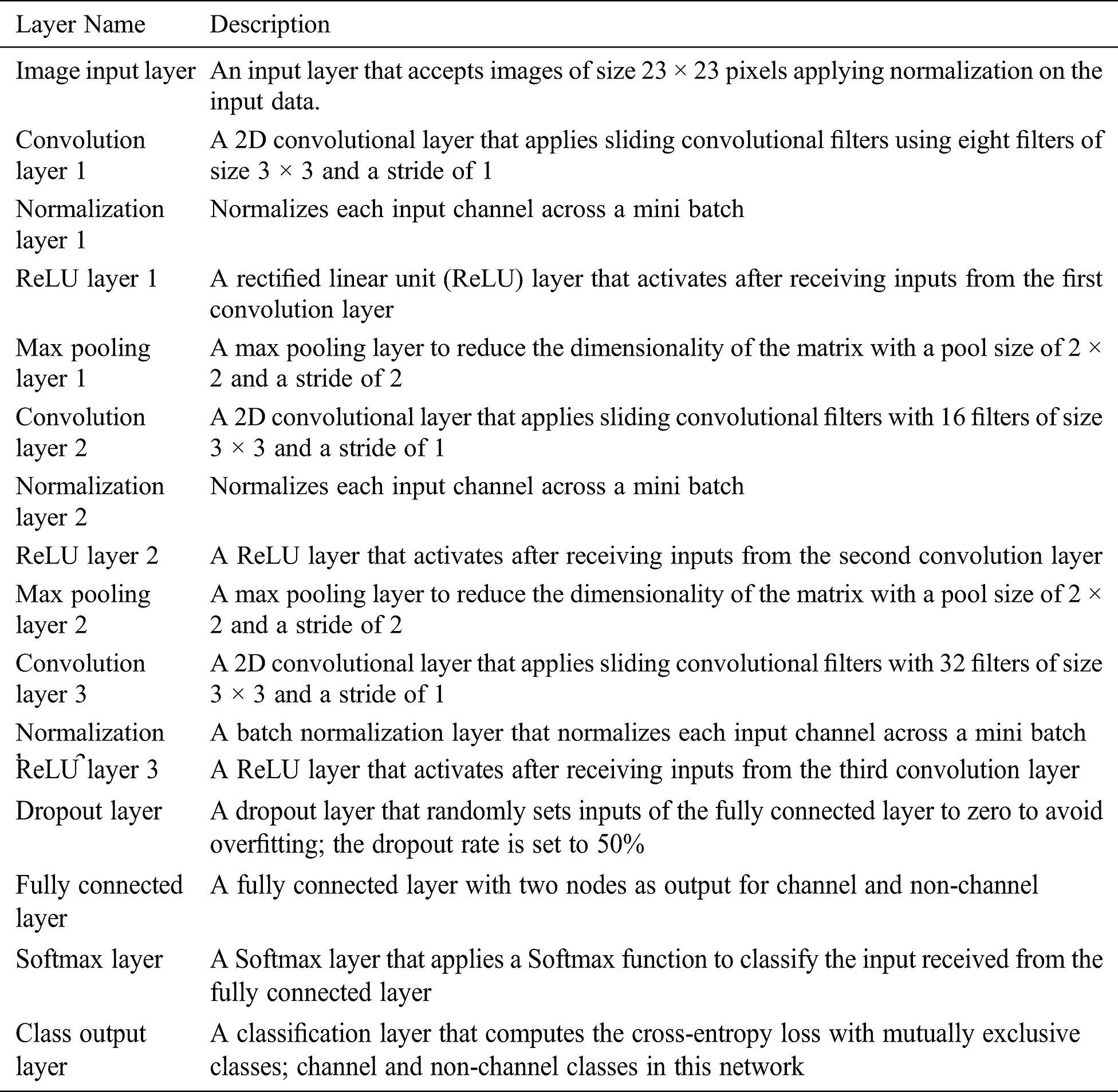
The proposed DNN has 16 layers, including the input and output layers as shown in Fig. 1. The layers are divided into three parts: input layer, middle layers or hidden layers, and output layer. The input layer takes grayscale images with dimensions 23 × 23. The dimensions are set to this specific value because of the fixed size of the patches. The middle layers have three convolution layers with a batch normalization layer and ReLU activation layers. The first convolution layer applies sliding convolutional filters to the input with eight filters of size 3 × 3 and stride 1. Since this was the smallest, we could go to detect a channel’s features in a given area of the picture we went by 3 × 3 size filter and a stride of 1 to to not miss any feature from the image’s patches. The eight filters will extract the channel features from the patched images that is later fed to the network. A batch normalization layer is used after it to normalize each input channel across a mini batch. After the normalization and activation layers, a max pooling layer is added to decrease the computational power required to process the data through reducing dimensionality and extracting dominant features. The layer has a size of 2 × 2 and stride 2. The second convolution layer applies sliding convolutional filters to the input with 16 filters of size 3 × 3 and stride 1 as well to extract the features from the channel patches and non-channel patches. A batch normalization layer, ReLU activation layer, and max pooling layer are added after the convolution layer like for the first convolution layer. The third convolution layer applies sliding convolutional filters to the input with 32 filters of size 3 × 3 and stride 1, followed by a batch normalization layer and ReLU layer for feature extraction. After the convolution layers, a dropout layer is added before the fully connected layer. The dropout layer randomly sets input elements to zero and is used to prevent overfitting during the training process in the fully connected layer. The fully connected layer has an output size of 2 (i.e., channel or non-channel). The last layer of the DNN is the output layer, which computes the cross-entropy loss with mutually exclusive classes, which then classifies a patch as channel or non-channel.

Figure 1: DNN architecture
The implementation of the proposed method comprises three stages: (1) A patching process, in which the images are divided into patches; (2) A training process, in which the patches are used to train the developed DNNs; and (3) An output process, in which the trained model is used to trace the channel on a given 2D seismic image. All the experiments were carried out in MATLAB 2018a. The overall methodology is depicted in Fig. 2.

Figure 2: Overall architecture of the implementation
The sample dataset is a 3D seismic image cube that consists of 75 depth slices. Some of the slices contain no channels or unclear channels and are labeled as low-quality slices, while the slices that have clear channels in them are labeled as high-quality slices. A total of four high-quality slices are chosen to train the network, as shown in Tab. 2, with the number of channel and non-channel patches in them after the patching process.

Each slice needs to be divided into 23 × 23-pixel patches, which are then fed to the DNN to be trained. The total number of patches for all four images is 1,326,384. Before the patching begins, padding is added to both the channel image and the ground truth image. Padding ensures that none of the pixels are lost, thus saving all the features that are present in the image to be recognized by the network. Fig. 3 illustrates the patching process. The patching process works by dividing the ground truth image and the real image into patches and then checking each of the ground truth patch’s pixel values using a zero-centering technique. If the pixel value is found to be less than the assigned threshold value, it is classified as a patch with channels, and the channel image’s patch matching with that of the ground truth’s patch is added to the “channel” folder; otherwise, it is added to the “non-channel” folder.
At the completion of the patching process, the patches are used as input to the DNN’s input layer. The input layer has dimensions of 23 × 23 × 1, as the patches are of these exact dimensions. Once the training process begins, the weights are adjusted to differentiate the channel patches from the ones that do not have channels to train the proposed model. The training process using all the patches takes approximately 3 days on a good PC.

Figure 3: Patching process
The output process works by patching the new channel image into the specified 23 × 23-pixel patches. Each patch is then passed through the trained network to classify it as a channel or non-channel patch. If the network identifies the patch as a channel patch, it changes the pixel value of that patch’s location on the output image to 0, resulting in a black spot, and if the patch is not a channel patch, the pixel value is set to 1, resulting in a white spot on the output image. The process is repeated until the whole image is traversed using the 23 × 23-pixel patch. Thus, an output image is obtained showing traces of channels.
The network gave a maximum accuracy of 84.6% in the training phase and a maximum accuracy of 90% in the testing phase. The accuracy obtained in training is after experimenting with different parameters and training options. This includes experimenting the size of the filters, the number of the filters, batches sizes, and learning rates parameters. The confusion matrix from the training phase is shown in Fig. 4 below. It shows all the patches that were classified correctly and incorrectly including the true positives and negatives during the training phase. The model classified 2.1% of the total dataset as channel patches and 82.5% of the dataset as non-channel patches. Due to the similar features in some patches, the model also misclassified 14.7% of the non-channel patches as channel patches but only 0.7% of the channel patches were misclassified as non-channel patches due to channel patches having distinct features.
The network model gives better accuracy in training using LearnRateSchedule as piecewise in the training options but gives bad results during the testing phase. On the other hand, using LearnRateSchedule as constant gives lesser accuracy compared to piecewise but is more accurate in the testing phase. Fig. 5 illustrates in detail the training and testing results.
The trained network performs well and output satisfied results, as depicted in Figs. 6–8. The network traced channel patches better than the provided ground truth images for each channel image. For example, the output on the right in Fig. 6 shows the detected channels related to 181th Seismic Slice presented on the left side of the same figure, and clearly it highlights the channel as expected with minimum distortion and noise. The obtained output in Fig. 6 has been shown to an expert at ARAMCO resulting in high satisfaction. Similarly, Figs. 7 and 8 shows the channel images used for testing, and its corresponding output that show the channels detected using the developed DNN with the channels obtained and marked with arrows for comparison purposes.

Figure 4: Confusion Matrix for Training Phase

Figure 5: Constant and piecewise training option results for training and testing phases
It can be clearly seen from the above charts that the piecewise training option gave promising results in the training results but failed to give a much better result during testing. In contrast, the constant training option gave good accuracy during training and even better accuracy during the testing phase. The constant training option took considerably more time to train the network as compared to the piecewise option but gave a much promising result at the end.

Figure 6: 181th seismic slice (left) and channels detected (right) using the developed DNN

Figure 7: 189th seismic slice (left) and channels detected (right) using the developed DNN

Figure 8: Seismic slice from a different dataset (left) and channels detected on the slice (right) using the developed DNN
A deep learning–based channel detection algorithm was proposed, implemented, and tested on 2D field seismic data. The network training process took almost 3 days and gave good results using the constant training option compared to the piecewise training option. The model trained using constant training gave exceptionally good results in the testing phase. The images tested using the trained model gave better results than the ground truth image provided to train the network. The testing phase also showed an increase of 9% in accuracy using the constant training option, thus giving the clear channels on the tested images shown in the results.
Acknowledgement: The authors thank everyone who provided us with insight and expertise from Saudi Aramco, which in turn helped us greatly in our research work. Also, the authors thank Imam Abdulrahman Bin Faisal University for the sponsorship of this search. We express our indebtedness, gratitude, and thanks for those who guided, encouraged, and advised us throughout the course of this research.
Funding Statement: The author(s) received no specific funding for this study.
Conflicts of Interest: The authors declare that they have no conflicts of interest to report regarding the present study.
1. Seismic Testing FAQ. Elbert County. [Online]. Available: http://www.elbertcounty-co.gov/docs/Seismic_Testing_FAQ.pdf. [Google Scholar]
2. H. Karbalaali, A. Javaherian, S. Torabi, S. Dahlke, N.Keshavarz et al. (2017). , “Channel edge detection based on 2D compactly-supported shearlets, an application to a channelized seismic data in south Caspian Sea,” in Proc. of the 79th EAGE Conf. and Exhibition 2017, Paris, France, pp. 1–5. [Google Scholar]
3. J. Cao, Y. Yue, K. Zhang, J. Yang and X. Zhang. (2015). “Subsurface channel detection using color blending of seismic attribute volumes,” International Journal of Signal Processing, Image Processing and Pattern Recognition, vol. 8, no. 12, pp. 157–170. [Google Scholar]
4. H. Karbalaali, A. Javaherian, S. Dahlke, R. Reisenhofer and S. Torabi. (2018). “Seismic channel edge detection using 3D shearlets-A study on synthetic and real channelised 3D seismic data,” Geophysical Prospecting, vol. 66, no. 7, pp. 1272–1289. [Google Scholar]
5. H. Karbalaali, A. Javaherian, S. Dahlke and S. Torabi. (2017). “Channel boundary detection based on 2D shearlet transformation: An application to the seismic data in the South Caspian Sea,” Journal of Applied Geophysics, vol. 146, pp. 67–79. [Google Scholar]
6. A. Mardan, A. Javaherian and M. Mirzakhanian. (2017). “Channel characterization using support vector machine,” in 79th EAGE Conf. and Exhibition 2017–Workshops, Paris, France, pp. 45–48. [Google Scholar]
7. J. Cao, Y. Yue, K. Zhang, J. Yang and X. Zhang. (2015). “Subsurface channel detection using color blending of seismic attribute volumes,” International Journal of Signal Processing, Image Processing and Pattern Recognition, vol. 8, no. 12, pp. 157–170. [Google Scholar]
8. J. Mathewson and D. Hale. (2008). “Detection of channels in seismic images using the steerable pyramid,” SEG Technical Program Expanded Abstracts 2008, pp. 859–863. [Google Scholar]
9. F. V. Krasnov, A. V. Butorin and A. N. Sitnikov. (2018). “Automatic detection of channels in seismic images via deep learning neural networks,” Business Informatics, vol. 44, no. 2, pp. 7–16. [Google Scholar]
10. B. Peters, E. Haber and J. Granek. (2019). “Neural networks for geophysicists and their application to seismic data interpretation,” Leading Edge, vol. 38, no. 7, pp. 498–576. [Google Scholar]
11. L. Ma, Y. Liu, X. Zhang, Y. Ye, G. Yin et al. (2019). , “Deep learning in remote sensing applications: A meta-analysis and review,” ISPRS Journal of Photogrammetry and Remote Sensing, vol. 152, pp. 166–177. [Google Scholar]
12. Y. Zeng, K. Jiang and J. Chen. (2019). “Automatic seismic salt interpretation with deep convolutional neural networks,” in Proc. of the 2019 3rd Int. Conf. on Information System and Data Mining, New York, NY, USA, pp. 16–20. [Google Scholar]
13. Rectified linear unit (ReLU) layer. MathWorks. [Online]. Available: https://www.mathworks.com/help/deeplearning/ref/nnet.cnn.layer.relulayer.html. [Google Scholar]
14. Max pooling 2D layer. MathWorks. [Online]. Available: https://www.mathworks.com/help/deeplearning/ref/nnet.cnn.layer.maxpooling2dlayer.html. [Google Scholar]
15. Softmax layer. MathWorks. [Online]. Available: https://www.mathworks.com/help/deeplearning/ref/nnet.cnn.layer.softmaxlayer.html. [Google Scholar]
16. Y. Wu, J. Li, Y. Kong and Y. Fu. (2016). , “Deep convolutional neural network with independent softmax for large scale face recognition,” in Proc. of the 24th ACM Int. Conf. on Multimedia, New York, NY, USA, pp. 1063–1067. [Google Scholar]
 | This work is licensed under a Creative Commons Attribution 4.0 International License, which permits unrestricted use, distribution, and reproduction in any medium, provided the original work is properly cited. |