Computer Systems Science & Engineering DOI:10.32604/csse.2021.014100
Article

Effective Latent Representation for Prediction of Remaining Useful Life

Qihang Wang and Gang Wu*

Shanghai Jiaotong University, Shanghai, 200240, China
*Corresponding Author: Gang Wu. Email: dr.wugang@sjtu.edu.cn
Received: 31 August 2020; Accepted: 19 October 2020

Abstract: AI approaches have been introduced to predict the remaining useful life (RUL) of a machine in modern industrial areas. To apply them well, challenges regarding the high dimension of the data space and noisy data should be met to improve model efficiency and accuracy. In this study, we propose an end-to-end model, termed ACB, for RUL predictions; it combines an autoencoder, convolutional neural network (CNN), and bidirectional long short-term memory. A new penalized root mean square error loss function is included to avoid an overestimation of the RUL. With the CNN-based autoencoder, a high-dimensional data space can be mapped into a lower-dimensional latent space, and the noisy data can be greatly reduced. We compared ACB with five state-of-the-art models on the Commercial Modular Aero-Propulsion System Simulation dataset. Our model achieved the lowest score value on all four sub-datasets. The robustness of our model to noise is also supported by the experiments.

Keywords: Deep learning; predictive maintenance; remaining useful life

1  Introduction

Prognostic and health management (PHM) [1] is a basic requirement for condition-based maintenance in many fields where the safety, reliability, and availability of systems are considered mission-critical [2]. Remaining useful life (RUL) predictions are the jewel in the crown. The RUL of a machine is defined as the length, from the present to the end, of the useful life of one component [3]. It is necessary and valuable to predict precise RULs in many industrial areas, such as in manufacturing, aerospace, shipping, and mining, due to the fact that precise RUL predictions ensure smooth component replacements, reduce maintenance costs, and avoid permanent damage.

According to a recent review [4], the approaches of RUL predictions can be divided into 4 categories based on their basic techniques and methodologies, i.e., physics model-based approaches, statistical model-based approaches, artificial intelligence (AI) approaches, and hybrid approaches. Among them, AI approaches are highly thought of and particularly appealing due to their accuracy, robustness, and scalability in complex engineering systems [5].

Recurrent neural networks (RNNs) and convolutional neural networks (CNNs) are popular AI models in RUL predictions. The RNN is designed to model sequence data of varying lengths, which is very suitable for RUL predictions. Valine RNN has been used as well to predict the RUL [6]. However, the gradient in valine RNN tends to either explode or vanish over long time steps in the back-propagation stage, which is known as the long-term time dependence problem [7]. Long short-term memory (LSTM), one of the variants of valine RNN, has been introduced to solve this problem. Unidirectional LSTM and bidirectional LSTM (Bi-LSTM) have also been used to predict the RUL [5,8]. Besides, the CNN has shown remarkable success in various applications, especially in computer vision [9]. For example, the CNN and RNN were successfully combined in RUL predictions [10,11]. The combination of the CNN and RNN enabled the model to discover potential interrelationships and features that could significantly improve the capability of generalization.

However, directly feeding raw sensor data into those AI models might lead to poor performance because of noisy sensor data that can be contaminated due to sensor failures. Moreover, some feature engineering methods might generate a huge number of features, such as the sliding window method, which is widely used in RUL predictions. The number of features equals the size of the sliding window multiplied by the number of sensors. In real applications, one could end up with thousands of features due to the large number of sensors and complex operation conditions.

To tackle these challenges, some methods of denoising and dimensionality reduction are used. For example, Bai et al. [12] applied different kernel sizes for the CNN. Two-dimensional (2D) convolutions can extract features from several different sensors simultaneously, which sometimes reduces noisy data in the result. In contrast, one-dimensional (1D) convolutions can only function in the temporal dimension of a given sensor, and they extract features without any interference from the other sensor values. Another denoising solution is to reduce the dimensions of the data. Utilizing an autoencoder is popular in dimensionality reduction. The autoencoder is employed to learn a low-dimensional latent space for a set of high-dimensional input data. To incorporate richer representation of information in latent space, the reconstruction loss is computed between the original data (the input of encoders) and the generated data (the output of decoders). For example, an RNN-based autoencoder was built to obtain the health index for RUL predictions [13]. It maintained a set of intermediate embeddings and a set of health indices, which were computed based on normal behavior instances. Similarities were computed from the results of those sets and the test instance to predict the RUL. This method was also applied to the bidirectional RNN autoencoder to convert high-dimensional sensor data into a low-dimension embedding [14].

In practice, these methods still have some problems. Reference [13] maintained two sets and computed the similarity of every unit within each set, which is computationally expensive in the prediction phase. Meanwhile, an RNN-based autoencoder presented by Yu et al. [14] makes parallel computing impossible and the whole process computationally expensive.

In this study, we propose an end-to-end model combining an autoencoder, CNN, and Bi-LSTM (and thus we name it ACB). Our model efficiently catches both long-term features and short-term ones from the dimensionally reduced latent space. Specifically, multivariate sensor data are fed into a stacked CNN-based autoencoder to map the high dimension of data space into a lower dimension of latent space. Then, short-term dependencies are extracted by 1D convolutional layers, and long-term dependencies are extracted by subsequent Bi-LSTM layers.

To penalize the predicted RUL, which can be greater than the ground-truth RUL, and to avoid severe consequences fields such as aerospace industries [15], we propose a new custom loss function named the penalized root mean square error (P-RMSE) loss. Through employing this new function, the total loss consisting of the weighted sum of the reconstruction loss and the P-RMSE loss can be minimized.

The major contributions of this work are summarized as follows.

a)    We propose an end-to-end model ACB for RUL predictions; it combines a 1D CNN-based autoencoder, CNN layers, and Bi-LSTM layers for RUL predictions. ACB performs well in complex operations and conditions (refer to Sections 3.2 and 3.3).

b)    We propose P-RMSE, a new loss function, which penalizes the predicted RUL that is greater than the ground-truth RUL (refer to Section 3.4).

For evaluation, we conducted experiments based on the Commercial Modular Aero-Propulsion System Simulation (C-MAPSS) dataset [16]. The proposed ACB method achieved RMSEs of 12.65, 14.69, 12.39, and 15.62 and score values [15] of 219.18, 1163.45, 225.04, and 1055.32 on four sub-datasets. Furthermore, ACB was compared to five AI-based prognostic baselines [10,17–20]. The results show that ACB achieved the lowest score on all four sub-datasets in the C-MAPSS dataset (refer to Section 4.5). Additionally, ACB achieved a score standard deviation of 229.24 and an RMSE standard deviation of 0.93 at different noise levels on the FD004 sub-dataset (refer to Section 4.6).

The rest of this paper is organized as follows. Section 2 describes the problem formulation and preliminaries. Section 3 elaborates on the details of ACB in RUL predictions. The environmental and implementation details are given in Section 4, along with an evaluation and analysis of ACB. Conclusions are drawn and further work presented in Section 5.

2  Problem Formulation

We assume that we have a system with several components (e.g., devices, equipment). Each component has M sensors equipped. In general, those sensors collect the component information, such as vibration, temperature, and electric current.

In the training phase, a training sample is a multivariate time series , where represents the total number of time steps (also called lifetime) for the i-th component. denotes the data collected by all M sensors of t-th time steps of the component, where . Hence, the training data are defined as .

In the testing phase, a test sample of the j-th component is \another multivariate time series , where denotes the total number of time steps for the j-th component. Compared with the training data, test data will not contain all time steps data collected by M sensors from runtime to failure. The failure point of the j-th component is usually later than , which can be defined as . The goal is to predict the remaining useful life of the j-th component based on the sensor data from time step 1 to . Hence, the test data are defined as .

2.1 Point-Wise Linear Degradation

In practical applications, premature predictions are useless, while predictions made close enough to the failure point are valuable. In addition, the degradation of a component is negligible at the beginning of use [20]. Therefore, a point-wise linear degradation model was proposed by Babu et al. [17] and has been widely used since [8,21]. The point-wise linear degradation model hypothesizes that the target RUL consists of two phases: a constant phase and a linear degradation phase (Fig. 1). The predicted RUL is limited to a constant value to avoid overestimation, and the start point of the linear degradation phase is different for each dataset.

Figure 1: Illustration of point-wise linear degradation proposed by [17]

3  Method

In this section, we present ACB for RUL predictions. A feature engineering method is introduced in Section 3.1 before feeding data into our model. We elaborate on the details of the model in Sections 3.2 and 3.3. The P-RMSE is designed in Section 3.4.

3.1 Feature Engineering

Before training data are fed into ACB, feature engineering is conducted to improve the performance, as shown in Fig. 2. Both the sliding window method and the padding method are used in the training phase and the testing phase. Suppose K is the sliding window’s size, and P is the padding size.

In the training phase, for each unit , padding 0 at the start is used to make the distribution of training data and testing data closer. Then, a window slides from 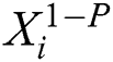to , which generates slices. The remaining useful life of each slice is computed as , which can be regarded as the total number of time steps minus the end time steps of this slice. Suppose represents the slice and is the remaining useful life. Hence, the training set is defined as , where denotes the size of the training set.

In the testing phase, we handle each unit based on its lifetime. Different from the training phase, for each unit, we use the last K time steps if its lifetime is greater than K; otherwise, we pad the lifetime to K.

Figure 2: Feature engineering (K equals 5, and the size of the padding part equals 2)

3.2 Effective Latent Representation

As shown in Part B of Fig. 3, for a given time series of the k-th training data, the auto encoder automatically extracts features and casts into a low-dimension latent space 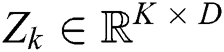, where denotes the latent space of , and D denotes the dimension of the latent space. will be used in the downstream layers. Then, is reconstructed as , where represents the time series after the reconstruction in the original space. This process can be defined as

where and denote the decoder and encoder, respectively, and can be composed of neural networks.

In order to achieve a more compact and accurate representation, the reconstructed should be as close as possible to for each . Suppose is the reconstruction loss function. The RMSE is used for the reconstruction loss function, which is given by

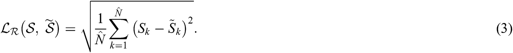
Figure 3: Structure of ACB

3.3 Temporal Convolutional Layer and Bidirectional LSTM Layer

To extract both short-term features and long-term features, convolutional layers and bidirectional LSTM layer are used, as shown in Part C of Fig. 3. Consider a given time series of k-th training data from latent space generated by the auto encoder mentioned above.

The convolutional layer slides the filters over the input time series to generate feature maps, and this can be computed by:

where refers to the convolution operator, w and b denote the 1D weight kernel and the bias, respectively, and a denotes the non-linear activation function. F is the number of feature maps, which is usually larger than D.

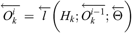
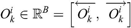
Bidirectional structures have proven to be very successful in some tasks, such as natural language processing. Accordingly, time-series data are also suitable for bidirectional models. The core idea behind Bi-LSTM lies in the fact that two separate hidden layers are utilized to process the sequence of time-series data in two directions (i.e., forward and backward) to capture the information of both the past and the future. Consider a given time series 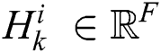of the i-th time step of the k-th training data. Two different symbols, i.e., and , are used to represent the forward and the backward processes. Eq. (5) describes the structure of Bi-LSTM:

.

Here, and are forward and backward LSTM networks, respectively. and denote the parameters of and . and are LSTM cells. B denotes the number of cells in Bi-LSTM.

Finally, a fully connected layer is used to generate the predicted RUL is given by:

where indicates the predicted RUL of the k-th training data, denotes the weight vector of the final fully connected layer, and p is the global average pooling layer.

3.4 Loss Function

In the training process, the total loss function can be divided into two parts, reconstruction loss and output loss, and is given by:

where and are the weights of the losses. The reconstruction loss has been computed in Eq. (3). To penalize the predicted RUL that is greater than the ground-truth RUL, a new P-RMSE loss is proposed and defined as follows:

where denotes the predicted RUL while denotes the ground-truth RUL. is given by:

where is the penalty term.

4  Experiments

In this section, some experiments are conducted on the publicly available C-MAPSS dataset for RUL predictions. The dataset descriptions are given in Section 4.1. Then, we employ RMSE, and the score function as metrics for performance evaluation. Next, we introduce the details of the ACB implementation. Then we use the grid search method to generate the best hyper-parameters and compare our approach with other baselines approaches. Furthermore, we evaluate the proposed model’s robustness to noise by adding random Gaussian noise.

4.1 C-MAPSS Dataset

The C-MAPSS dataset is widely used in RUL predictions as a benchmark dataset [22]. The C-MAPSS dataset is divided into four sub-datasets (from FD001 to FD004), each of which can be further divided into a training set and a testing set with different numbers of trajectories and conditions, as shown in Tab. 1. The complexity of the sub-datasets will increase with the number of operating conditions and fault conditions [23]. FD002 and FD004 are two relatively complex sub-datasets. The data are also contaminated with sensor noises.

Table 1: C-MAPSS dataset details from [16]

In each sub-dataset, data can be regarded as a 2D matrix stored in chronological order. Each row is a snapshot of information data of the current cycle. The 1st column is the engine ID, the 2nd column represents the operational cycle number, the 3rd to 5th columns list the three operating settings that have a substantial effect on the engine performance [24], and the last 21 columns present sensor values. In the training dataset, data are provided from the start to the failure point. In the testing dataset, data are provided from the start to a certain time point before the failure point.

4.2 Performance Metrics

In order to evaluate the performance, the RMSE is given by:

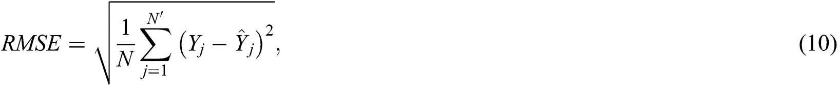
where denotes the total number of data after the augmentation, denotes the ground-truth RUL, and denotes the predicted RUL.

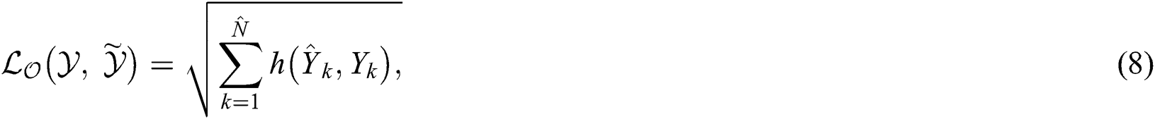
In PHM area, the score function [15] is used as follows

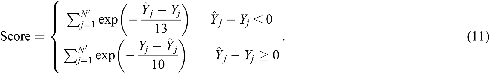
The score function was used by many studies to evaluate RUL predictions performance [25,26] and was also employed in the International Conference on Prognostics and Health Management Data Challenge. Similar to the P-RMSE loss function in Eq. (7), Eq. (11) penalizes the predicted RUL that is greater than the ground-truth RUL, and is controlled by two constants, 10 and 13.

As shown in Fig. 4, the defect of the score function is that if one predicted RUL is much larger than the ground-truth RUL, the score might be excessively large because an exponential operation is used in this function. However, the score function contains more information than the RMSE in RUL predictions.

Figure 4: Comparison of RMSE and score

4.3 Implementation Details

We implemented ACB using the deep learning library Keras. The first two layers of the encoder consist of two 1D convolution layers with a kernel size and 8-dimensional hidden states, followed by a 1D max pooling layer and a batch normalization layer. A decoder is a mirrored representation of an encoder. The softmax activation function is used in the last 1D convolution layer of the decoder. The CNN layers consist of two 1D convolution layers with 12-dimensional hidden states and a dropout layer with a 0.2 dropout rate. Meanwhile, the Bi-LSTM layer is made up of 12-dimensional hidden states and a dropout layer with a 0.2 dropout rate. A 1D max pooling layer and a batch normalization layer are also used after the CNN layers and Bi-LSTM layer. Finally, a global average pooling layer and a fully connected layer are used to generate the RUL.

4.4 Evaluation of Hyper-Parameters

Our proposed method ACB is significantly influenced by five hyper-parameters: the size of the sliding window K, the penalty term , the reconstruction loss weight , the output loss weight , and the start point of linear degradation R. We set and to 1 as default. Meanwhile, we use the grid search method to find the best values of K, , and R on the FD004 sub-dataset.

We increased from 0 to 0.8, K from 50 to 110, and R from 100 to 170. Therefore, the search space is . We traversed the entire search space to find the best set of parameters . Because the search space is too large to visualize, for better display, we kept two of the parameters unchanged and then only changed the remaining one. For example, we fixed () and then made R change from to , where n is the search range of parameter R.

In Fig. 5a, when R equals 130, the RMSE and score values are both the lowest. However, since the R value restricts the upper limit of the predicted RUL, overly large R values might induce high variance, while too small R values might lead to a high bias. We conduct the same experiments on all four sub-datasets. The conclusion is that different datasets might prefer different R values because of the different operating conditions. In a single-operations dataset like FD001 and FD003, setting R to 120 is most suitable; meanwhile, R equaling 130 is more reasonable on multi-operations datasets such as FD002 and FD004.

Note that in Fig. 5b, the curve has some fluctuations, but there is still an optimum when equals 0.3. Note that when equals 0, the P-RMSE is equivalent to the RMSE. A too-large penalty term results in over-penalization, which makes the predicted RUL less than the actual RUL. Hence, a relatively small is recommended.

Fig. 5c shows the effects of the size of the sliding window K. K indicates that how much information will be fed into models. However, excessive information or features might cause overfitting, while insufficient information might cause underfitting. K equaling 90 is suitable in our experiments.

Figure 5: Effects of the three key hyper-parameters on performance on the FD004 sub-dataset. (a) Effects on R, (b) Effects on , (c) Effects on K

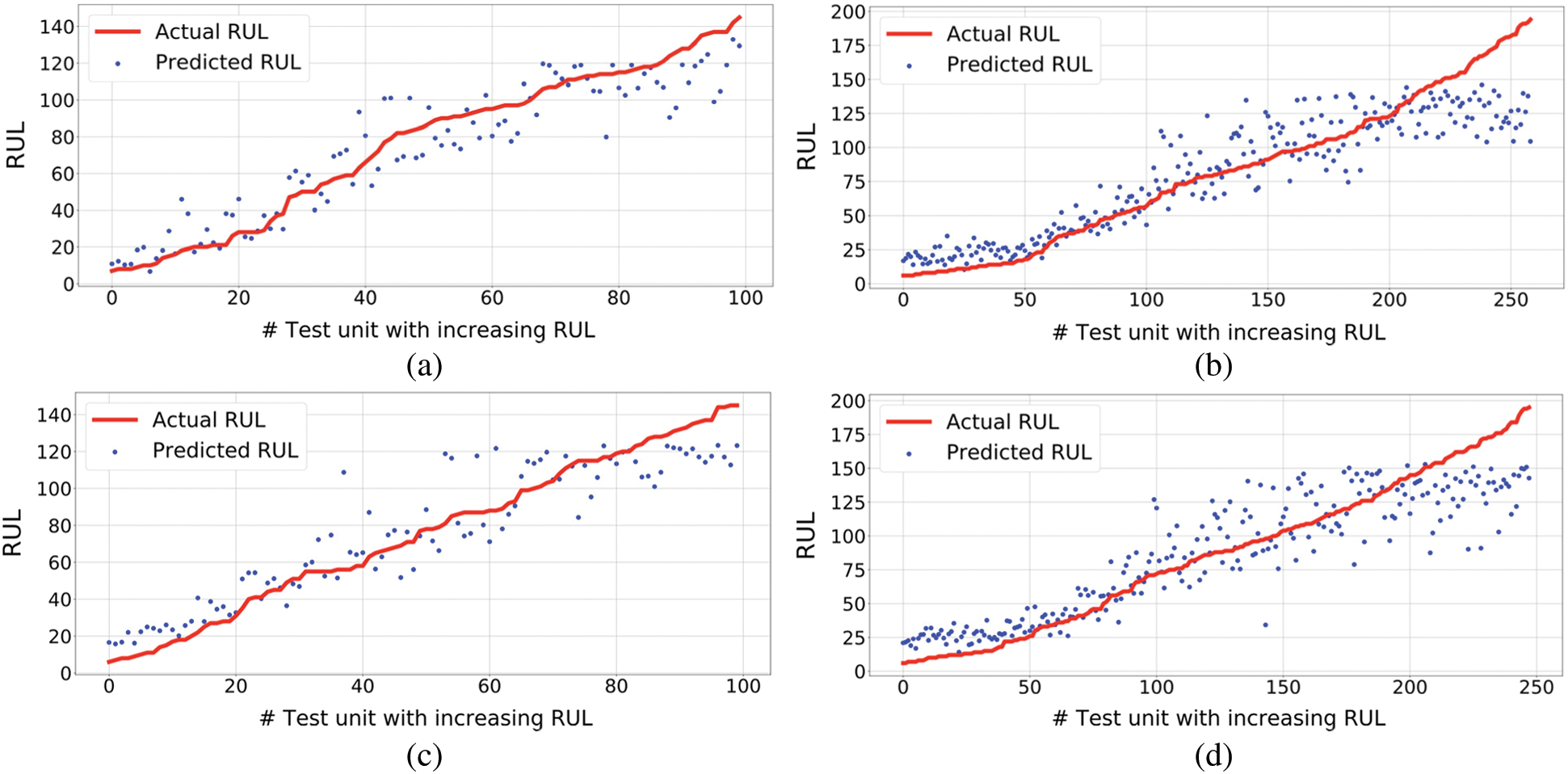
Figure 6: Result visualizations of ACB on the C-MAPSS dataset (a) FD001 visualization, (b) FD002 visualization, (c) FD003 visualization, (d) FD004 visualization

4.5 Experimental Results and Evaluation

ACB’s predicted RULs on each sub-dataset are shown in Fig. 6 with suitable hyper-parameters as mentioned in Section 4.4. In Fig. 6, test units are sorted in ascending order by the actual RUL value for the four testing datasets. Note that at the beginning of use (on the right of the figure), the degradation of a component is negligible, which results in a weaker prediction performance. Conversely, close to the left of the figure, the component is already degraded, and thus the prediction performance is significantly improved.

We also compared ACB with several state-of-the-art baselines including the CNN [17], Deep LSTM [20], Temporal Convolutional Memory Networks (Temporal CMN [10]), Light Gradient Boosting Machine (LightGBM [18]), and Convolutional Neural Network-eXtreme Gradient Boosting (CNN-XGB [19]). The Deep LSTM employs multi-layer LSTM and a multi-layer fully connected layer, which makes full use of the sensor sequence information. Temporal CMN incorporates temporal convolutions with both long-term and short-term time dependencies. Meanwhile, LightGBM uses a light gradient boosting machine to estimate the RUL, while CNN-XGB ensembles a 1*1 filter kernel and XGBoost to predict the RUL. The results are shown in Tab. 2.

Table 2: Performance comparisons with baselines (results of baselines come from their respective papers)

To better analyze these results, Fig. 7 shows a randomly selected unit from each sub-dataset. Similar to Fig. 6, the closer the component to the failure point, the more accurate the ACB’s results.

Table 3: Robustness evaluation at different noise levels on the FD004 sub-dataset

4.6 Robustness to Noise

To evaluate the robustness, we evaluated the results obtained under different noise conditions. We used the method proposed by Gugulothu et al. [13] to add noise to the FD004 sub-dataset due to its complex conditions. Each testing data in the FD004 sub-dataset, where denotes the number of time steps for the j-th component, and M denotes the number of sensors. At each time step t, was corrupted with additive Gaussian noise, which generates a new version of the testing data as follows:

As shown in Tab. 3, ACB is stable and performs well at different noise levels .

Figure 7: Results visualization of ACB on the C-MAPSS dataset. (a) Testing unit #3 in FD001, (b) Testing unit #1 in FD002, (c) Testing unit #1 in FD003, (d) Testing unit #35 in FD004

5  Conclusions

In this work, an end-to-end deep learning network combining an autoencoder, CNN, and Bi-LSTM for remaining useful life predictions was presented. The autoencoder is designed for dimensionality reduction to adapt multivariate sensor data and noisy conditions. Meanwhile, the CNN and Bi-LSTM are used for catching short-term dependencies and long-term dependencies to improve the accuracy and efficiency. Furthermore, we proposed the P-RMSE loss function to penalize the predicted RUL that is greater than the ground-truth RUL in order to avoid overestimation. ACB achieved promising results on the C-MAPSS dataset, and in some complex sub-datasets it performed better than other models. The robustness of ACB to noise was evaluated in experiments. In the future, we plan to optimize the LSTM structure and consider using some variants of the autoencoder, such as stacked denoising autoencoders and variational autoencoders, to prompt further model improvement.

Funding Statement: The authors received no specific funding for this study.

Conflicts of Interest: The authors declare that they have no conflicts of interest to report regarding the present study.

This work is licensed under a Creative Commons Attribution 4.0 International License, which permits unrestricted use, distribution, and reproduction in any medium, provided the original work is properly cited.