DOI:10.32604/csse.2021.014260
| Computer Systems Science & Engineering DOI:10.32604/csse.2021.014260 | |
| Article |
Fast Sentiment Analysis Algorithm Based on Double Model Fusion
1Sanming University, Network Center, Sanming, 365004, China
2College of Mathematics and Informatics, Fujian Normal University, Fuzhou, 350007, China
3Chengdu Institute of Computer Applications, Chinese Academy of Sciences, Chengdu, 610041, China
4University of Chinese Academy of Sciences, Beijing, 100049, China
5Sichuan Rainbow Consulting & Software Co., Ltd., Chengdu, 610041, China
*Corresponding Author: Yongxiang Gu. Email: guyongxiang19@mails.ucas.ac.cn
Received: 09 September 2020; Accepted: 02 October 2020
Abstract: Nowadays, as the number of textual data is exponentially increasing, sentiment analysis has become one of the most significant tasks in natural language processing (NLP) with increasing attention. Traditional Chinese sentiment analysis algorithms cannot make full use of the order information in context and are inefficient in sentiment inference. In this paper, we systematically reviewed the classic and representative works in sentiment analysis and proposed a simple but efficient optimization. First of all, FastText was trained to get the basic classification model, which can generate pre-trained word vectors as a by-product. Secondly, Bidirectional Long Short-Term Memory Network (Bi-LSTM) utilizes the generated word vectors for training and then merges with FastText to make comprehensive sentiment analysis. By combining FastText and Bi-LSTM, we have developed a new fast sentiment analysis, called FAST-BiLSTM, which consistently achieves a balance between performance and speed. In particular, experimental results based on the real datasets demonstrate that our algorithm can effectively judge sentiments of users’ comments, and is superior to the traditional algorithm in time efficiency, accuracy, recall and F1 criteria.
Keywords: Sentiment analysis; model fusion; Bi-LSTM; FastText
In recent years, sentiment analysis has received much more attention from both academia and industry than ever. Sentiment analysis is a common application of NLP, which uses sentiment vocabulary to determine the sentiment category. A multitude of sentiment vocabulary analysis methods have been proposed in the past decades. As an instance, according to the emotional attributes of words, Turny [1] used unsupervised learning method to calculate the Pointwise Mutual Information (PMI) to measure sentiment polarity of sentence. Kim et al. [2] classified a specific sentence as an emotional category by combining the individual sentiment of topic words, and extracted news topics from the sentence structure to predict the emotional category. In addition, Thelwall et al. [3] exploited combining grammatical and spelling rules for sentiment analysis. Since sentiment vocabulary usually changes with context information, static sentiment vocabulary is too weak for classification tasks in different context. To solve this problem, Wang et al. [4] proposed a topic-specific sentiment analysis method based on the LSTM with attention mechanism, which focused on the characteristics of different parts of the sentence through the attention mechanism, and achieved good performance on the task of sentiment classification of specific topics.
However, the features of sentiment words are largely neglected. Furthermore, Yang et al. [5] employed the attention model with sentiment symbols to strengthen the ability to capture global important information in a specific context environment, which improved the performance greatly. In addition, since the expression in Internet reviews is more flexible and new words as well as grammatical rules are created more quickly, vocabulary-based sentiment analysis methods do not adopt well in this context. On the other hand, Machine learning has been widely used in the field of short text sentiment analysis of Internet reviews, which emerges a multitude of excellent algorithms for supervised and unsupervised learning models. As an instance, Pang et al. [6] advocated the supervised learning model in sentiment classification for the first time, which performed significantly better than traditional analysis algorithms based on sentiment vocabulary. Moreover, this study also emphasized that sentiment classification is more arduous than general classification tasks. In order to improve the performance of the sentiment analysis model, researchers tried to add different features to the supervised model [7–10]. The diversity of different features improves the performance of the model, but the supervised model requires a lot of labeled data, which is commonly costly, resulting in a high labor cost in real world applications. On the contrary, unlabeled data is easy to obtain, which is more flexible and applicable in real world applications. Towards this end, researchers used semi-supervised learning methods or unsupervised methods in sentiment classification to reduce dependence on labeled data, such as labeling propagation, co-training, and active learning. As an instance, with the benefit of collaborative training, Wan [11] focused on cross-language sentiment classification and trained a Chinese sentiment classification model using annotated English data sets. Cheng et al. [12] incorporated explicit sentiment signals in textual terms and implicit sentiment signals, compiling the sentiment signal from a single social network into a coherent model for unsupervised sentiment analysis.
A multitude of researchers used supervised learning to exploit contextual knowledge regularization for sentiment analysis. Wu et al. [13] considered the co-occurrence of words and used the PMI index to calculate the similarity of words. Tai et al. [14] proposed extracting various contextual sentiment knowledge from unlabeled samples and expressing it as the relationship between sentiment expressions. They proposed three constraints: Grammatical constraints, co-occurrence constraints and vocabulary constraints. In addition, Wu et al. [15] introduced a method using graph-based supervised learning to calculate word similarity.
Inspired by recent advance of deep neural networks, Vaswani et al. [16] introduced Transformer, which is a deep neural network based solely on attention mechanism, and has achieved impressive results on a variety of NLP tasks. Furthermore, many variants of the Transformer model have emerged in recent years. The representative works include Bidirectional Encoder Representations from Transformers (BERT) [17], XLNet [18] and ERNIE [19]. Among them, BERT is a milestone model, which is an attention-based Transformer model and auto-encoding model. BERT was trained on a large-scale unlabeled data to obtain a general word vector representation, which results demonstrated that this learning strategy can achieve state-of-the-art in tasks such as text classification and translation. Based on this work, Manish et al. [20] implemented fine-grained sentiment classification based on BERT. However, an ocean of parameters in BERT and BERT-like models place restrictions on practical applications.
Most of the current researches tend to exploit the sentiment relationship between vocabulary, and do not make full use of the semantic relationship in context. Moreover, when convert the text into a word vector, a time-consuming word vector algorithm is required, which has poor time efficiency. Towards this end, we introduce a new fast sentiment classification method called FAST-BiLSTM. First of all, FastText [21] was trained to get the basic classification model, which can generate pre-trained word vectors as a by-product. Secondly, Bi-LSTM utilizes the generated word vectors for training and then merges with FastText to make comprehensive sentiment analysis. The fusion model can further exploit the semantic information in the context and achieve higher time efficiency than traditional models.
FastText is a supervised word vector algorithm, its model structure is consistent with the Continuous Bag-of-Words (CBOW) model. The CBOW model structure is shown in Fig. 1.

Figure 1: CBOW model structure
There are two main differences between FastText and CBOW model. First of all, the input data and prediction target are different. CBOW inputs the sum or average of the vectors which have removed the target word. While FastText turns bag-of-words into bag-of-features to use more order information. That is, the input xi in Fig. 2 is no longer just a word, but can also add bigram or trigram information. Secondly, the prediction target in CBOW is a word in the context. While in FastText, prediction target is the category of the current input text. To get the text category, FastText provides a framework for text representation and text classification. The essence is to predict an index given an index collection.
The FastText model structure is shown in Fig. 2. The entire model is divided into three layers: input layer, hidden layer and output layer. The input layer inputs words represented by multiple vectors, the output layer outputs a specific target, and the vector of the hidden layer is the superimposed average value of multiple word vectors.

Figure 2: FastText model structure
The objective function of FastText is as shown below:

where N is the number of samples; yn is the corresponding category of the n-th sample; f represents the softmax loss function; xn is the normalized feature of the n-th sample; A is the weight parameter of the Embedding layer; B is the weight parameter of hidden layer.
The traditional word vector tools like word2vec treat each word as an atom, ignoring the morphological features inside the word. Such as “apple” and “apples”, the pair words have a host of shared characters, that is, they have similar internal morphology. In traditional word2vec models, the internal morphological information of words is lost because they are converted into different ids. FastText solved this problem by utilizing character-level n-grams to represent a word. For the word “apple”, assuming the value of n is 3, its trigrams have “<ap”, “app”, “ppl”, “ple”, “le>“, where < means suffix, > means prefix. Therefore, these trigrams can be used to represent the word “apple”. Furthermore, the superimposed vector of these 5 trigrams can be used to represent the word vector of “apple”. This is better for word vectors generated by low-frequency words. Because their n-grams can be shared with other words.
2.2 Bidirectional Long Short-Term Memory Network
In our FAST-BiLSTM model, Bi-LSTM network is used as one of the fusion models. The unidirectional LSTM infers the later part from the previous information, but sometimes only focusing at the previous words cannot make full use of the global information. The bidirectional LSTM network is designed for this case, it is a kind of time series Recurrent Neural Network (RNN), which is specially designed to solve the long-term dependence problem of general RNN. The key to solve the problem of gradient dissipation is that LSTM introduces the cell state in the time series and the structure of the “gate” between cells. State refers to the carrier of information circulation in the neural network, which allows the information in the data to be conveyed to the next cell. LSTM has three types of gate structures: Forget gate, input gate and output gate [22]. The LSTM network structure is shown in Fig. 3.

Figure 3: LSTM network structure
In order to demonstrate the operation mechanism of LSTM vividly and concisely, the definition of symbols concerned with Eqs. (2)–(7) is given firstly. Wf, Wi, Wc are the weighted matrices and bf, bi, bc are biases of LSTM to be learned during training. xt stands for the inputs of LSTM cell unit at time t and ht-1 is the vector of hidden layer at time t-1.  and
and  are used to represent the sigmoid function and element-wise multiplication, respectively.
Forget gate is in charge of making decisions on retaining or discarding information. This process needs to take advantage of the property that the output of the sigmoid function is between 0 and 1. The specific process is that the current cell passes the input of the current state and the hidden information of the previous cell to the sigmoid function. The closer the output value of sigmoid function is to 0, the more likely it should be discarded. The information transmission in forget gate can be expressed by Eq. (2).

Input gate is in charge of updating the cell state. This process also requires the property of the sigmoid function, but the input is the hidden information of the previous layer and the current input information. The output value determines which information needs to be updated. Analogously, the closer the output value is to 1, the more crucial it is and the more it needs to be updated. The information transmission in input gate can be expressed by Eq. (3).

Output gate is in charge of determining the next hidden state which refers to the previous input information. What the sigmoid function receives at this moment is the previous hidden state information and the current input information. The new cell state information will be passed to the tanh function at this time. The current hidden state is obtained by multiplying the output of the tanh function and the output of the sigmoid function. The information of the current hidden state will be passed to the next cell in the same way. The calculation formulas for the LSTM unit can be expressed as follows:


Although LSTM solved the long-term dependency problem, it cannot use the later information of the text. Bi-LSTM considers the global information in context. Its implementation principle is: the word vectors generated by the embedding layer are used as the input of two LSTM networks with opposite timing. The forward LSTM can obtain the forward information of the input sequence, and the backward LSTM can obtain the backward information. The following information of the sequence is then calculated by vector splicing to obtain the final hidden layer representation. In this way, the hidden layer of each word in the text sequence contains complete context information.
3 Double Model Fusion Algorithm
The fast text sentiment analysis algorithm based on double-model fusion is shown in Fig. 4. Right part is the FastText model that accepts clean text data, which consists of a hierarchical softmax and a linear network with n-gram features. Specifically, the label is encoded with Huffman coding, which greatly reduces the number of targets predicted by the model. Apart from generating a FastText classification model, this part will also get pre-trained word vector embeddings. Left part is the Bi-LSTM classification model. This part uses the pre-trained word vectors provided by the FastText model for word embedding, and then do semantic mining. When the last LSTM unit outputs, the information is sent to the fully connected layer and softmax layer for classification. After obtaining two classification models, these models are stacked and merged to further improve the performance. Based on the above description, the overall algorithm flows of fast text sentiment analysis are as follows:
1. Data cleaning, invalid or empty data will be removed in this step.
2. Word segmentation tool is used to segment the text. Here, we use the Harbin Institute of Technology’s LTP word segmentation tool.
3. Input the data into the FastText model to train the binary classification model and generate word vectors at the same time.
4. Load the word vector in Step 3 and use the Bi-LSTM model to train a binary classification model.
5. Combine the FastText model in Step 3 with the Bi-LSTM model in Step 4 for stacking model fusion.

Figure 4: Model diagram of fast text sentiment analysis algorithm based on double model fusion
For machine learning and deep learning, the performance of a single model is often worse than the model fusion. In proposed algorithm, the stacking model fusion is used to combine the Bi-LSTM and FastText. The training and prediction processes are shown in Fig. 5.

Figure 5: Two model fusion process
The whole processes of model fusion are as follows:
1. Vector representations of text training data are divided into five parts.
2. Use the Bi-LSTM model and the FastText model to train four of all parts, then predict the training set that are not used for training and test set. Next, change the selected training sets for training and the setting used for verification, and repeat Step 2 until the prediction results of complete training sets are obtained.
3. For the five combinations, perform Step 2 respectively to obtain five models and the corresponding cross-validation prediction results, namely P1, P2, P3, P4 and P5.
4. Use five models to predict the corresponding testing set respectively, and the prediction results of the testing set are obtained as T1, T2, T3, T4 and T5.
5. Take P1~5 and T1~5 as the training sets and testing sets of the next layer.
4 Experimental Design and Analysis
The two datasets used in the experiment are all crawled from real Internet e-commerce data, one is from the online hotel reservation reviews, and the other is from takeaway platform reviews. The description of the datasets is shown in Tab. 1.

When evaluating the results of the classification, we use three common evaluation indicators, they are accuracy, recall and F1 score. Firstly, the following definitions are given: True Positive (TP), which is a positive sample predicted by the model as positive; False Positive (FP), which is a negative sample predicted by the model to be positive; False Negative (FN), which is the positive sample that is predicted to be negative by the model; True Negative (TN), which is the negative sample that is predicted to be negative by the model. Then, accuracy, recall and F1 score can be calculated as follows:


In this experiment, five commonly used classification algorithms are selected for comparison with FAST-BiLSTM. These five classification algorithms are described in detail as follows:
1. Bayes, an algorithm that uses knowledge of probability and statistics for classification, uses Bayes’ theorem to predict the probability of a sample belongs to each category, and selects the most likely category as the final result.
2. Random Forest (RF), uses multiple related decision trees to randomly build a forest classifier. While a new sample is inputted, it will be classified by every decision tree, to determine which category the sample belongs to, and then classifies it to the category which selected the most.
3. K-Nearest Neighbors (KNN), according to the unlabeled data, compares each feature of the new data with the corresponding feature of the data in the sample set, and then the algorithm extracts the closest data classification label in the sample set. Select the first K most similar data in the sample dataset, and choose the category that appears most among the K most similar data as the category of the new data [23].
4. LSTM, a type of temporal neural network, the model will not only pay attention to the current time information all the time, but also pay attention to what information can be used for the current time in the previous processing, and does classification according to the text semantic information.
5. CNN-LSTM, uses the LSTM network to extract the key semantic information of the sentence, distinguishes the text according to the extracted semantics; then uses CNN to extract the features of the text and does classification. This experiment combines them, first extracts the key semantics of the text, and then extracts the key features of the semantics to classify the text.
To verify the effectiveness of our algorithm, experiments were carried out on the Windows platform with following environment: Intel(R)-Core (TM) i7-8750U 2.20 GHz CPU, GTX 1660 GPU and 24 GB memory. Then, keras framework was used to build the FastText and Bi-LSTM model. The main hyperparameters of the model are shown in Tab. 2.
Table 2: Important hyperparameter setting in experiment

In the tuning process of FAST-BiLSTM algorithm, the parameters of the model were adjusted. Among them, there are four main parameters that are vital to the model: minCount, dimension of word vector, number of iterations in FastText and number of neurons in Bi-LSTM. After carefully adjusting, the influences of these hyperparameters are shown in Figs. 6–9.
The influence of minCount in FastText is shown in Fig. 6. The minCount represents the threshold of minimum word frequency, which menas that word with frequency less than the threshold will be removed directly. When the corpus is relatively large, the threshold should be small, because the low frequency will be arduous to fit. We set the value of minCount to (2,3,4,5,6,7,8) for testing. Finally, the model has the highest accuracy, recall and F1 score at the value of 5. This is because when the minCount value is 5, the most reasonable selection of word frequency is ensured. When the value is too small, the low-frequency words cannot be filtered out, which reduces the fitting ability of the model. While the value is too big, useful words in the text will be deleted, which will make the performance worse.
The influence of dimension of word vector in FastText word vector is shown in Fig. 7. We set the value of word vector dimension to (16, 32, 64, 128) for experiments. When the value is 64, the model has the highest accuracy, recall and F1 score. From our own perspective, this may because when the word vector dimension is set to 64, it perfectly matches the size of the text data volume. If the value is too small, the information in the corpus will not be expressed, and the model effect will be worse due to insufficient model fitting. While the value is too big, the word vector will become a sparse matrix, which increases the arduousness of training, the performance will also get worse.
The influence of number of iterations in FastText model is shown in Fig. 8. All data pass through the neural network once and return once. This process is called an epoch. The choice of epoch should be considered in conjunction with the learning rate. In this paper, the learning rate is set to 0.05, and the Adam optimizer is chosen as optimizer. The times of iterations are respectively selected as (20, 30, 40, 50, 60, 70, 80, 90) for experiments. When the number of iterations is set to 70, the model has the highest accuracy, recall and F1 score, which demonstrates the model reaches the optimal state when the number is 70. This is because that too few iterations will result in underfitting, while too many iterations will result in overfitting, either of these two cases will make performance worse.
Fig. 9 demonstrates the influence of number of neurons in the Bi-LSTM model. When the number of neurons is set to 100, the model is optimal. From the change in the evaluation value in Fig. 9, it can be inferred that while the number of neurons in the LSTM network is too small, the model has a weak ability to extract features. While the number of neurons is large, model’s fitting ability is strong, but too many neurons will result in a surge of the model parameters. As a consequence, not only the risk of overfitting will increase but also the training time will prolong. Finally, we set the number of Bi-LSTM neurons to 100, which is the most appropriate.

Figure 6: The influence of mincount value in FastText

Figure 7: The influence of dimension of word vector in FastText

Figure 8: The influence of number of iterations in FastText

Figure 9: The influence of number of neurons in Bi-LSTM
In order to make a better comparison between FAST-BiLSTM and other algorithms, 5-fold cross-validation method is used to test and evaluate. For data partition, the data are randomly shuffled and selected for experiment. Tab. 3 demonstrates the comparison results of FAST-BiLSTM and other five algorithms in accuracy, recall and F1 score using dataset 1. For fair comparison, word2vec method is adopted for comparison algorithm to get default word vectors. According to the results given in Tab. 3, it can be seen that the accuracy of the proposed algorithm is 7.1%, 6.1%, 8.7%, 3.8%, 2.5% higher than that of Naive Bayes, Random Forest, K-nearest, LSTM and CNN-LSTM, respectively. The recall rate increased by 4.1%, 3.7%, 5.5%, 2.0%, 1.8%; in terms of F1 evaluation criteria, our algorithm still has great advantages, and the F1 increased by 3.4%, 3.2%, 4.9%, 2.7%, 2.2%, respectively. On dataset 2, FAST-BiLSTM also manifests similar advantages. Tab. 4 demonstrates the experimental comparison results of FAST-BiLSTM and other five different algorithms using dataset 2. The accuracy increased by 5.5%, 4.5%, 6.2%, 3.1%, 2.3%; the recall increased by 7.2%, 4.8%, 8.2%, 3.7%, 2.5%; and the F1 increased by 4.7%, 4.3 %, 6.1%, 3.7%, 2.9%. From the analysis, it can be seen that the performance of FAST-BiLSTM is better on dataset 2 too. The same performance of the double sets of data proves the effectiveness of FAST-BiLSTM. Moreover, our algorithm has more obvious advantages in terms of time efficiency. Fig. 10 demonstrates the comparison of the time consumption of FAST-BiLSTM with other algorithms on the datasets. It is not arduous to see through observation that FAST-BiLSTM has a significant improvement in time efficiency compared with other algorithms. Concretely, compared with the other five algorithms (Naive Bayes, Random Forest, K Neighbor, LSTM, CNN-LSTM), the improvements of time efficiency on dataset 1 are 38%, 46%, 31%, 55%, 61%, respectively; on the dataset 2 are 49%, 56%, 43%, 57%, 64%, respectively. The huge improvement on time efficiency is invaluable for application because shortening the model training time can reduce the consumption of machine resources, save the cost of scientific personnel for training models, speed up the iteration of the model, and thus multiply the development efficiency.
Table 3: Experiments conducted on dataset 1

Table 4: Experiments conducted on dataset 2

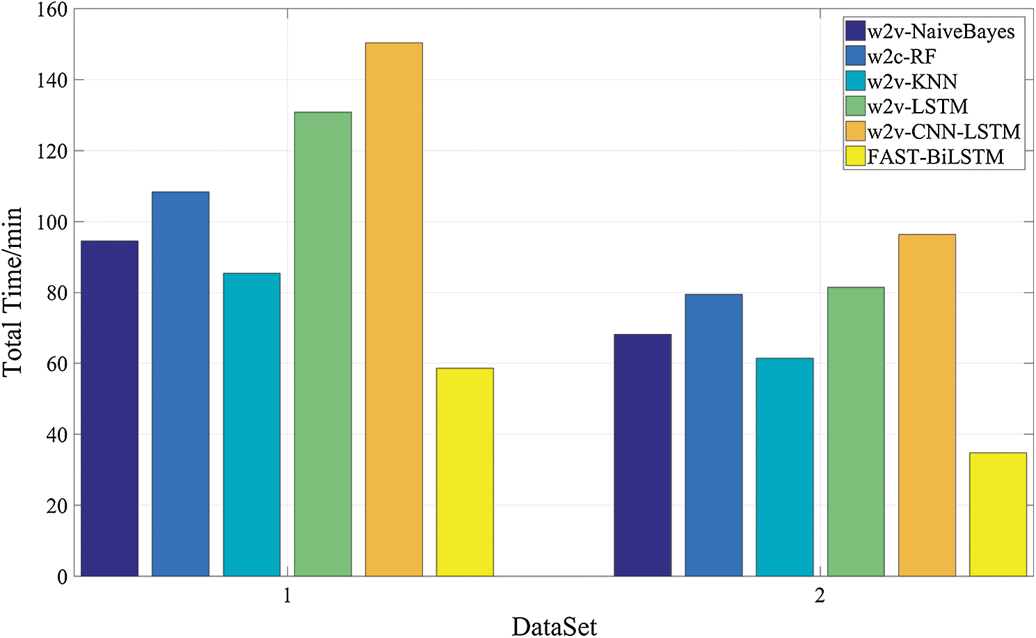
Figure 10: Comparison of total time spent by different algorithms
In this paper, we proposed a fast sentiment analysis algorithm, called FAST-BiLSTM, to solve the problems on sentiment analysis. Our algorithm is carried out by fusing the FastText and Bi-LSTM models. First of all, FastText has a fast speed for linear fitting and can generate pre-trained word vectors as a by-product. Secondly, Bi-LSTM uses the generated word vectors for training and then merges with FastText to make comprehensive sentiment analysis. Compared with the traditional word2vec methods, it has an obvious advantage in time efficiency. In order to demonstrate the performance of FAST-BiLSTM, we compare our algorithm with five commonly used algorithms on two datasets in different fields. The results manifest that the time efficiency of the algorithm is improved more than 30%, and FAST-BiLSTM can sufficiently extract contextual semantic information from texts, it is superior to other algorithms in accuracy, recall and F1 score. Moreover, our experimental results indicate that FAST-BiLSTM has achieved considerable performance in text sentiment analysis tasks at a low computational cost, and it is invaluable for practical application.
Despite the overall performance of FAST-BiLSTM is good and the time efficiency is improved especially, the classification performance can further be improved greatly. The subsequent research will focus on how to improve the classification performance. On the other hand, it will also focus on applying the algorithm to a wider range of fields, such as students’ sentiment analysis, online public opinion analysis, etc.
Funding Statement: This work is supported by the National Science Foundation of China (No. 61771140), the 2017 Natural Science Foundation of Fujian Provincial Science & Technology Department (No. 2018J01560) and the 2016 Fujian Education and Scientific Research Project for Young and Middle-aged Teachers (JAT170522).
Conflicts of Interest: The authors declare that they have no conflicts of interest to report regarding the present study.
1. P. D. Turney. (2002). “Thumbs up or thumbs down? Semantic orientation applied to unsupervised classification of reviews,” in Proc. 40th Annual Meeting on Association for Computational Linguistics, Stroudsburg, PA, USA, pp. 417–424. [Google Scholar]
2. S. M. Kim and E. Hovy. (2004). “Determining the sentiment of opinions,” in Proc. 20th Int. Conf. on Computational Linguistics, Geneva, CH, pp. 1367–1373. [Google Scholar]
3. T. Mike, B. Kevan, P. Georgios, C. Di and K. Arvid. (2010). “Sentiment in short strength detection informal text,” Journal of the American Society for Information Science & Technology, vol. 61, no. 12, pp. 2544–2558. [Google Scholar]
4. Y. Wang, M. Huang, X. Zhu and L. Zhao. (2016). “Attention-based LSTM for aspect-level sentiment classification,” in Proc. Conf. on Empirical Methods in Natural Language Processing, Austin, Texas, USA, pp. 606–615. [Google Scholar]
5. Z. Y. Sen, Z. Jia, H. G. Juan and J. Y. Ru. (2018). “Microblog sentiment analysis method based on a double attention model,” Journal of Tsinghua University, vol. 58, no. 2, pp. 122–130. [Google Scholar]
6. B. Pang, L. Lee and S. Vaithyanathan. (2018). “Thumbs up? Sentiment classification using machine learning techniques,” in Proc. Conf. on Empirical Methods in Natural Language Processing, Brussels, Belgium, pp. 79–86. [Google Scholar]
7. F. Koto and M. Adriani. (2015). “HBE: Hashtag-based emotion lexicons for twitter sentiment analysis,” in Proc. 7th Forum for Information Retrieval Evaluation, New York, NY, USA, pp. 31–34. [Google Scholar]
8. A. Giachanou and F. Crestani. (2016). “Like it or not: A survey of twitter sentiment analysis methods,” ACM Computing Surveys, vol. 49, no. 2, pp. 1–41.
9. X. C. Huang, Y. H. Rao, H. R. Xie, T. L. Wong and F. L. Wang. (2017). “Cross-domain sentiment classification via topic-related TrAdaBoost,” in Proc. Association for the Advancement of Artificial Intelligence Conf., San Francisco, USA, pp. 4939–4940.
10. A. B. Goldberg and X. Zhu. (2006). “Seeing stars when there aren’t many stars: Graph-based semi-supervised learning for sentiment categorization,” in Proc. TextGraphs: The 1st Workshop on Graph Based Methods for Natural Language Processing, New York, NY, USA, pp. 45–52. [Google Scholar]
11. X. Wan, “Co-training for cross-lingual sentiment classification,” in Proc. 47th Annual Meeting of the ACL and the 4th IJCNLP of the AFNLP, Suntec, Singapore, pp. 235–243, 2009, [Google Scholar]
12. K. Cheng, J. Li, J. Tang and H. Liu. (2017). “Unsupervised sentiment analysis with signed social networks,” in Proc. 31st AAAI Conf. on Artificial Intelligence, San Francisco, California, USA, pp. 3429–3435. [Google Scholar]
13. F. Wu, Y. Song and Y. Huang. (2015). “Microblog sentiment classification with contextual knowledge regularization,” in Proc. Twenty-Ninth AAAI Conf. on Artificial Intelligence, Palo Alto, California, USA, pp. 2332–2338. [Google Scholar]
14. Y. J. Tai and H. Y. Kao. (2013). “Automatic domain-specific sentiment lexicon generation with label propagation,” in Proc. Int. Conf. on Information Integration and Web-Based Applications & Services, New York, NY, USA, pp. 53–62. [Google Scholar]
15. F. Z. Wu, S. X. Wu, Y. F. Huang, S. F. Huang and Y. Qin. (2016). “Sentiment domain adaptation with multi-level contextual sentiment knowledge,” in Proc. 25th ACM Int. on Conf. on Information and Knowledge Management, New York, NY, USA, pp. 949–958. [Google Scholar]
16. A. Vaswani, N. Shazeer, N. Parmar, J. Uszkoreit, L. Jones et al. (2017). , “Attention is all you need,” in Proc. Advances in Neural Information Processing Systems, Long Beach, California, USA, pp. 6000–6010. [Google Scholar]
17. J. Devlin, M. W. Chang, K. Lee and K. Toutanova. (2019). “BERT: Pre-training of deep bidirectional transformers for language understanding,” in Proc. Conf. of the North American Chapter of the Association for Computational Linguistics, Minneapolis, Minnesota, USA, pp. 4171–4186. [Google Scholar]
18. Z. Yang, Z. Dai, Y. Yang, J. Carbonell, R. R. Salakhutdinov et al. (2019). , “XLNet: Generalized autoregressive pretraining for language understanding,” in Proc. Advances in Neural Information Processing Systems, New York, NY, USA, pp. 5754–5764. [Google Scholar]
19. Z. Zhang, X. Han, Z. Liu, X. Jiang, M. Sun et al. (2019). , “ERNIE: Enhanced language representation with informative entities,” in Proc. Annual Meeting of the Association for Computational Linguistics, Florence, Italy, pp. 1441–1451. [Google Scholar]
20. M. Munikar, S. Shakya and A. Shrestha. (2019). “Fine-grained sentiment classification using BERT,” in Proc. Artificial Intelligence for Transforming Business and Society (AITBKathmandu, Nepal, pp. 1–5. [Google Scholar]
21. A. Joulin, E. Grave, P. Bojanowski and T. Mikolov. (2017). “Bag of tricks for efficient text classification,” in Proc. 15th Conf. of the European Chapter of the Association for Computational Linguistics, Valencia, Spain, pp. 427–431. [Google Scholar]
22. S. X. Jian, C. Z. Rong, W. Hao, Y. D. Yan, W. W. Kin et al. (2015). , “Convolutional LSTM network: A machine learning approach for precipitation nowcasting,” in Proc. Advances in Neural Information Processing Systems, Montreal, Canada, pp. 802–810. [Google Scholar]
23. J. M. Ding, G. Q. Liu and H. Li. (2015). “The application of improved random forest in the telecom customer churn prediction,” Pattern Recognition and Artificial Intelligence, vol. 28, no. 11, pp. 1041–1049. [Google Scholar]
 | This work is licensed under a Creative Commons Attribution 4.0 International License, which permits unrestricted use, distribution, and reproduction in any medium, provided the original work is properly cited. |