DOI:10.32604/csse.2021.014342
| Computer Systems Science & Engineering DOI:10.32604/csse.2021.014342 | |
| Article |
Bivariate Beta–Inverse Weibull Distribution: Theory and Applications
Department of Statistics, Faculty of Science, King Abdulaziz University, Jeddah, Saudi Arabia
*Corresponding Author: Muhammad Qaiser Shahbaz. Email: mkmohamad@kau.edu.sa
Received: 15 September 2020; Accepted: 11 November 2020
Abstract: Probability distributions have been in use for modeling of random phenomenon in various areas of life. Generalization of probability distributions has been the area of interest of several authors in the recent years. Several situations arise where joint modeling of two random phenomenon is required. In such cases the bivariate distributions are needed. Development of the bivariate distributions necessitates certain conditions, in a field where few work has been performed. This paper deals with a bivariate beta-inverse Weibull distribution. The marginal and conditional distributions from the proposed distribution have been obtained. Expansions for the joint and conditional density functions for the proposed distribution have been obtained. The properties, including product, marginal and conditional moments, joint moment generating function and joint hazard rate function of the proposed bivariate distribution have been studied. Numerical study for the dependence function has been implemented to see the effect of various parameters on the dependence of variables. Estimation of the parameters of the proposed bivariate distribution has been done by using the maximum likelihood method of estimation. Simulation and real data application of the distribution are presented.
Keywords: Bivariate beta distribution; inverse Weibull distribution; conditional moments; maximum likelihood estimation
The probability distributions are widely used in many areas of life. Standard probability distributions have been extended by various authors to increase the applicability of a given baseline distribution. The exponentiated distributions, proposed by Gupta et al. [1], extend a baseline distribution by exponentiation. The beta generated distributions, proposed by Eugene et al. [2], generalize a baseline distribution by using logit of the beta distribution. The cumulative distribution function (cdf) of the Beta-G distributions is

where  is the cdf of any baseline distribution and
  is the complete beta function defined as

The density function of any member of the Beta–G family of distributions is written as

Another method of generating new distributions has been proposed by Cordeiro et al. [3] by using the cdf of Kumaraswamy distribution, proposed by Kumaraswamy et al. [4]. The proposed family is referred to as the Kumaraswamy–G (Kum–G) family of distributions and its cdf is

A general method of generating new distributions has been proposed by Alzaatreh et al. [5] by using the cdf of any distribution and this method is known as the T-X family of distributions. The cdf of new distribution by using the T-X family of distributions is

where  is the density of any random variable defined on
  , where d1 can be –∞ and d2 can be +∞, and
  is any function of
  such that
  and
and  .
.
The Beta–G, the Kum–G and the T-X family of distributions provide basis to obtain a new univariate distribution by using the cdf,  , of any baseline distribution. Different authors have proposed several new distributions by using these families, for example beta-normal by Eugene et al. [2], beta-Weibull by Famoye et al. [6], beta-inverse Weibull by Hanook et al. [7], Kum-inverse Weibull by Shahbaz et al. [8], gamma-normal by Alzaatreh et al. [9], exponentiated-gamma distribution by Nadarajah et al. [10], among others.
Several situations arise where we are interested in the simultaneous modeling of two random variables, for example we may be interested in the simultaneous study of arrival and departure time of the customers at a service station. In such situations some suitable bivariate distribution is required. The bivariate beta distribution, proposed by Olkin et al. [11], is a useful bivariate distribution to model random variables which represent proportion of some events of interest. The density function of the bivariate beta distribution is

where  is extended beta function defined as

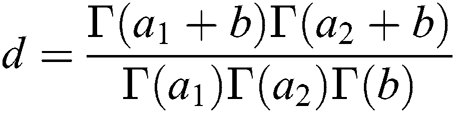
and  is the complete gamma function defined as
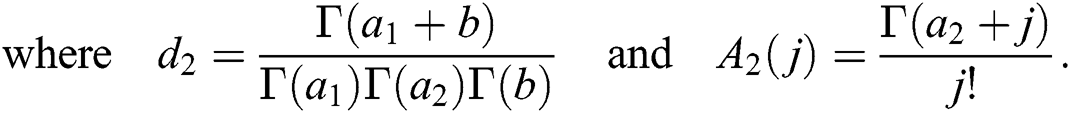
The bivariate beta distribution has been used by Sarabia et al. [12] to propose the bivariate Beta-G1G2 (BB-G1G2) family of distributions. The joint cdf of the proposed family is
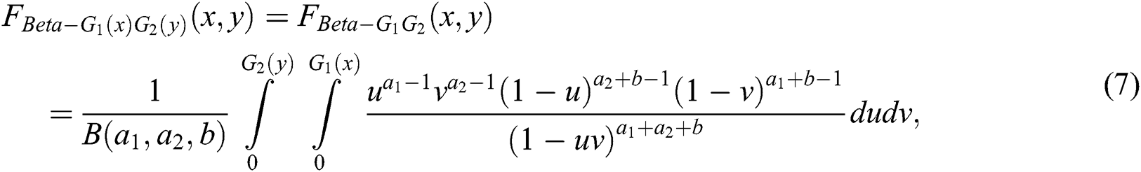
for  . The density function of the BB-G1G2 family of distributions is
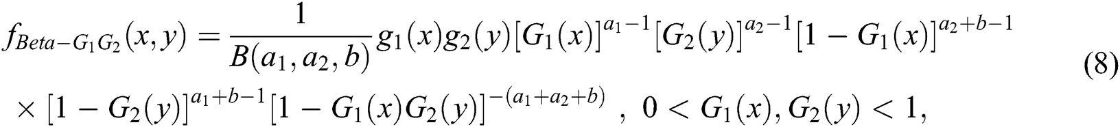
and  . It is also shown by Sarabia et al. [12] that the density (8) can be written as

where  is the density function of the beta-G distribution, given in (2).
The BB-G1G2 family of distributions has not be explored and in this paper we will propose a new bivariate beta-inverse Weibull distribution. The structure of the paper is given below.
A new bivariate beta-inverse Weibull distribution is proposed in Section 2 alongside its marginal and conditional distributions. Some properties of the proposed distribution are obtained in Section 3. Estimation of the parameters of the proposed bivariate distribution is given in Section 4. Section 5 contains simulation and real data applications. Conclusions and recommendations are given in Section 6.
2 The Bivariate Beta-Inverse Weibull Distribution
The inverse Weibull distribution, also known as the Fréchet [13] distribution, is a useful lifetime distribution. The density and distribution functions of the inverse Weibull distribution are

and

where  is the rate and
  is the shape parameter. A random variable X having the inverse Weibull distribution is written as
  . Now, suppose that the random variable X has
  and the random variable Y has
  distribution with cdf’s

Using the distribution functions of X and Y in (7), the distribution function of the bivariate beta-inverse Weibull (BBIW for short) distribution is
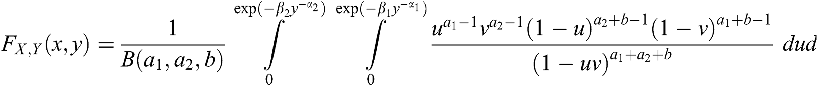
or

where

is the extended incomplete beta function and

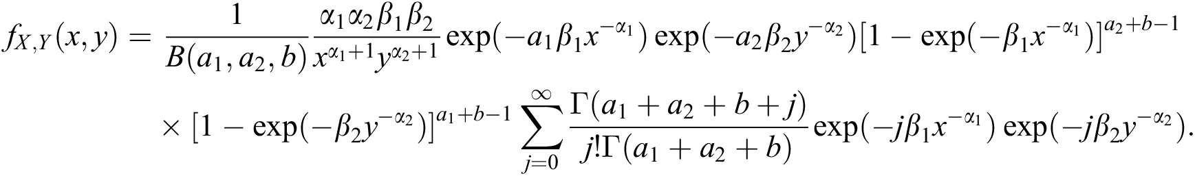
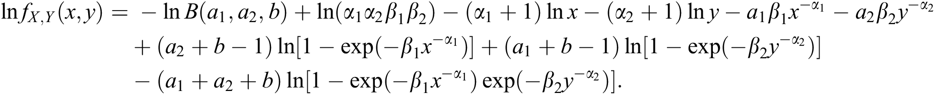
is the extended incomplete beta function ratio. The density function of the BBIW distribution is written from (8) as

and  . The random variables X and Y having joint density (15) is written as
  . The plots of the density function for
  and for different choices of the other parameters are shown in Fig. 1 below.
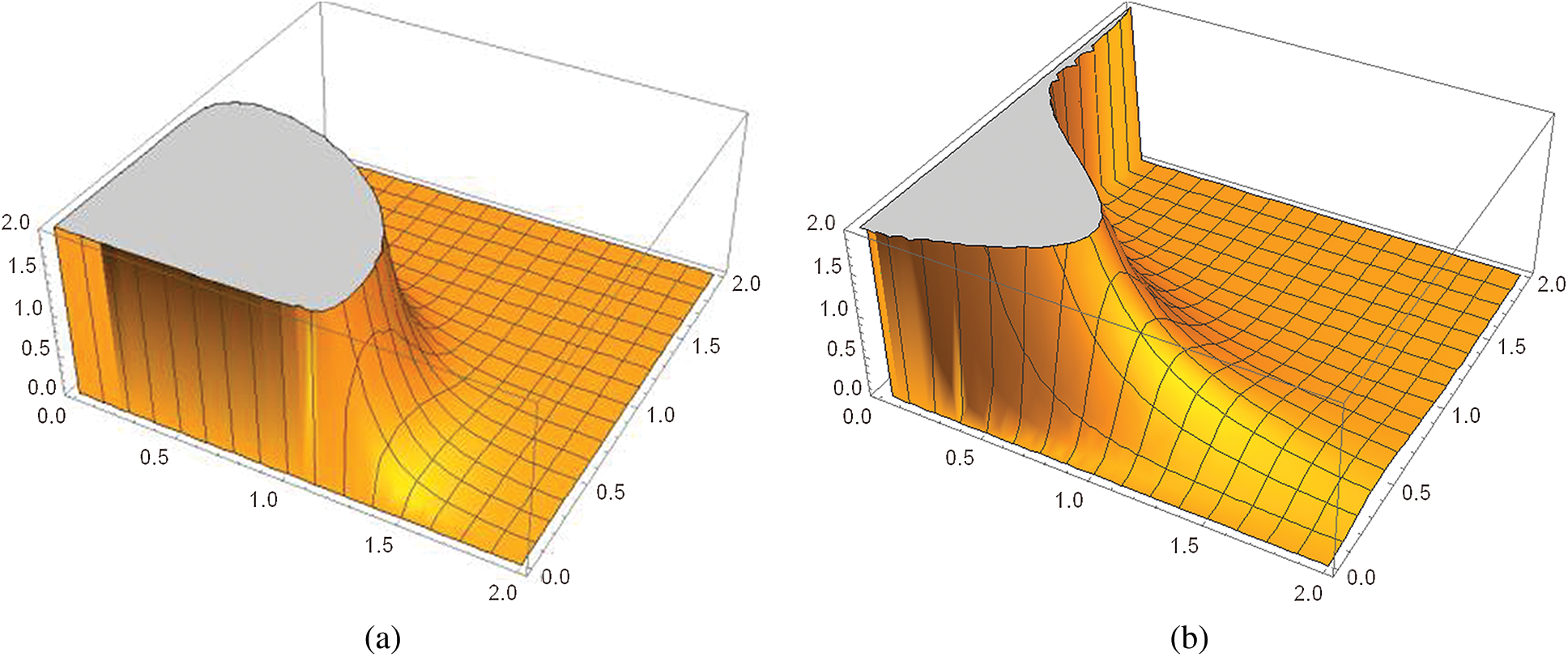
Figure 1: Plot of density function of bivariate beta inverse Weibull distributions for various choices of parameters. (a)  (b)
(b) 
The plot of joint distribution function for  ,
,  ,
,  ,
,  ,
,  and
and  is given in Fig. 2.

Figure 2: The distribution function of bivariate beta-inverse Weibull distribution
The BBIW distribution provides various other distributions as special case. For example, for  we have the bivariate beta inverse exponential (BBIE) distribution and for
  the distribution reduces to the bivariate beta inverse Rayleigh (BBIR) distribution.
The joint hazard rate function of the distribution is obtained by using
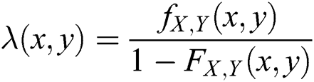
and is given as
The hazard rate function can be computed for different values of the parameters.
The density function of the BBIW distribution can also be written in the form of beta-inverse Weibull density functions as

where  is the density function of the beta-inverse Weibull random variable with parameter vector
  .
.
The marginal distributions of X and Y are obtained, from (15), below.
Now
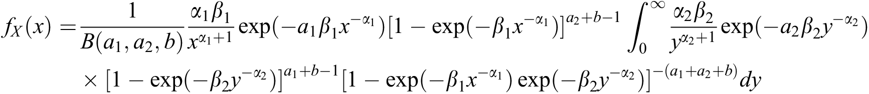
Making the transformation  , we have

or

which is density function of  . Similarly, it can be shown that the marginal distribution of Y is
  .
.
The conditional distribution of Y given X is readily obtained from (15) and (17) and is

Similarly, the conditional distribution of X given Y is

The conditional distributions are useful in computing conditional moments.
In the following we will obtain some useful expansions for the joint density function of BBIW distribution. For this, we will use following expansions, for any real a,

Now, the density function of the BBIW distribution is

Using following series expansion

we have
Re-arranging, the above density can be written as
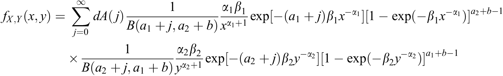
or

where  is the density function of beta-inverse Weibull distribution. Also
and
From (20), it is easy to see that the joint density function of the BBIW distribution is the weighted sum of product of marginal density functions of the beta-inverse Weibull distributions.
The expansion of the density function, given in (20), can also be written as the weighted sum of density functions of the inverse Weibull distributions. For this, we use following expansions

and

Using these expansions in (20), the density function of the BBIW distribution is written as
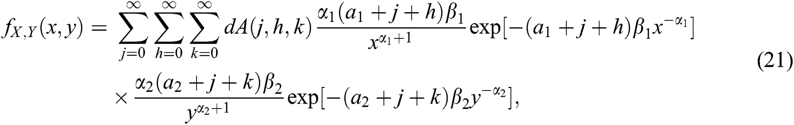
or

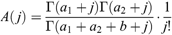
where  is the density function of the inverse Weibull random variable with parameters
  and
and

From (21), we can see that the density function of the BBIW distribution is the weighted sum of product of the inverse Weibull density functions. The expression (21) is useful in computing moments of the distribution.
The expansion for the conditional density function of X given Y is readily obtained by using

in (19) and is
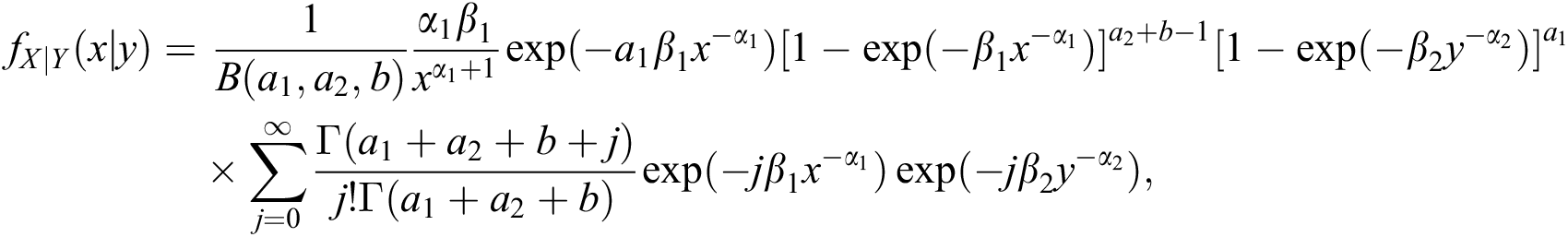
or
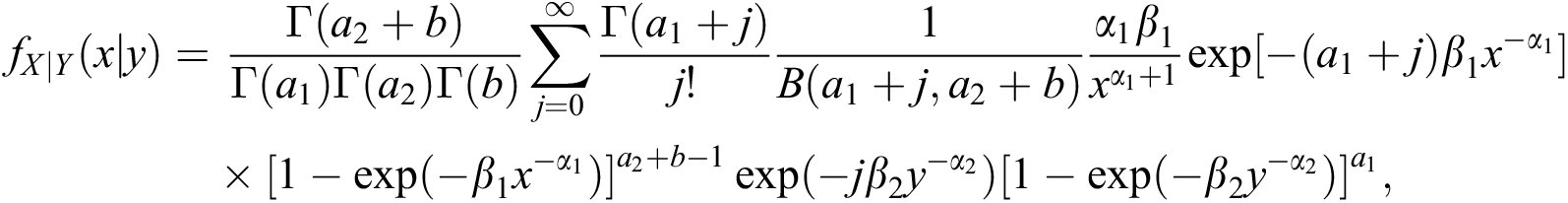
or


The expansion of the conditional density function of Y given X is similarly written as

The expansions (22) and (23) are helpful in computing the conditional moments of the distribution.
3 Properties of the Distribution
In this section some properties of the BBIW distribution are discussed. These properties include joint, marginal and conditional moments and are discussed in the following sub-sections.
3.1 Product and Ratio Moments of the Distribution
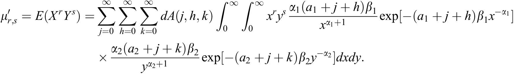
The product and ratio moments of the BBIW distribution are obtained by using the joint density function, given in (15), or the expansion of the density function, given in (21). It is easier to obtain the product and ratio moments from (21) and are obtained below.
The (r,s)th product moment for two random variables is defined as
Using the joint density function of the BBIW distribution, the expression for the product moment is
Making the transformations  and
and  , the expression for the product moment for the BBIW distribution is

which exists for  and
and  .
.
The (r,s)th ratio moment for two random variables is defined as
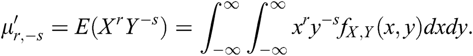
Using the joint density function of the BBIW distribution, the ratio moment is
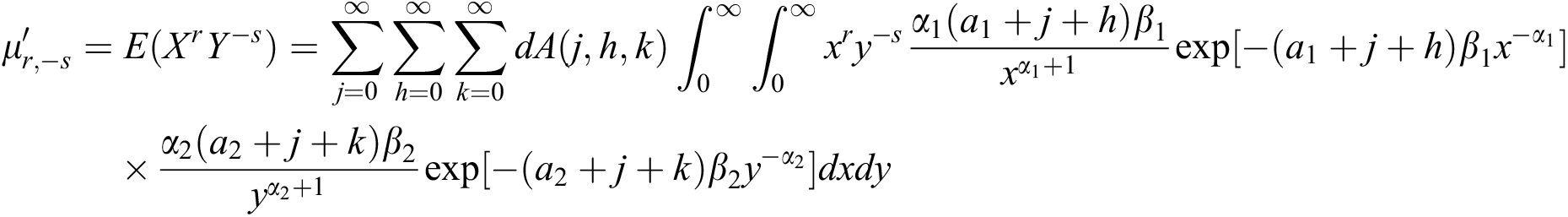
Again making the transformations  and
and  , the expression of the ratio moment for the BBIW distribution is

Similarly, the expression for the ratio moment,  , for the BBIW distribution is

It is to be noted that the parameters a1, a2 and b has no effect on the means and variances of the random variables X and Y as these are controlled by parameters  and
and  .
.
3.2 Conditional Moments of the Distribution
The conditional moment of a distribution is useful in studying the behavior of one variable under the conditions on the other variable. In case of a bivariate distribution we can compute conditional moment of X given Y = y and of Y given X = x. In the following, the conditional moments for the BBIW distribution are obtained.
The conditional moment of X given Y = y is computed as
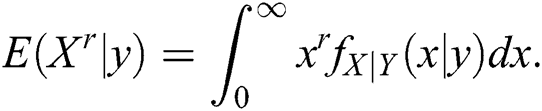
Now, using the conditional distribution of X given Y = y, from (22), we have

Using the density function of the beta-inverse Weibull distribution, we have
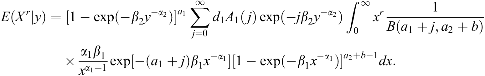
Now, using the expansion

in above equation we have
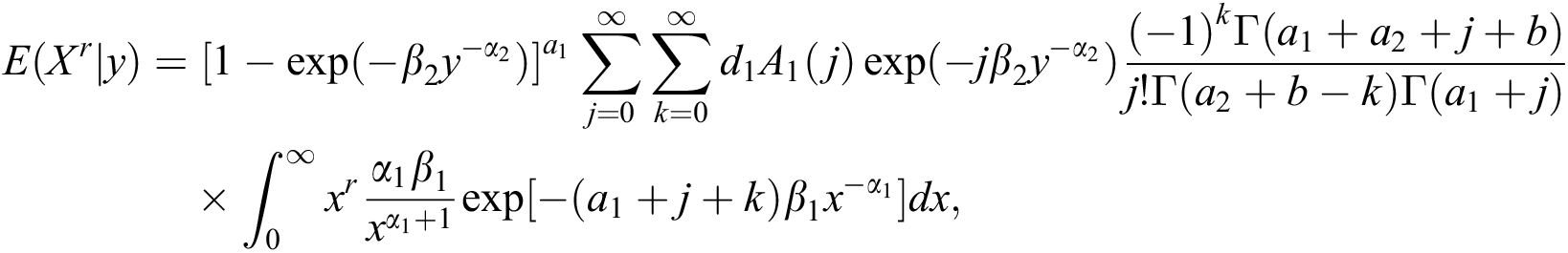
or

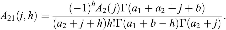
where

Similarly, the expression for the conditional moment of Y given X = x is

where
The conditional means and variances can be obtained from (27) and (28).
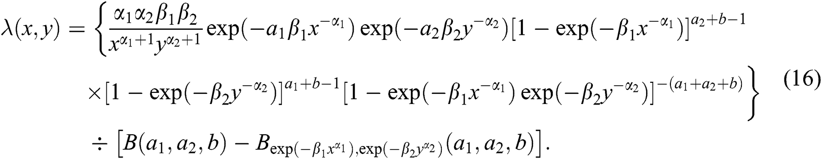
3.3 The Dependence Function and Correlation Coefficient
The dependence function for a bivariate distribution is, given by Holland et al. [14],
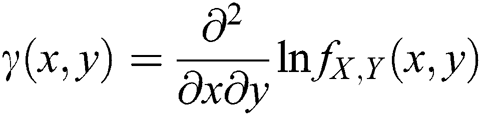
and Sarabia et al. [12] has shown that the dependence function for the BB–G1G2 family is

Using the density and distribution functions of the inverse Weibull distribution in (29), the dependence function for the BBIW distribution is

which is always positive. It is to be noted that the dependence function is different from the linear correlation coefficient which is to be computed from the product moment. The values of correlation coefficient for different combinations of the parameters are given in Tab. 1 below. The values of correlation coefficient indicate that the effect of a1 and a2 on the correlation coefficient is positive, that is increase in the values of a1 and a2 will increase the linear correlation between X and Y for the BBIW distribution. The effect of other parameters on the correlation coefficient is negative, that is increase in b,  and
and  will decrease the correlation coefficient.
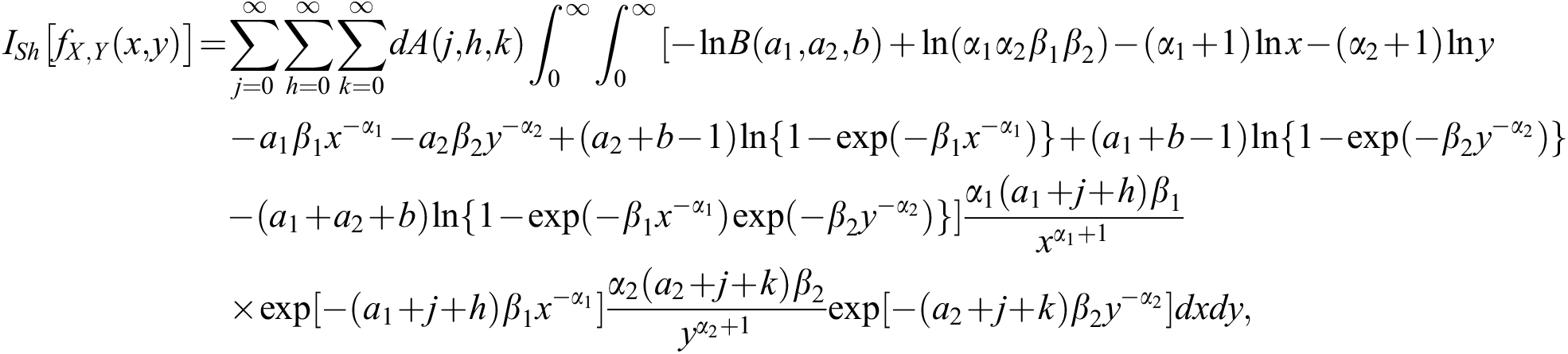
The Shannon entropy, Shannon [15], in a bivariate distribution is defined as

Now, for the BBIW distribution we have
Using this in above equation, the Shannon entropy for the BBIW distribution is
Table 1: Correlation coefficient between X and Y for the BBIW distribution

or
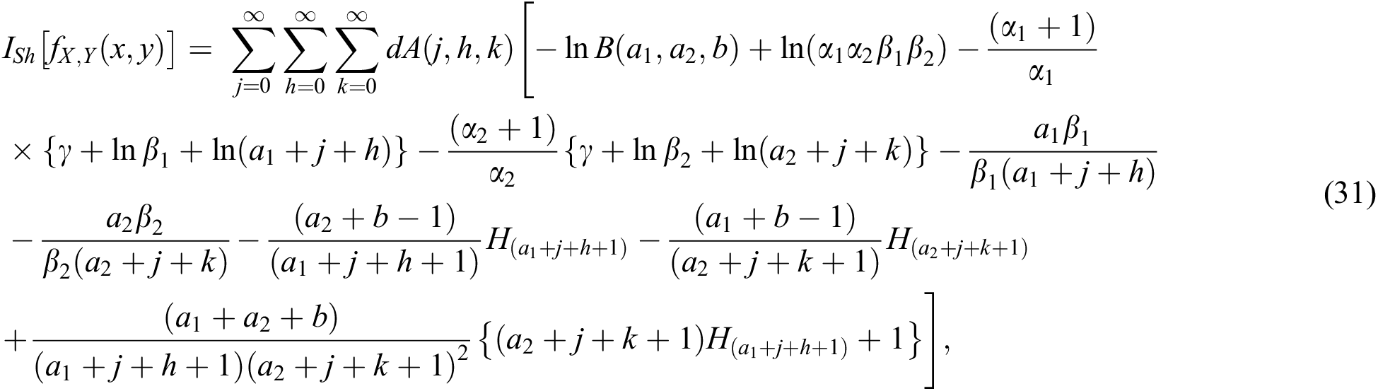
where  is the Euler’s gamma and
  is the harmonic number of order k.
The random sample from the BBIW distribution can be generated by using the conditional distribution method. In this method the random sample from a bivariate distribution is generated using following two steps
• Generate a random variate from the marginal distribution of X.
• Generate a random variate from the conditional distribution of Y given X = x.
Using this method, the random sample from the BBIW distribution can be generated by using following algorithm
• Generate a random variate X from the beta-inverse Weibull distribution with given parameters 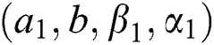 and denote it by x.
• Generate a random variate Y from the conditional distribution of Y given X = x, given in (18).
• The pair (x,y) is a single random observation from the BBIW distribution.
• Repeat the process until sample of size n is obtained.
The random variates from the beta-inverse Weibull distribution can be easily obtained by using any of the R package; for example Newdistns, by Nadarajah et al. [16] or MPS by Teimouri [17].
In this section, parameter estimation of the BBIW distribution is presented. For this, we first see that the likelihood function for a sample of size n from the distribution is
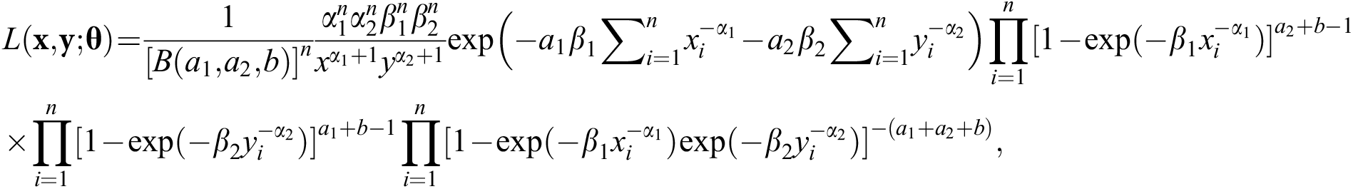
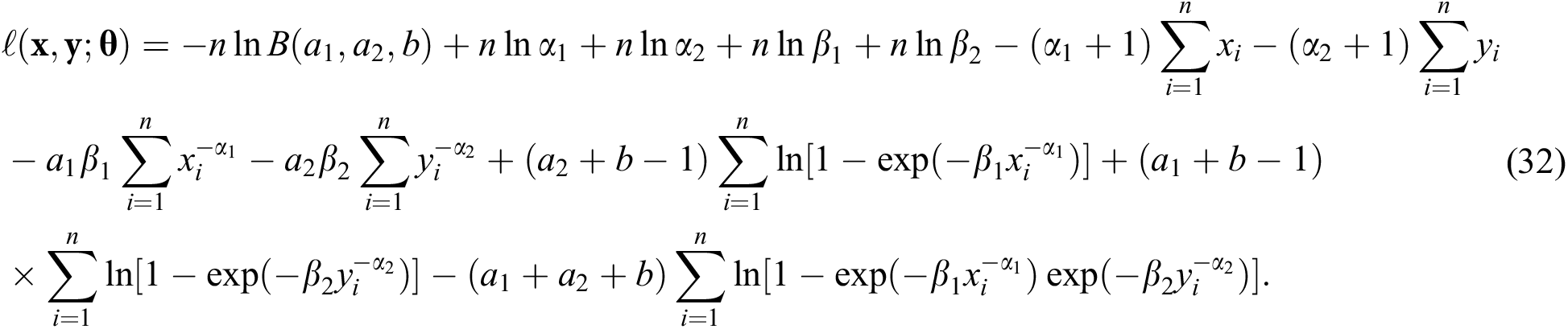
where  . The log-likelihood function is
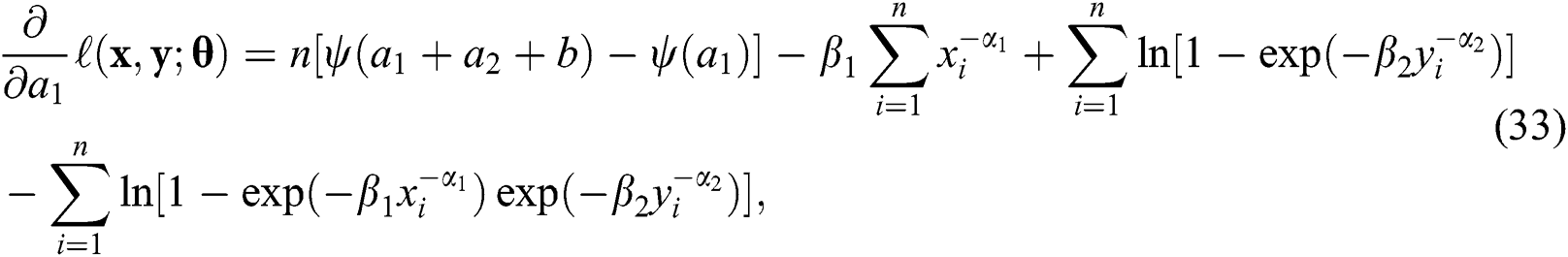
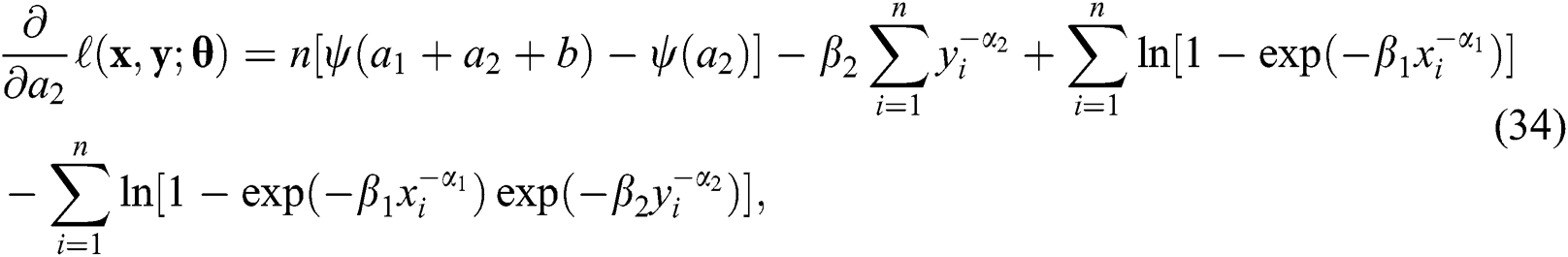
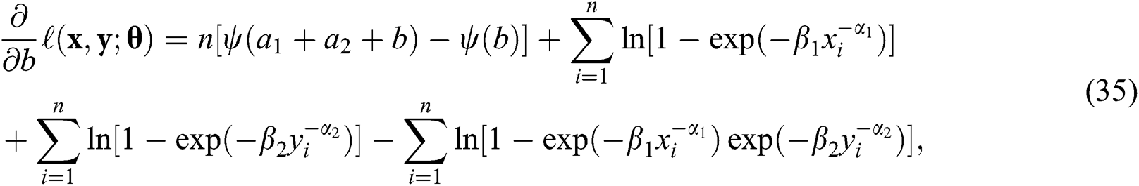
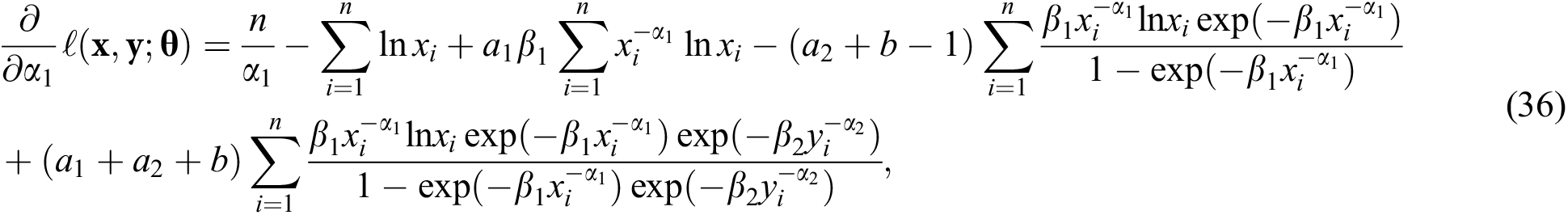
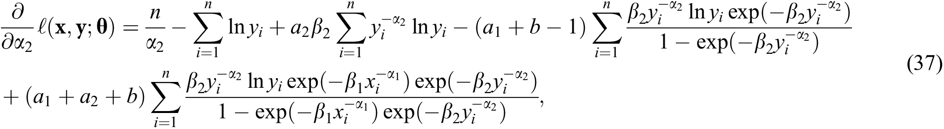
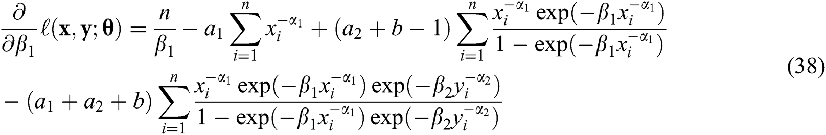
The derivatives of the log-likelihood function with respect to the unknown parameters are
and
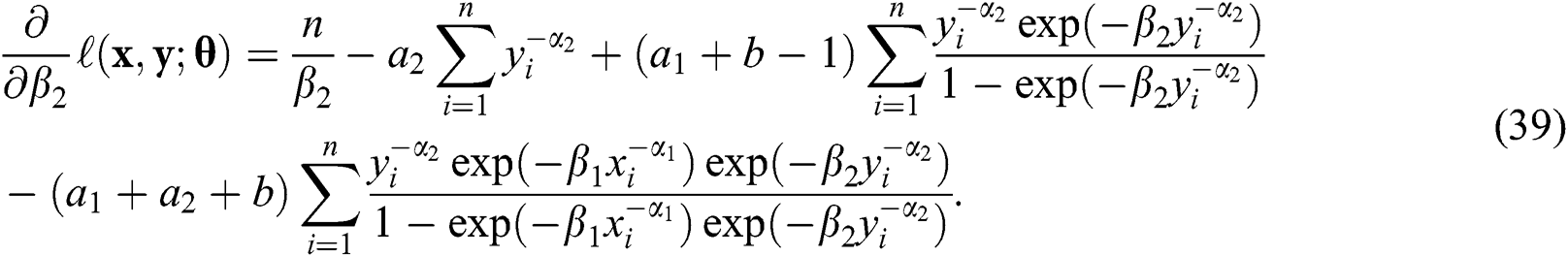
The maximum likelihood estimates are obtained by equating the derivatives, given in Eqs. (33) and (39), to zero and simultaneously solving the resulting equations.
In this section some numerical applications of the proposed BBIW distribution are given. We will first give a simulation study to see the performance of the maximum likelihood estimates and then we will apply the proposed BBIW distribution on a real data set. These applications are discussed in the following subsections.
In the following, simulation results for the proposed BBIW distribution are given. The algorithm for the simulation study is given below:
1. Draw random sample of a specific size from the BBIW distribution, for specific values of the parameters, using the procedure given in Section 3.4.
2. Obtain maximum likelihood estimates of the parameters for the generated sample.
3. Repeat Steps 1 and 2 for the specific number of simulations.
4. Obtain average value of the estimates and the standard errors.
In our simulation study, random samples of sizes 50, 100, 200 and 500 are drawn and the results are simulated for 50000 times. The results of simulation study are given in Tab. 2 below (standard error of the estimate is in the parenthesis).
The simulation results indicate that the estimate converges to the true parameter value with increase in the sample size. We can also see that the standard error of the estimate decreases with increase in the sample size.
Table 2: Simulation results for the BBIW distribution

In this section, a real data application of the proposed BBIW distribution is given. We have used data on GNI per capita of all the countries of the world for 2016 (as X) and for 2017 (as Y). The data is obtained from UNDP site http://hdr.undp.org/en/data [18]. For the analysis, the data is transformed by dividing actual values with 10000. The bivariate histogram of the data is shown in Fig. 3 below.

Figure 3: Bivariate histogram of the GNI data
We have fitted three bivariate distributions to the data including the bivariate beta inverse Weibull (BBIW) distribution, the bivariate Weibull (BW) distribution, proposed by Shahbaz et al. [19], and the bivariate inverse Weibull (BIW) distribution obtained by using F-G-M family with density.

Results of the fitted models are given in Tab. 3 below.
Table 3: Results of fitted distributions to GNI data

From the table, we can see that the BBIW distribution is the best fit to the data as it has smallest AIC. The fitted BBIW distribution is shown in Fig. 4 below.

Figure 4: Fitted BBIW distribution for GNI data
The graph of the fitted BBIW distribution is reasonably close to the bivariate histogram of the data.
In this paper a new bivariate beta inverse Weibull distribution is proposed by using the logit of bivariate beta distribution. The distribution is very flexible and is useful in modeling of the complex data. The properties of the distribution have been studied and it is found that the correlation coefficient is controlled by combination of three parameters  ,
,  and b. The proposed bivariate beta inverse Weibull distribution has been fitted to the world GNI data of two years and it is found that the proposed BBIW is better fit as compared with the other models involved in the study
Funding Statement: This project was funded by the Deanship of Scientific Research (DSR), King Abdulaziz University, Jeddah under grant number (D-153-130-1441). The author, therefore, gratefully acknowledge the DSR technical and financial support.
Conflicts of Interest: The authors declare no conflict of interest regarding the publication of this paper.
1. R. D. Gupta and D. Kundu. (2001). “Exponentiated exponential family: An alternative to gamma and Weibull,” Biometrical Journal, vol. 43, pp. 117–130. [Google Scholar]
2. N. Eugene, C. Lee and F. Famoye. (2002). “Beta-normal distribution and its applications,” Communications in Statistics: Theory & Methods, vol. 31, no. 4, pp. 497–512. [Google Scholar]
3. G. M. Cordeiro and M. de Castro. (2011). “A new family of generalized distributions,” Journal of Statistical Computations and Simulations, vol. 81, no. 7, pp. 883–898. [Google Scholar]
4. P. Kumaraswamy. (1980). “A generalized probability density function for double bounded random processes,” Journal of Hydrology, vol. 46, no. 1–2, pp. 79–88. [Google Scholar]
5. A. Alzaatreh, C. Lee and F. Famoye. (2013). “A new method of generating families of continuous distributions,” Metron, vol. 71, no. 1, pp. 63–79. [Google Scholar]
6. F. Famoye, C. Lee and O. Olumolade. (2005). “The beta-Weibull distribution,” Journal of Statistical Theory and Applications, vol. 4, pp. 121–136. [Google Scholar]
7. S. Hanook, M. Q. Shahbaz, M. Mohsin and B. M. G. Kibria. (2013). “A note on beta-inverse Weibull distribution,” Communications in Statistics: Theory & Methods, vol. 42, no. 2, pp. 320–335. [Google Scholar]
8. M. Q. Shahbaz, S. Shahbaz and N. S. Butt. (2012). “The Kumaraswamy inverse Weibull distribution,” Pakistan Journal of Statistics and Operation Research, vol. 8, no. 3, pp. 479–489. [Google Scholar]
9. A. Alzaatreh, F. Famoye and C. Lee. (2014). “The gamma-normal distribution: Properties and applications,” Computational Statistics and Data Analysis, vol. 69, pp. 67–80. [Google Scholar]
10. S. Nadarajah and A. K. Gupta. (2007). “The exponentiated gamma distribution with application to drought data,” Calcutta Statistical Association Bulletin, vol. 59, no. 1–2, pp. 29–54. [Google Scholar]
11. I. Olkin and R. Liu. (2003). “A bivariate beta distribution,” Statistics and Probability Letter, vol. 62, no. 4, pp. 407–412. [Google Scholar]
12. J. M. Sarabia, F. Prieto and V. Jorda. (2014). “Bivariate beta-generated distributions with applications to well-being data,” Journal of Statistical Distributions & Applications, vol. 1, pp. 15. [Google Scholar]
13. M. Fréchet. (1927). “Sur la loi de probabilité de l'écart maximum,” Annales de la societe Polonaise de Mathematique, vol. 6, pp. 93. [Google Scholar]
14. P. W. Holland and Y. J. Wang. (1987). “Dependence function for continuous bivariate densities,” Communications in Statistics: Theory & Methods, vol. 16, no. 3, pp. 863–876. [Google Scholar]
15. C. Shannon. (1948). “A mathematical theory of communication,” Bell System Technical Journal, vol. 27, no. 3, pp. 379–423. [Google Scholar]
16. S. Nadarajah and R. Rocha. (2016). “Newdistns: An R package for new families of distributions,” Journal of Statistical Software, vol. 69, pp. 1–32. [Google Scholar]
17. M. Teimouri, “MPS: An R package for modeling new families of distributions. arXive:1809.02959v1, 2018. [Google Scholar]
18. United Nations Development Programme. 2019. [Online]. Available: http://hdr.undp.org/en/data. [Google Scholar]
19. S. H. Shahbaz, M. Al-Sobhi, M. Q. Shahbaz and B. Al-Zahrani. (2018). “A new multivariate Weibull distribution,” Pakistan Journal of Statistics and Operation Research, vol. 14, no. 1, pp. 75–88. [Google Scholar]
 | This work is licensed under a Creative Commons Attribution 4.0 International License, which permits unrestricted use, distribution, and reproduction in any medium, provided the original work is properly cited. |