DOI:10.32604/csse.2021.014343
| Computer Systems Science & Engineering DOI:10.32604/csse.2021.014343 | |
| Article |
Highway Cost Prediction Based on LSSVM Optimized by Intial Parameters
1School of Mechanics and Civil Engineering, China University of Mining and Technology-Beijing, Beijing, 100083, China
2School of Information Engineering, Yangzhou University, Yangzhou, 225127, China
*Corresponding Author: Shuang Liu. Email: liushuang_0122@163.com
Received: 15 September 2020; Accepted: 19 October 2020
Abstract: The cost of highway is affected by many factors. Its composition and calculation are complicated and have great ambiguity. Calculating the cost of highway according to the traditional highway engineering estimation method is a completely tedious task. Constructing a highway cost prediction model can forecast the value promptly and improve the accuracy of highway engineering cost. This work sorts out and collects 60 sets of measured data of highway engineering; establishes an expressway cost index system based on 10 factors, including main route mileage, roadbed width, roadbed earthwork, and number of bridges; and processes the data through principal component analysis (PCA) and hierarchical cluster analysis. Particle swarm optimization (PSO) is used to obtain the optimal parameter combination of the regularization parameter  and the kernel function width coefficient
  in least squares support vector machine (LSSVM). Results show that the average relative and mean square errors of the PCA-PSO-LSSVM model are 0.79% and 10.01%, respectively. Compared with BP neural networks and unoptimized LSSVM model, the PCA-PSO-LSSVM model has smaller relative errors, better generalization ability, and higher prediction accuracy, thereby providing a new method for highway cost prediction in complex environments.
Keywords: Highway; least squares support vector machine (LSSVM); particle swarm optimization (PSO); principal component analysis (PCA); hierarchical cluster analysis
According to traditional highway engineering estimation method, calculating its cost is an extremely perplexed task. With the rapid development of mathematical modeling methods and computer technology, experts at home and abroad have studied various mathematical models or computer simulation means for project cost forecasting. Regression analysis methods were commonly used [1] in the early foreign literature and were later combined with other probability analysis model [2]. In recent years, artificial neural network-based cost prediction approaches have become prevalent. Domestic scholars have applied methods, such as fuzzy mathematics [3], grey system theory [4], genetic algorithm [5], system dynamics [6], and big data [7], for the cost prediction of engineering projects.
A large number of documents apply BP neural network [8] for cost prediction. Owing to the slow convergence speed, these documents are liable to fall into a local minimum. Support vector machine (SVM) has excellent learning ability and can be used for small sample size, thereby avoiding structure selection, and the local minima of the neural network. SVM has elicited extensive attention for in-depth study. SVM has several problems. First, its algorithm setting parameters are based on empirical values. Second, its implementation is complicated and difficult. Lastly, it has slow training speed. The least squares support vector machine (LSSVM), as an improved SVM algorithm, inherits a series of excellent features, such as the SVM kernel function, the principle of structural risk minimization, and small sample size. Complex quadratic programming problem is transformed into a simpler linear equation solving problem, which shortens training time and improves solution speed greatly [9].
Particle swarm optimization (PSO) algorithm uses real numbers to find the optimal parameters. The algorithm has strong versatility, fast convergence, and is easier to leap to local optimal information. It has been widely used in parameter optimization. Consequently, the PSO algorithm is used to determine the optimal parameters of LSSVM and improve calculation accuracy [10].
Through preliminary research on the aforementioned algorithms, this work sorts out and collects the data of existing highways, establishes a sample set, processes the samples through hierarchical cluster analysis and principal component analysis (PCA), builds a PCA-PSO-LSSVM [11] highway engineering prediction model, and compares the proposed model with the BP neural network and the unoptimized LSSVM model.
2 Basic Principle of PCA-PSO-LSSVM
PCA is an index dimensionality reduction method based on mathematical ideas. It uses the orthogonal transformation in linear programming to reduce the given variables with correlation to a small number of uncorrelated comprehensive variables. These new comprehensive variables carry most of the important information of the original indicators, and the relationship of complex matrix is simplified to achieve the dimensionality reduction of indicators [12]. The specific steps are presented as follows:
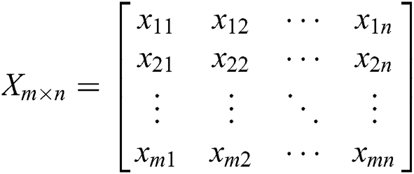
Step 1: Select the initial sample. Assuming that population  has n samples
  , and each sample has m-dimensional variables. Thus, the matrix of the observation data is denoted as:
Step 2: Standardize the original data. The formula is expressed as follows:

where
 : j\x97 is a random variable;
 : mean of the jth variable;
 : standard deviation of the jth variable.
Step 3: Calculate the correlation coefficient matrix of  and use
  to find the eigenvalue
  and its eigenvector
  .
.  .
.
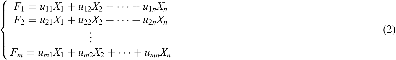
Step 4: Obtain M  principal components by calculation:

Step 5: Calculate the principal component contribution rate and cumulative contribution rate. Compute the contribution rate of the principal component according to
  . The cumulative contribution rate of the first
  principal component is
  . When the cumulative contribution rate of the current
  principal component reaches over 85%, the first q principal component is used as a new indicator.
Kennedy and Eberhart proposed PSO in 1995. This algorithm has the advantages of simplicity, easy implementation, no gradient information, and few parameters. It is particularly suitable for real number optimization problems. It also has a profound intelligent background that is suitable for scientific research, particularly for engineering applications [13]. The main principles are presented as follows:
 particles are found in the D-dimensional space; Particle
  position:
 ); Particle
  velocity:
  ; and the best position in history that particle
  has experienced:
  .
.


where
 : inertia weight factor;
 : learning factors, usually a value of 2;
 : [0,1] random function of value;
 : number of iterations.
The main principle of the mathematical model of the LSSVM regression algorithm is presented as follows. The training sample set  , where
  is the
  d-dimensional input vector, and
  is the predicted value of the corresponding input, is given. Subsequently, the regression function is:

where
 : weight vector;
 : offset.
Different from SVM, LSSVM selects the square of the error  as the loss function in the optimization objective while changing the constraints into equality constraints. When using the principle of structural risk minimization, the optimization problem becomes:
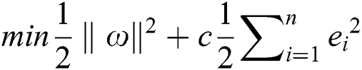

where
 : regularization parameters;
 : error vector.
The Lagrangian function is established to solve the above-mentioned problem:

The optimal solution satisfies the KKT optimization condition, and the partial derivatives of 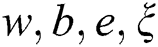 in Eq. (8) are calculated and are equal to zero.
After transforming the above-mentionedconditions using the same solution, variables  and
and  are eliminated, and the optimal solution matrix of
  and
and  can be obtained.

where
 , Lagrange multiplier;
 ;
;
 ;
;
 n-order identity matrix;
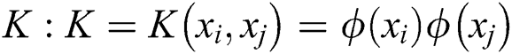 , kernel function matrix.
The final decision function of LSSVM is:

The kernel function adopts the Gaussian radial basis kernel function and is expressed as:

3 PSO-LSSVM Model Based on PCA
The PSO algorithm is used to determine the optimal solution of the key parameters  and
and  of LSSVM and build the PCA-PSO-LSSVM highway engineering cost prediction model. The specific flow chart is shown in Fig. 1.

Figure 1: Flow chart of PCA-PSO-LSSVM model implementation
The steps, which are based on the PCA-PSO-LSSVM model, are presented as follows:
Step 1: Sort and collect samples and perform systematic cluster and principal component analyses on the data.
Step 2: Initialize the particle swarm. The regularization parameter  and the kernel function width coefficient
  in the LSSVM model must be optimized. Set the value range of
  given that the number of particle swarms
  , the maximum number of iteration
  , learning factors
  and
and  , and inertial weighting factors
  and
and  . Generate the first-generation particle swarm randomly.
Step 3: Train the generated parameter combinations of each generation  and
and  as the parameters of the LSSVM model. Calculate the fitness value of each particle swarm generation through the fitness function, and select the root mean square error (MSE) as the function to evaluate the fitness of the particles.
Step 4: Compare the current fitness value  of each particle with the fitness value
  of the historical optimal position. If
 , then update
  . Compare the fitness value
  of the optimal position of each particle with the optimal position fitness value
  of the entire particle swarm. If
 , then update
  . Continue these steps until the optimal solution combination is achieved.
Step 5: Construct the PCA-PSO-LSSVM training model, the fitness graph, and the sample regression curve figure.
Step 6: Input the test sample and obtain the prediction result.
4.1 Selection of Model Evaluation Indicators
Sorting out and collecting 60 groups of highway data in different regions, the main factors that affect highway project cost, namely, main route mileage  , subgrade width
  , subgrade earthwork volume
  , number of bridges
 , number of interchanges
  , number of separated interchanges
  , number of tunnels
 , pavement form
  , landform features
  , and area
  . The predicted value refers to the highway engineering cost per kilometer:
  . The pavement form is determined according to different pavement forms, landform characteristics, and the degree of influence of the area on the construction cost of expressway. The values 0.8 and 0.6 represent the asphalt and cement concrete pavements, respectively. The geomorphic features are presented as follows: 0.2 represents plain and hilly area, 0.5 represents heavy hill area, and 0.8 represents mountainous area. Weighted summation is used when different sections of a road have diverse geomorphic features. In the region, China’s provinces are divided into I, II, and III taking 0.3, 0.6, and 0.9, respectively.
First, hierarchical cluster analysis is used to classify the samples, and several projects with higher similarity can be selected to improve prediction accuracy. A total of 60 groups of highway engineering data are standardized in the SPSS software (Tab. 1). The clustering method selects clustering between groups, and the measurement interval uses square European clustering.
Table 1: Standardization of original data of highway construction
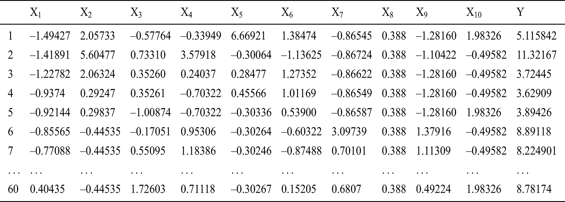
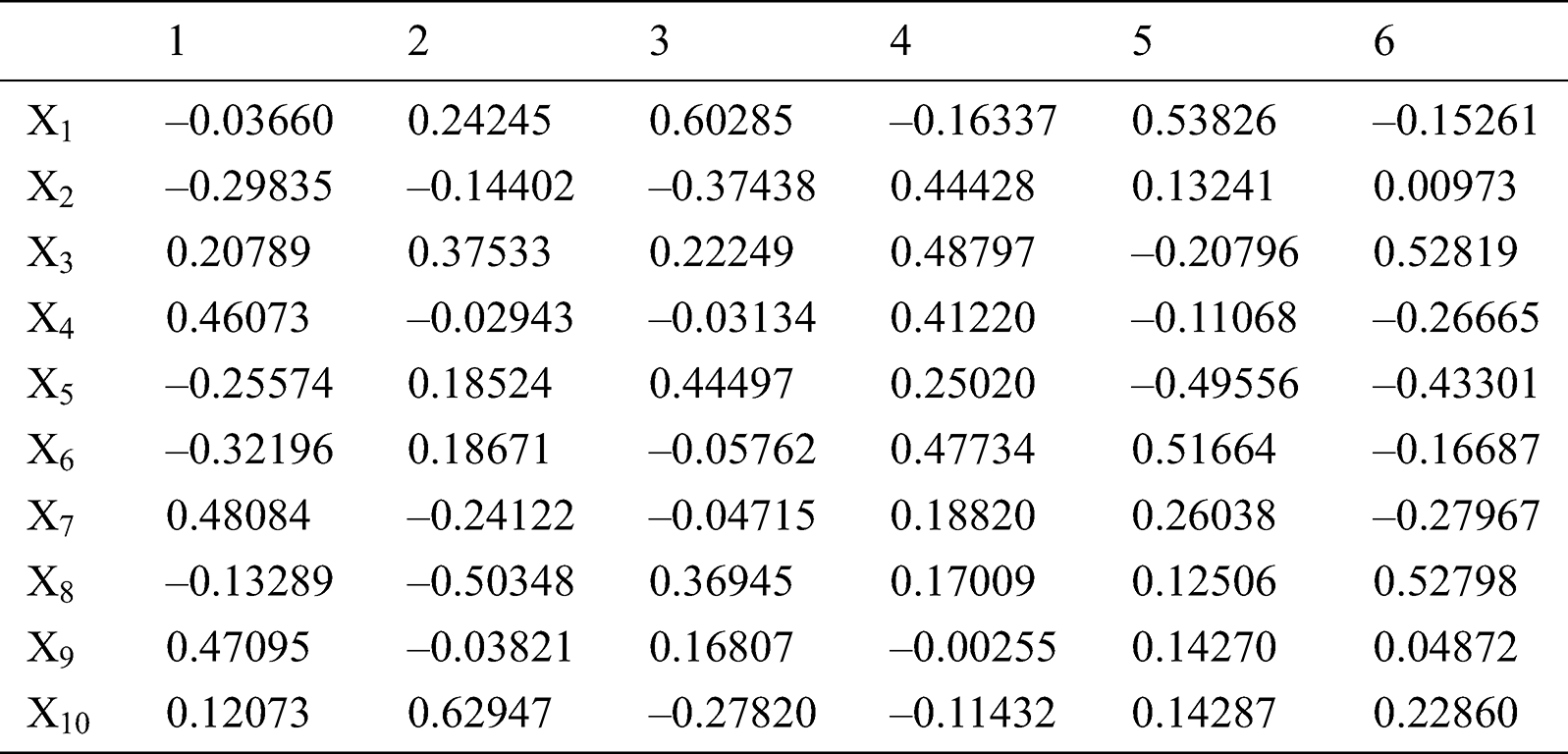
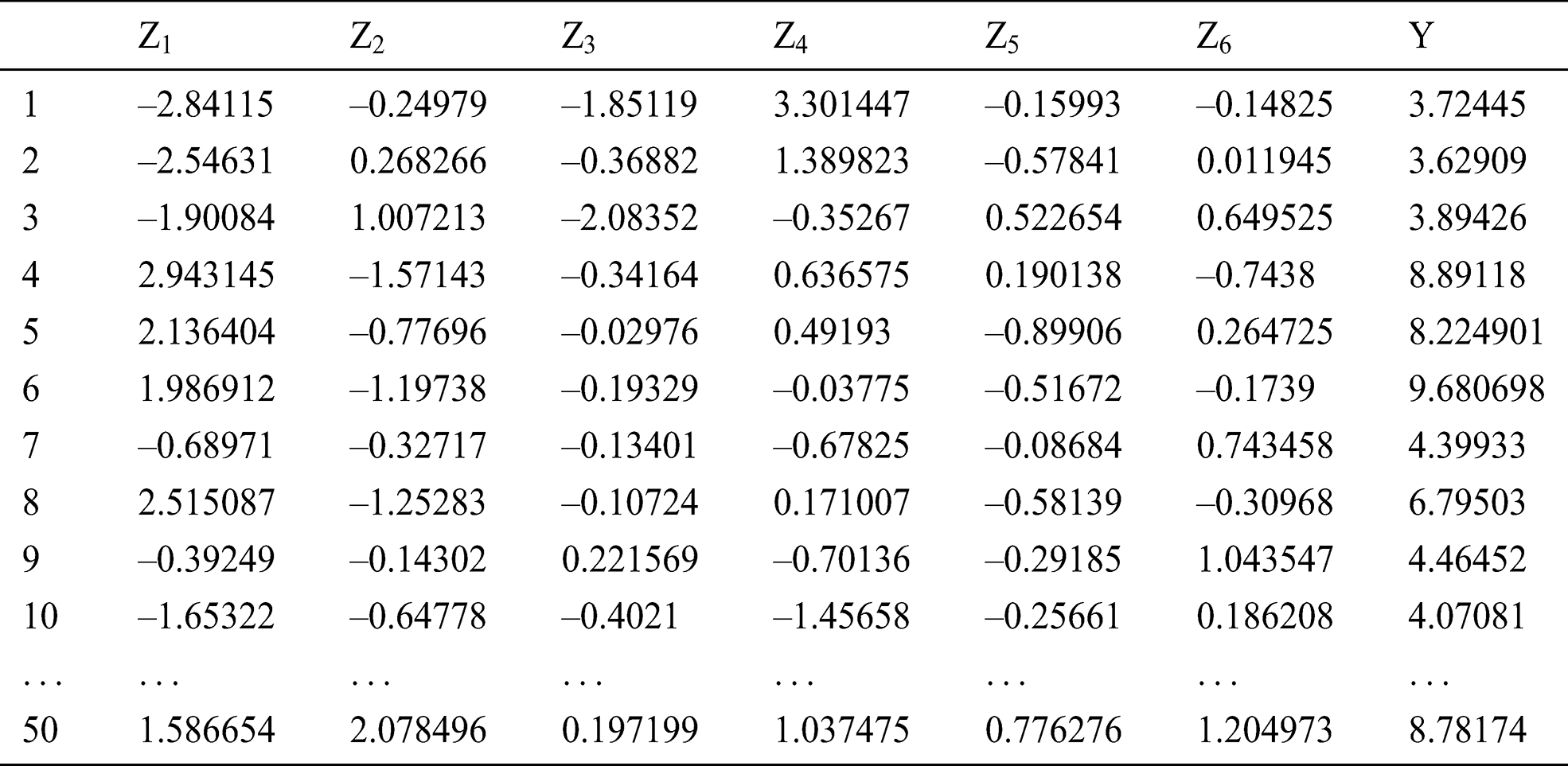
After hierarchical cluster analysis, the 10 sets of data (e.g., 1, 2, 43, 15, 29, 23, 28, 27, 36, and 16) were screened out, and the remaining 50 sets of data were standardized to obtain the data in Tab. 2. The characteristic value and cumulative contribution rate of each component were obtained through PCA (Tab. 3). The first 6 factors with a cumulative contribution rate of 85% were selected as the new principal components. The coefficient matrix (Tab. 4) is acquired according to the  . Finally, by using formula
  and so on, the input sample matrix is obtained (Tab. 5).
Table 2: Standardization sample data

Table 3: Eigenvalue, contribution rate, and cumulative contribution rate

4.3 PCA-PSO-LSSVM Prediction Model
The PCA-PSO-LSSVM prediction model is established using the MATLAB2016(a) simulation platform, and the initialization parameters of the prediction model are set as follows: population size  , maximum number of iterations
  , learning factor
  , inertia weight coefficient
  , regularization parameters
  , and kernel function width coefficient
  . The first 40 groups of the input sample data are applied as the training samples to exercise and learn the PCA-PSO-LSSVM model, and the last 10 groups are utilized as the test samples for prediction. The output is the cost of highway engineering per kilometer/10 million yuan. The fitness curve of the PCA-PSO-LSSVM model is shown in Fig. 2.

Figure 2: Fitness function diagram
Fig. 2 shows that the fitness curves have reached a stable state when the number of iterations reaches 210. The optimal parameter combination of the prediction model is  , and the average relative error of the training sample is
 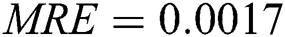 . The sample regression curve with good fitting effect is shown in Fig. 3.

Figure 3: Regression curve of highway engineering cost training sample
4.4 Comparative Analysis with BP neural network and LSSVM model
The regression fitting of the training samples proves that the PCA-PSO-LSSVM model has good learning ability. To verify whether the model also has excellent generalization ability, the prediction is performed by inputting 10 sets of test sample data and by comparing them with the unoptimized LSSVM model and BP neural network model (Fig. 4).

Figure 4: Forecast results of highway engineering cost by different models
Preliminarily, Fig. 4 shows that the effect of the PCA-PSO-LSSVM model prediction is better than those of the BP neural network and the LSSVM model, which have values closest to the actual one. To verify the superiority of the PCA-PSO-LSSVM model more intuitively, the average relative error (MRE) and root mean square relative error (RMSE) are calculated to evaluate the performance of the model (Tabs. 6 and 7, respectively).
Table 6: Comparison of the relative errors of the three prediction models
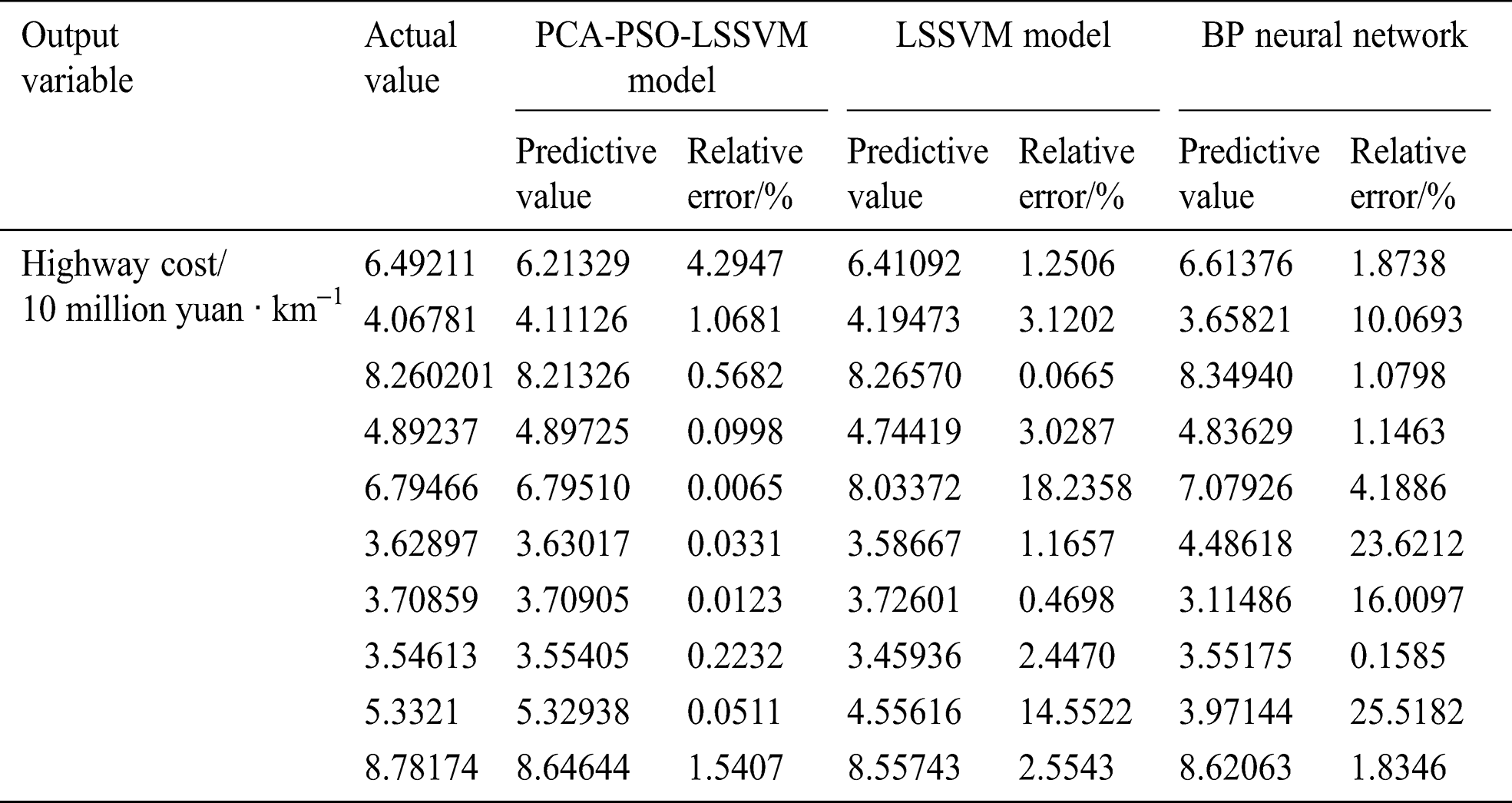
Table 7: Comparison of evaluation indexes of the three models

Tabs. 6 and 7 suggest that the accuracy of the BP neural network for highway project cost prediction is poor with an average relative error and root mean square relative error of 8.55% and 56.92%, respectively. The reason is that the BP neural network needs to rely on large sample data, which have poor generalization ability for small sample learning. Meanwhile, the average relative error and root mean square relative error of the unoptimized LSSVM model are 4.69% and 47.35%, which are more accurate than the BP neural network prediction. The PCA-PSO-LSSVM model has an average relative error and root mean square relative error of 0.79% and 10.01%, respectively. Through comparative analysis, the MRE and RMSE of the PCA-PSO-LSSVM model are the smallest. Thus, this model can predict the cost of highway engineering more accurately.
Based on the principal component analysis method, the least squares support vector machine prediction model is established. It combined with the PSO algorithm to optimize the regularization parameter  and the kernel function width coefficient
  in LSSVM. Overcome the fact that the traditional LSSVM model determines the parameters through experience, thereby resulting in a lower prediction accuracy.
Through the predictive analysis of highway engineering, the PCA-PSO-LSSVM model has the average relative error of 0.79% and the root mean square relative error of 10.01%. Compared with the BP neural network and the unoptimized LSSVM model, the PCA-PSO-LSSVM model has better learning generalization ability and prediction accuracy.
Funding Statement: The authors received no specific funding for this study.
Conflicts of Interest: The authors declare that they have no conflicts of interest to report regarding the present study.
1. A. Ashworth and M. Skitmore. (1982). “Accuracy in estimating chartered quantity surveyor,” London. [Google Scholar]
2. A. H. Boussahaine and T. M. S. Elhag. (1999). “Tender price estimation using ANN methods,” Research Rep. No. 3 School of Architecture. [Google Scholar]
3. J. X. Yang and H. Y. Xie. (2007). “The application of fuzzy neural network in highway engineering cost estimation,” Journal of China & Foreign Highway, vol. 27, no. 5, pp. 16–19. [Google Scholar]
4. H. K. Duan, “Research on highway engineering cost forecast model based on GN-BP,” New Technology and New Process, no. 3, pp. 28–31, 2017. [Google Scholar]
5. Y. H. Pan, Y. L. Zhang and Y. J. Cai. (2016). “Research on highway engineering cost estimation based on GA-BP algorithm,” Journal of Chongqing Jiaotong University (Natural Science Edition), vol. 35, no. 2, pp. 141–145. [Google Scholar]
6. Y. E. Geng, “Analysis of the influencing factors and relationship of highway engineering cost based on system dynamics,” Jiangxi Building Materials, no. 5, pp. 112–114, 2015. [Google Scholar]
7. C. X. Jiang. (2015). “Research on cost control of large real estate companies based on big data,” M.S. dissertation, University of Shandong Jianzhu, Jinan. [Google Scholar]
8. R. Wang, “Determination of influencing factors for road cost prediction based on extended BP network,” Shandong Transportation Science and Technology, no. 3, pp. 29–31, 2019. [Google Scholar]
9. S. Wang. (2017). “Research on construction cost prediction based on particle swarm optimization least square support vector machine,” M.S. dissertation, Qingdao University of Science and Technology, Qingdao. [Google Scholar]
10. Z. Liu, B. Xiang, Y. Q. Song, H. Lu and Q. F. Liu. (2019). “An improved unsupervised image segmentation method based on multi-objective particle swarm optimization clustering algorithm,” Computers, Materials & Continua, vol. 58, no. 2, pp. 451–461. [Google Scholar]
11. S. C. Feng, L. S. Shao and W. J. Lu, “Application of PCA-PSO-LSSVM model in gas emission prediction,’ Journal of Liaoning Technical University (Natural Science Edition), vol. 38, no. 2, pp. 124–129, 2019. [Google Scholar]
12. C. S. Yuan, X. T. Li, Q. M. Jonathan Wu, J. Li and X. M. Sun. (2017). “Fingerprint liveness detection from different fingerprint materials using convolutional neural network and principal component analysis,” Computers, Materials & Continua, vol. 53, no. 4, pp. 357–372. [Google Scholar]
13. Y. Yang. (2020). “Establishment of PSO-LSSVM based on distribution network project cost forecast model and its error analysis,” Automation Technology and Application, vol. 39, no. 2, pp. 98–102. [Google Scholar]
 | This work is licensed under a Creative Commons Attribution 4.0 International License, which permits unrestricted use, distribution, and reproduction in any medium, provided the original work is properly cited. |