DOI:10.32604/csse.2021.014234
| Computer Systems Science & Engineering DOI:10.32604/csse.2021.014234 | |
| Article |
A Quantum Spatial Graph Convolutional Network for Text Classification
1College of Computer Science and Technology, Dalian University of Technology, Dalian, 116024, China
2Department of Computing, University of Worcester, UK
3Department of Information Engineering, Chang’an University, Xi’an, 710054, China
4Department of Cell Biology and Genetics, Shantou University Medical College, Shantou, 515041, China
5Electrical and Computer Engineering Department, COMSATS University Islamabad, Lahore Campus, Pakistan
6School of Information & Communication Engineering Dalian University of Technology, Dalian, 116024, China
7Electrical and Computer Engineering Department, COMSATS University Islamabad, Sahiwal Campus, Pakistan
*Corresponding Author: Hongwei Ge. Email: hwge@dlut.edu.cn
Received: 08 September 2020; Accepted: 08 November 2020
Abstract: The data generated from non-Euclidean domains and its graphical representation (with complex-relationship object interdependence) applications has observed an exponential growth. The sophistication of graph data has posed consequential obstacles to the existing machine learning algorithms. In this study, we have considered a revamped version of a semi-supervised learning algorithm for graph-structured data to address the issue of expanding deep learning approaches to represent the graph data. Additionally, the quantum information theory has been applied through Graph Neural Networks (GNNs) to generate Riemannian metrics in closed-form of several graph layers. In further, to pre-process the adjacency matrix of graphs, a new formulation is established to incorporate high order proximities. The proposed scheme has shown outstanding improvements to overcome the deficiencies in Graph Convolutional Network (GCN), particularly, the information loss and imprecise information representation with acceptable computational overhead. Moreover, the proposed Quantum Graph Convolutional Network (QGCN) has significantly strengthened the GCN on semi-supervised node classification tasks. In parallel, it expands the generalization process with a significant difference by making small random perturbations  of the graph during the training process. The evaluation results are provided on three benchmark datasets, including Citeseer, Cora, and PubMed, that distinctly delineate the superiority of the proposed model in terms of computational accuracy against state-of-the-art GCN and three other methods based on the same algorithms in the existing literature.
Keywords: Text classification; deep learning; graph convolutional networks; semi-supervised learning; GPUs; performance improvements
Text classification (TC) is an imperative process of Natural Language Processing (NLP) to categorize the unstructured textual data into a structured format. At present, TC has numerous applications in various domains, such as news filtering [1], spam detection [2–4], opinion mining [5–8], document organization, and retrieval [9,10]. TC is a widely studied subject in the field of information science and has been important since the beginning of digital text documents. The TC process can be divided into two phases i.e., preprocessing and classification [11]. The preprocessing transforms the text data into valuable features, as this step is important before the classification; in the next phase, classification has been applied to predict a classifier. A model has been built on the grounds of labeled training data and this model will predict the label of previously unlabeled test data. Feature selection and text representation are the two substantive steps in every TC task [12,13]. Conventionally, two prominent techniques are used to represent text data, i.e., bag-of-words (BoW) [14–17] and n-grams [18,19]. In the earlier mentioned technique, a text document has been presented as a set of words with their corresponding frequencies in a document, while in the latter one, the sequence of data elements is found in a more extensive chain of data elements. In the context of the text, an n-gram is the sequence of n words or n characters, where n is an integer greater than zero. In the frame of reference for language comparison, an n-gram is a sequence of characters.
The recent progress in the domain of deep learning has offered promising avenues for researchers. Numerous Deep-Learning based methods emerged for TC. The existing reports indicated that the Deep Neural Networks (DNNs) exceptionally outperform with less demand for engineered features. DNNs can mainly classify into two categories based on hierarchical (e.g., Convolutional Neural Networks (CNN’s) [20–25]) and sequential (e.g., Recurrent neural networks (RNNs)) structures. The RNNs are further defined into more categories, such as Long short-term memory (LSTM) [26–28] and Gated Recurrent Unit (GRU) [29] based on gating mechanisms.
The evidence from respective cohort studies indicated that various text data retain the complex relationship, which can assist in improving classification accuracy for instance, a citation network where articles are linked via citationship. Hence, for better classification results, some graph-based algorithms can efficiently be employed to enjoy the perk of the link’s information [18,30]. One of the pioneering works had been undertaken in 2013 by Bruna et al. [31], a purposing model utilizes spectral graph theory to develop a variant of graph convolution. Starting, thereby, a broad spectrum has been observed in the development and extension of GNNs [20–22]. The research discussed in this article contributes to the prior experimentation done by Kipf et al. [32]. The main contributions of this study are as follows:
• The proposed method overcomes the shortcomings of previous work, with acceptable computational overhead.
• The proposed method can significantly strengthen the semi-supervised node classification task and expand the generalization process with significant differences.
• The QGCN scaffold the quantum information theory with GCN to generate Riemannian metrics to preprocess the adjacency matrix of graphs.
This paper is structured into five sections: The first section gives a brief introduction to TC. The second section examines the earlier endeavors towards TC. In the third section, a new methodology is proposed with schematic illustration, and the processing of the proposed model has been explained with the empirical demonstration. The fourth section is followed by the results obtained using the proposed QGCN, and their comparison with previous models such as GCN, GCNT, Fisher GCN, and Fisher GCNT. Lastly, summarized the main findings and conclusions.
The TC problem has been extensively addressed and implemented in various NLP domains, including databases, information collection, and data mining. In a TC problem: the analysis contains training data  per-labeled with a class
  . The task now is to train a classification model that can predict the appropriate class for an unknown entity
  , which can assign one or more class labels for
  [30,33]. The ultimate objective of TC is to train a classifier for predefined categories and enable it to predict the unknown entities [34]. Formally, we can define TC as a process of sorting documents/texts into single/multiple classes, as specified by their genre [35]. TC can mainly be categorized into two broad categories; single-label and multilabel documents. A single-label document relates to one class, whereas a multilabel document can have multiple classes.
2.2 Graph Convolutional Neural Networks
The existing studies under the umbrella of GNNs are derived from the seminal work of Gorei et al. [36] Furthermore, expounded by Micheli [37] and Scarselli et al. [38]. Numerous initial studies have utilized recurrent neural architectures to investigate the representation of a node of a target by disseminating neighborhood information. CNN’s in the domain of computer vision was the inspiration behind the GCNs. In the past few years, various new techniques emerged to address graph phenomena. Spectral graph theory, as stated by Bruna et al. [31] presented the first prominent research on GCNs.
In the graph, Graph embedding [39,40] is used to capture structural similarities. Deep walk [39] makes the most of the simulation localized walks in the vicinity of the node that is then transmitted to the neural network for language modeling to build the node background. Node2Vec [41] interplays breadth and depth-first sampling techniques to combine and investigate the various neighborhood types.
Monti et al. [40] spread the concept of coordinates of space via learning a series of Gaussian function parameters corresponding to a certain distance towards the embedding of the node. Graph attention networks (GAT) can learn these weights through a mechanism of self-attention. Jumping knowledge networks (JKNets) [42] often concentrate on the node locality concept. JK-Nets experiments show that the notion of subgraph neighborhood varies depending on the graph topology, e.g., random walks advance at nonuniform variance in various graphs. Hence, JK − Nets aggregates across different neighborhoods and takes into account multiple node localities.
2.3 Quantum Fisher Information Matrix
The Quantum information matrix (QIM) is a central aspect in the speculative quantum computation since Cramér-Rao quantum bonds are quite effective when it comes to estimating quantum parameters. After the explosive growth initiated, quantum technology is not theoretical, but technology and has now reached every race of modern life and science. A quantic mechanism technique is referred to as the quantum technique and is intended to create new techniques or enhance current technology in conjunction with quantum resources/phenomena/effects.
Across both theoretical and practical fields, a range of features of quantum technology demonstrated a prodigious impact across leading the next industrial revolution, such as quantum computation, quantum communication, quantum metrology, and quantum cryptography. In the nearish term, quantum metrology has been proven to be an evolving source of practical implications among such techniques.
Quantum metrology is the analysis of high-resolution measurements of physical parameters with high sensitiveness, employing quantum theories to understand physical structures, in particular using quantum entanglement and quantum compression. This area is expected to emerge with more precise measuring technology than the conventional measuring technology.
Both quantum metrology and Cramér-Rao bound use the estimation of quantum parameters, and it is evident that both methods are well-researched mathematical means of estimating the quantum parameter. In quantum Cramer-Rao, the quantum Fisher information and the Quantum fisher information matrix (QFIM) are the principal elements for one-parameter and multiparameter estimates [43].
In addition to quantum metrology, QFIM also interacts with other aspects of quantum physics, such as quantum phase and entanglement witnesses [44,45].
The QFIM also links to other main quantities, such as the quantum geometric tensor [46]. Therefore, a separate evaluation for QFIM in quantum mechanics should be rendered because of the main value of quantum parameter estimation. QFIM calculation techniques have evolved rapidly in various scenarios and models in recent years. However, these methods are not structurally outlined by the community.
Let the vector variable  with
with  the
the  component.
  is encoded in the density matrix
  QFIM is represented as
  , and entry of
  implies as [44–46]

where  symbolizes the anti-commutation and
  is symmetric logarithmic (SLD) parameter derivative
  , described by the equation
  .
.

The symmetric logarithmic derivative (SLD) is a Hermit operator with the average value  by using the above equation,
  can also be explained by Fujiwara et al. [45].

Based on Eq. (1), the sloping input of QFIM is:

That is precisely the parameter of  for QFI. The Fisher Information Matrix (FIM) concept was derived from traditional statistics. For the distribution of probability
  where
where  is the conditional probability for the outcome
  , concerning variable x an entry of FIM is presented as

For discrete outcome results:

As the metrology develops, with the development of quantum metrology [47], the classical probability distribution related FIM is usually denoted as Classical Fisher Information Matrix (CFIM), and its diagonal components are called Classical fisher information (CFI). There is no doubt in the quantum mechanical situation that the measurement method adopted would hardly influence the probability distribution and so to CFIM. This fact indicates the CFIM is a function of measurement. However, QFI is obtained until the optimized measurements are made [5], i.e.,  where
where  represents a positive-operator valued measure (POVM); usually, all the available methods lack in estimating QFIM. The SLD based QFIM is one of the numerous quantum variants of CFIM. The best-suited ones are those containing logarithmic derivatives on either the left or right side.
The SLD-based QFIM is not the only CFIM quantum version. Another well-used ones are centered on logarithmic derivatives from the right and left [48], defined by  , with the corresponding QFIM
  . On the contrary to the SLD based quantum variant, the QFIM are complex with hemitian matrix. QFIMs of all the types fall under a family of Riemannian monotone metrics, as stated by Petz et al. [49] in
  . Generally speaking, all QFIMs lead to Cramér-Rao bound version but with different achievability. For example, D-invariant, which is based on the right algorithmic derivative approaches the goal of bound. Unlike SLD-based, which are real symmetrical, the QFIM is complex and Hermitian oriented on the left and right logarithmic derivatives. All QFIM versions are from a family of monotonous Riemannian metrics generated by Petz [49]. Both QFIMs can provide Cramér-Raobound quantum versions but have different achievements. For example, only the one based on the right logarithmic derivative generates an attainable limit for D-invariant models [50]. For pure states, Fujiwara et al. [45] employed the SLD to a group via
  ; whereas
  is conditionally.
Hermitian, and it will roll back to SLD. A practical example of an antisymmetric logarithmic derivative is the  .
.
The arbitrary size input graph  in
in  is first compared with the prototype graph
  Then
Then  is encoded into a fixed, aligned vertex grid structure, where the vertex orders are preceded by the
  structure. The grid structure of
  is carried through multiple quantum GCN layers to collect multi-scale vertex features, where information on the vertex is propagated among selected vertices after the average mixing matrix. While the GCN layers maintain the original vertex structure orders, the concatenated vertex features form a new grid structure for
  through the graph convolution layers. This grid structure is then moved to a standard CNN layer to learn a classification method. Note that vertex features are displayed in various colors.
The proposed model pipeline is depicted in Fig. 1. two major modules make up the QGCN architecture. The first module is a data handler that collects input data from different sources and preprocesses the data to be passed on to the Quantum GCN module. The QGCN module takes the input graphs and assigns them to the corresponding class labels. Cora, Citeseer, and PubMed are preprocessed weighted datasets that we acquired from Yang et al. [51]. Graph data is the graph metadata of the vertex and the edge, and attributes of the vertex typically contain attributes within each vertex. Then, vector attributes were embedded at the graph vertices. Instead of categorical and text variables, we preprocess every graph data and vertex attribute to translate data to real values, then transfer the attributed weighted graph dataset to the QGCN module. The QGCN module receives the weighted attributed graph data set as input and learns the labeled graph data and distribution of the vertex attributes to classify the labels of the graphs not seen. We transfer the associated weighted graph dataset to the module Quantum GCN. The Quantum GCN module receives the weighted assigned graph dataset as input and prelabeled graph details, and distribution of the vertex attribute to identify the labels of the graphs that are unknown. The Quantum GCN module contains a series of convolution layers followed by a pooling layer based on the specified depth of the proposed neural network followed by a prediction layer. Based on the classification problem, the prediction layer predicts the probability of inputs belonging to the corresponding class labels.
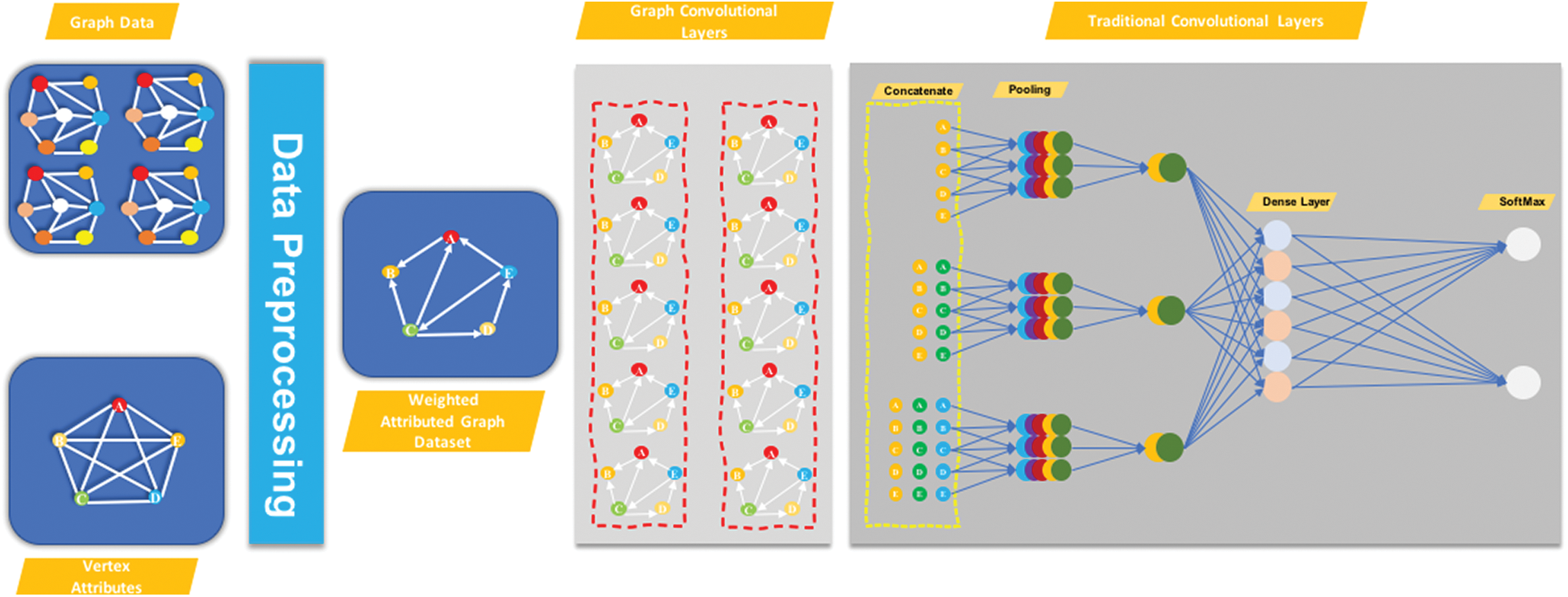
Figure 1: Graphical structure of the proposed model QGCN
As we know, a graph is directly handled by the multi-layered neural network; in other words, the induction of node vectors is positioned as per neighboring properties. Consider a graph  , where sets of nodes are
  , and edges are
  . When node connections are converging, i.e.,
  for any
  . Let
. Let  be a matrix consisting of all
  nodes with their features, where
  is the dimension of the feature vectors, each row
  is the feature vector for
  . We introduce an adjacency matrix
  of
of  and its degree matrix
  , where
  . Because of self-loops, the
  diagonal elements are set to
  . GCN can collect information with only one convolution layer of its immediate neighbors; if several GCN layers are stacked, additional information is integrated. For a one-layer GCN, the new k-dimensional node feature matrix
  is computed as:

where  is the normalized symmetric adjacency matrix and
  is a weight matrix.
  is an activation function, e.g., a
  . Multiple GCN layers assists in reducing higher-order neighborhoods information:

where  denotes the layer number and
  .
.
The objective of learning [48] is to predict those graph perturbations are robust by applying the optimal minimax problem.

Here,  represents the total number of perturbations (e.g.,
  ), which is similar to the GAN training procedure. The Eq. (9) alternatively updates
  along ∇
 , the gradient to
  . Moreover, the optimization problem can be solved by updating alternatively the
  w.r.t. −∇
 . Before proceeding to compute the density matrix and to avoid the numerical instability caused by multiple multiplications,
  matrix should be normalized at first. To compute the correction term like in Eq. (10) to avoid sparse
  term. Moreover,
  contains most of the free parameters. When compared with the GCN, the eigen-decomposition of the sparse needs to be solved once, before training, the eigenvectors multiply the computational cost of training with a factor of
  .
.

That can be resolved in  time effectively. This computation cost can be overlooked if
  is minimal (without increasing the complexity overall),
  computation has the complexity of
  . Where the number of links is
  . Shortly, under similar parameters and complexity, QGCN is slower as compared to GCN. Based on a randomly perturbed graph, the QGCN can be understood as running multiple GCN in parallel, leads to implement our perturbed QGCN.
The main purpose of the proposed research is to present a node-based graph convolution layer to extract multi-scale vertex features and to spread each vertex information progressively towards its nearby vertices and to the vertex itself. This typically requires the transmission of information between each vertex and its surrounding vertices. To extract richer vertex features from the proposed graph convolutional layer, we proposed QIM in terms of the GCN. The design of our proposed model has two sequential stages, firstly the structure and input layer of the grid, secondly the graphic convolution layer in the QIM. In particular, grid structure and input layer maps the arbitrary size graphs to grid structures in a fixed size, along with the aligned vertex grid structures and corresponding vertex matrices of the adjacent matrix, and integrates the matrix structures in the current QGCN model. By propagating vertex information in terms of a QFIM between the aligned grid vertices, the quantum information matrix graph convolution layer further extracts the multi-scale vertex features. Because the extracted vertex features from the graph convolution-layer retain the input grid structure properties, the extracted vertex characteristics can be read, and the graph class can be predicted.
The map graphs of different sizes to the grid structure of fixed-size can be aligned vertices and the related adjacency matrix of the corresponding fixed size. Suppose  represents a set of graphs.
  is a sample graph from
  , with
  representing the vertex set,
  representing the edge set, and
  representing the vertex adjacency matrix. Suppose each vertex
  is represented as a c-dimensional feature vector, the feature information of all
  vertices in
  can be denoted by a
  matrix
  . It should be noted that the row of
  follows the same vertex order of
  . If the graphs in
  are vertex attributed graphs,
  can be the one-hot encoding matrix of the vertex labels.
Sun et al. [52] stated that the canonical parameterization could be derived in a closed-form with the following equation:

However,

A constant scaling of the edge weights results in ds2 = 0 because the density matrix does not vary; hence, either  can be zero or
  , since
  is the density, so it can never be zero, hence,
  ⇒ ρ 6 = 0, G = 0
Now the density matrix can be defined as

Multiplying the above equation by  , we can achieve

By taking derivative, we get

Or it can also be written as

where

Since the result of  is a numerical value, so that we can consider it for our convenient such as

Substituting the value of  from Eq. (12) and the value of
  from Eq. (18) in to Eq. (11) and replacing the indices; such that j = l,k = m,λj = ∆l,λk = ∆m.
We can get our QGCN formulation as below.

where  represent set of documents with labels, and
  is the dimension of the output features, and it is equal to the number of classes,
  represents the label indicator matrix, and to evaluates the performance of our Algorithm, we utilized Gradient descent for training the weight parameters
  and
and  , Gradient descent is an algorithm of optimization to find parameter values (coefficients) of an
  that minimizes a cost function (cost).
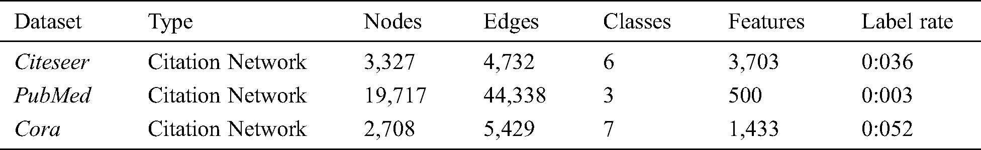
This section evaluates the proposed QGCN model for better classification, even with limited labeled data to determine its performance. Three standard datasets Cora, Citeseer, and PubMed are used to assess the efficiency of the proposed QGCN model. The statistic of different benchmark datasets is shown in Tab. 1 [32]. The Citeseer, PubMed, and Cora datasets with citation network types are also presented. It can be seen that the nodes for Citeseer, PubMed, and Cora are 3227, 197171 and 2708, respectively. The total number of classes are 6, 2 and 7, in Citeseer, PubMed, and Cora, respectively. The values of features are 3703, 500, 1433 for Citeseer, PubMed, and Cora, respectively. Finally, the label rate for Citeseer, PubMed, and Cora is 0:036, 0:003, and 0:052, respectively. Datasets variance has been also enabled to deviate the performance efficiency from the set and expected results.
Table 1: Summary statistics of datasets. As reported in Kipf et al. [32]
We test the efficiency of the proposed QGCN model with four deep learning methods for graphs, including GCN, GCNT, Fisher GCN, and Fisher GCNT [52]. The experiment was conducted on a Core i7 PC with 8 GB RAM and windows 10. We used Python as coding language and TensorFlow for high-performance numerical computation.
An experimental analysis of semi-supervised classification tasks of the transductive node has been conducted. As recently suggested in Monti et al. [40], random training: validation: testing datasets are used, which is based on the same ratios as the Planetoid split as indicated in the “Train: Valid: Test” column of Tab. 1.
We primarily equate GCN that is a state-of-the-art on such datasets and utilized GCNT as a baseline. It was established that random walking similarities would lead to better learning of GNNs [49]. On semi-supervised node classification tasks, preprocessing of the adjacency matrix A can enhance the overall performance of GCN. This procedure is focused on DeepWalk similarities [39].
The GCN codes [32] are adapted to equate the four approaches precisely the same configuration and only differ in matrix  used for the measurement of the graph convolution. As a result of improved perturbation and pre-processing with an enhanced process of generalization, QGCN significantly improves over GCN, GCNT, Fisher GCN, and Fisher GCNT. Additionally, the QGCN provides best performance with both techniques. This variability has been pbserved due to various split of training, validation and testing datasets [40] hence, the scores vary with the split. We have seen a clear development of the approaches introduced over the baselines in repeated experiments.
Tab. 2 validates the proposed QGCN model that significantly outperforms state-of-the-art deep learning methods for graph classifications on the Cora, Citeseer, and PubMed datasets. Here, we have also provided a detailed comparison of the proposed method and its competitors in Figs. 2, 3 and 4.
Table 2: Results comparison with State-of-the-art GCN and its other extensions
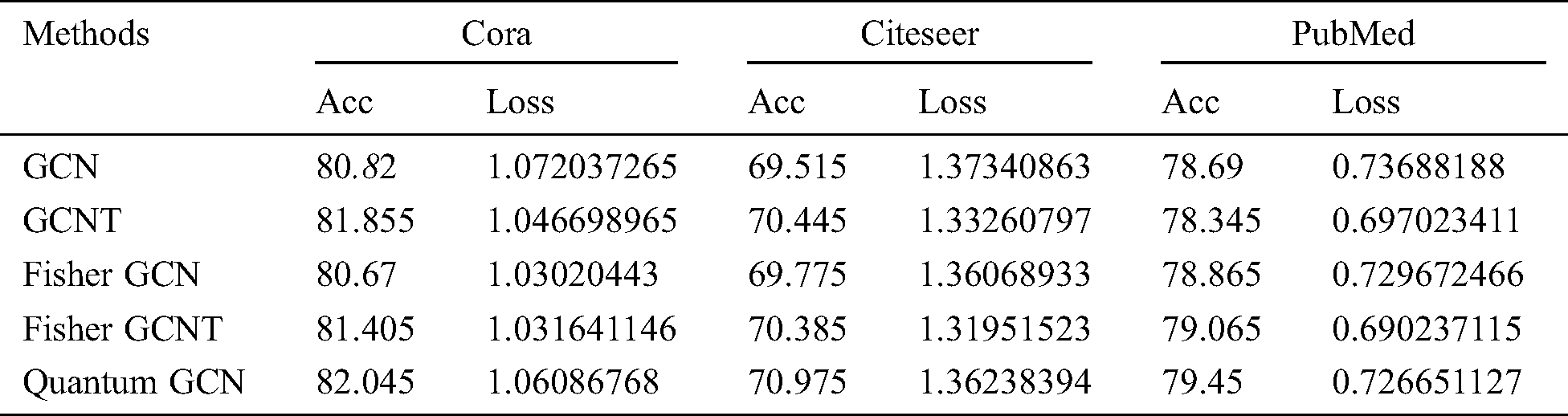
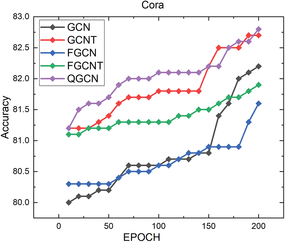
Figure 2: Results on cora dataset
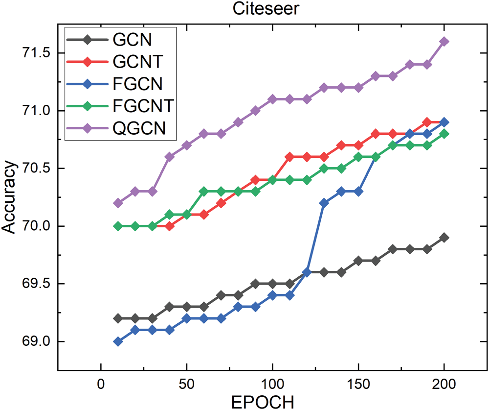
Figure 3: Results on citeseer dataset
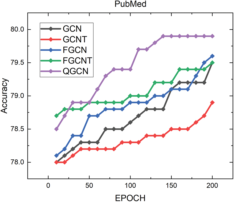
Figure 4: Results on PubMed dataset
The Epoch versus accuracy results on the Cora is shown in Fig. 4. QGCN outperformed from given methods, as shown in Tab. 2. The proposed method shows the best results on the Cora dataset, which is 82.045 as compared to others.
The experimental results on Citeseer are shown in Fig. 3. from comparison: we tested all of the five methods like GCN, GCNT, Fisher GCN, Fisher GCNT, and Quantum GCN for the Citeseer dataset. The GCN showed low performance as compared to Quantum GCN, GCNT, Fisher GCN, and Fisher GCNT. In Tab. 2. it is clear that the proposed QGCN showed high accuracy as compared to other methods, which is 70.975.
The change of accuracy for Epochs on PubMed dataset is shown in Fig. 2. The comparison between GCN, GCNT, Fisher GCN, Fisher GCNT, and Quantum GCN for the PubMed dataset is obtained from the presented Tab. 2. The GCNT showed low performance, where the proposed method again outperformed and showed a high accuracy value, which is 79.45.
This paper proposes a new method, “Quantum GCN”, based on Quantum Information theory and the GCN model for TC. In this proposed work, graph structures are modified in the GCN framework to reveal major improvements in text classification tasks. The overall generalization of the GCN is improved by introducing a new formulation Eq. (19), which is exhibited from quantum information theory. The proposed approach facilitates pre-processing of the GCN graph adjacency matrix to integrate the proximities of a high order. The experimental results are compared with state-of-the-art graph-based methods on three benchmark datasets, namely, Cora, Citeseer, and PubMed Tab. 2. And the proposed method accuracy on the Cora dataset 82.045, Citeseer 70.975, and on PubMed 79.45, which shows superiority over its competitors.
Future work: Our perturbation is efficient enough to add high-order polynomial filters. It would be more beneficial if alternative perturbations based on other distances, e.g., matrix Bregman divergence, can be explored. At the same time, the improved accuracy would broaden the application of the GCN in emerging machine learning processing. Future work will be compromised by comparing various perturbations in the GCN configuration.
Funding Statement: This work was supported by the National Key Research and Development Program of China (2018YFB1600600), the National Natural Science Foundation of China under (61976034, U1808206), and the Dalian Science and Technology Innovation Fund (2019J12GX035).
Conflicts of Interest: The authors declare that they have no conflicts of interest to report regarding the present study.
References
1. L. Douglas Baker and A. K. McCallum. (1998). “Distributional clustering of words for text classification,” in Proc. of the 21st Annual Int. ACM SIGIR Conf. on Research and Development in Information Retrieval, Melbourne, Australia, pp. 96–103.
2. A. Bhowmick and S. M. Hazarika. (2018). “E-mail spam filtering: A review of techniques and trends,” In: Advances in Electronics, Communication and Computing, Springer, Singapore, 583–590.
3. W. Cohen, V. Carvalho and T. Mitchell. (2004). “Learning to classify email into speech acts,” in Proc. of the 2004 Conf. on Empirical Methods in Natural Language Processing, Barcelona, Spain, pp. 309–316.
4. D. D. Lewis and K. A. Knowles. (1997). “Threading electronic mail: A preliminary study,” Information Processing & Management, vol. 33, no. 2, pp. 209–217.
5. H. Chen and D. Zimbra. (2010). “AI and opinion mining,” IEEE Intelligent Systems, vol. 25, no. 3, pp. 74–80.
6. M. S. Hajmohammadi, R. Ibrahim and Z. A. Othman. (2012). “Opinion mining and sentiment analysis: A survey,” International Journal of Computers & Technology, vol. 2, no. 3, pp. 171–178.
7. R. K. Bakshi, N. Kaur, R. Kaur and G. Kaur. (2016). “Opinion mining and sentiment analysis,” In 2016 3rd Int. Conf. on Computing for Sustainable Global Development (INDIACom). New Delhi: IEEE, pp. 452–455.
8. M. Kang, J. Ahn and K. Lee. (2018). “Opinion mining using ensemble text hidden Markov models for text classification,” Expert Systems with Applications, vol. 94, pp. 218–227.
9. S. Chakrabarti, B. Dom, R. Agrawal and P. Raghavan. (1997). “Using taxonomy, discriminants, and signatures for navigating in text databases,” In Int. Conf. on Very Large Data Bases, vol. 97, pp. 446–455.
10. R. A. Naqvi, M. A. Khan, N. Malik, S. Saqib, T. Alyas et al. (2020). , “Roman urdu news headline classification empowered with machine learning,” Computers, Materials & Continua, vol. 65, no. 2, pp. 1221–1236. [Google Scholar]
11. S. Akshay, K. Nayana and S. Karthika. (2015). “A survey on classification and clustering algorithms for uncompressed and compressed text,” International Journal of Applied Engineering Research, vol. 10, no. 10, pp. 27355–27373. [Google Scholar]
12. A. Hotho, A. Nürnberger and G. Paaß. (2005). “A brief survey of text mining,” Journal for Language Technology and Computational Linguistics, vol. 20, pp. 19–62. [Google Scholar]
13. A. Onan and S. Korukoglu. (2016). “A feature selection model based on genetic rank aggregation for text sentiment classification,” Journal of Information Science, vol. 43, no. 1, pp. 25–38. [Google Scholar]
14. A. Dasgupta, P. Drineas, B. Harb, V. Josifovski and M. W. Mahoney. (2007). “Feature selection methods for text classification,” in Proc. of the 13th ACM SIGKDD Int. Conf. on Knowledge Discovery and Data Mining, San Jose, California, USA, pp. 230–239. [Google Scholar]
15. R. E. Fan, K. W. Chang, C. J. Hsieh, X. R. Wang and C. J. Lin. (2008). “Liblinear: A library for large linear classification,” Journal of Machine Learning Research, vol. 9, no. 61, pp. 1871–1874.
16. T. Joachims. (1998). “Text categorization with support vector machines: Learning with many relevant features, ” In European Conf. on Machine Learning, Chemnitz, Germany, pp. 137–142.
17. A. Joulin, E. Grave, P. Bojanowski and T. Mikolov. (2016). “Bag of tricks for efficient text classification,” in Proc. European Chapter of the Association for Computational Linguistics, Valencia, Spain. [Google Scholar]
18. F. B. Silva, R. O. Werneck, S. Goldenstein, S. Tabbone and R. D. Torres. (2018). “Graph-based bag-of-words for classification,” Pattern Recognition, vol. 74, pp. 266–285. [Google Scholar]
19. Y. Luo, A. R. Sohani, E. P. Hochberg and P. Szolovits. (2014). “Automatic lymphoma classification with sentence subgraph mining from pathology reports,” Journal of the American Medical Informatics Association, vol. 21, no. 5, pp. 824–832. [Google Scholar]
20. S. Lai, L. Xu, K. Liu and J. Zhao. (2015). “Recurrent convolutional neural networks for text classification,” in Twenty-ninth AAAI Conf. on Artificial Intelligence, Berlin, Heidelberg, pp. 233–240. [Google Scholar]
21. M. Jaderberg, K. Simonyan, A. Vedaldi and A. Zisserman. (2016). “Reading text in the wild with convolutional neural networks,” International Journal of Computer Vision, vol. 116, no. 1, pp. 1–20.
22. D. Scherer, A. Müller and S. Behnke. (2010). “Evaluation of pooling operations in convolutional architectures for object recognition,” in Int. Conf. on Artificial Neural Networks, Thessaloniki, Greece, pp. 92–101. [Google Scholar]
23. I. Muhammad, W. Liu, A. Jahangir, S. M. Nouman and M. Aparna. (2019). “A novel localization technique using luminous flux,” Applied Sciences, vol. 9, no. 23, pp. 5027. [Google Scholar]
24. M. N. Sohail, R. Jiadong, M. M. Uba, M. Irshad, W. Iqbal et al. (2019). , “A hybrid forecast cost benefit classification of diabetes mellitus prevalence based on epidemiological study on real-life patient’s data,” Scientific Reports, vol. 9, no. 1, pp. 16.
25. Y. Kim. (2014). “Convolutional neural networks for sentence classification,” in Proc. of the 2014 Conf. on Empirical Methods in Natural Language Processing (EMNLPDoha, Qatar, pp. 1746–1751. [Google Scholar]
26. I. Sutskever, J. Martens and G. E. Hinton. (2011). “Generating text with recurrent neural networks,” in Int. Conf. on Machine Learning (ICMLBellevue, WA, USA. [Google Scholar]
27. A. Graves and J. Schmidhuber. (2005). “Framewise phoneme classification with bidirectional long short term memory and other neural network architectures,” Neural Networks, vol. 18, no. 5–6, pp. 602–610. [Google Scholar]
28. P. Liu, X. Qiu and X. Huang. (2016). “Recurrent neural network for text classification with multi-task learning,” in Proc. of Int. Joint Conf. on Artificial Intelligence, Budapest, Hungary. [Google Scholar]
29. M. E. Peters, M. Neumann, M. Iyyer, M. Gardner, C. Clark et al. (2018). , “Deep contextualized word representations,” in Proc. of North American Chapter of the Association for Computational Linguistics, New Orleans, Louisiana. [Google Scholar]
30. J. Zhang, X. Shi, S. Zhao and I. King. (2019). “Star-gcn: Stacked and reconstructed graph convolutional networks for recommender systems,” In Proc. of the twenty-Eighth Int. Joint Conf. on Artificial Intelligence, pp. 4264–4270. [Google Scholar]
31. J. Bruna, W. Zaremba, A. Szlam and Y. LeCun. (2019). “Spectral networks and locally connected networks on graphs,” In Proc. of the twenty-Eighth Int. Joint Conf. on Artificial Intelligence, pp. 4264–4270. [Google Scholar]
32. T. N. Kipf and M. Welling. (2016). “Semi-supervised classification with graph convolutional networks,” Int. Conf. on Learning Representations (ICLRPalais des Congrès Neptune, Toulon, France. [Google Scholar]
33. K. Kowsari, K. Jafari Meimandi, M. Heidarysafa, S. Mendu, L. Barnes et al. (2019). , “Text classification algorithms: A survey,” Information, vol. 10, no. 4, pp. 150. [Google Scholar]
34. F. P. Shah and V. Patel. (2016). “A review on feature selection and feature extraction for text classification,” Int. Conf. on Wireless Communications, Signal Processing and Networking (WiSPNETChennai, India, pp. 2264–2268. [Google Scholar]
35. F. Joseph and N. Ramakrishnan. (2015). “Text categorization using improved k nearest neighbor algorithm,” International Journal of Engineering Trends and Technology, vol. 4, pp. 65–68. [Google Scholar]
36. M. Gori, G. Monfardini and F. Scarselli. (2005). “A new model for learning in graph domains,” In Proc. of IEEE Int. Joint Conf. on Neural Networks, vol. 2, pp. 729–734. [Google Scholar]
37. A. Micheli. (2009). “Neural network for graphs: A contextual constructive approach,” IEEE Transactions on Neural Networks, vol. 20, no. 3, pp. 498–511. [Google Scholar]
38. F. Scarselli, M. Gori, A. C. Tsoi, M. Hagenbuchner and G. Monfardini. (2009). “The graph neural network model,” IEEE Transactions on Neural Networks, vol. 20, no. 1, pp. 61–80. [Google Scholar]
39. B. Perozzi, R. Al-Rfou and S. Skiena. (2014). “Deepwalk: Online learning of social representations,” in Proc. of the 20th ACM SIGKDD Int. Conf. on Knowledge Discovery and Data Mining, New York, USA, pp. 701–710. [Google Scholar]
40. F. Monti, D. Boscaini, J. Masci, E. Rodola, J. Svoboda et al. (2017). , “Geometric deep learning on graphs and manifolds using mixture model cnns,” in Proc. of the IEEE Conf. on Computer Vision and Pattern Recognition, Glasgow, UK, pp. 5115–5124. [Google Scholar]
41. A. Grover and J. Leskovec. (2016). “node2vec: Scalable feature learning for networks,” in Proc. of the 22nd ACM SIGKDD Int. Conf. on Knowledge Discovery and Data Mining, San Fransico, California, pp. 855–864. [Google Scholar]
42. K. Xu, C. Li, Y. Tian, T. Sonobe, K. Kawarabayashi et al., “Representation learning on graphs with jumping knowledge networks,” Int. Conf. on Machine Learning (ICMLVienna, Austria, pp. 5453–5462. [Google Scholar]
43. C. W. Helstrom and C. W. Helstrom. (1976). Quantum detection and estimation theory, vol. 3. New York: Academic press. [Google Scholar]
44. P. Hyllus, W. Laskowski, R. Krischek, C. Schwemmer and W. Wieczorek. (2012). “Fisher information and multiparticle entanglement,” Physical Review A, vol. 85, no. 2, pp. 1. [Google Scholar]
45. A. Fujiwara and H. Nagaoka. (1995). “Quantum fisher metric and estimation for pure state models,” Physics Letters A, vol. 201, no. 2–3, pp. 119–124. [Google Scholar]
46. L. C. Venuti and P. Zanardi. (2007). “Quantum critical scaling of the geometric tensors,” Physical Review Letters, vol. 99, no. 9, pp. 095701. [Google Scholar]
47. G. Tóth. (2012). “Multipartite entanglement and high-precision metrology,” Physical Review A, vol. 85, no. 2, pp. 195. [Google Scholar]
48. H. Yuen and M. Lax. (1973). “Multiple-parameter quantum estimation and measurement of nonselfadjoint observables,” IEEE Transactions on Information Theory, vol. 19, no. 6, pp. 740–750. [Google Scholar]
49. D. Petz. (1996). “Monotone metrics on matrix spaces,” Linear Algebra and its Applications, vol. 244, pp. 81–96. [Google Scholar]
50. J. Suzuki. (2016). “Explicit formula for the Holevo bound for two-parameter qubit-state estimation problem,” Journal of Mathematical Physics, vol. 57, no. 4, pp. 042201. [Google Scholar]
51. Z. Yang, W. Cohen and R. Salakhudinov. (2016). “Revisiting semi-supervised learning with graph embeddings,” in Int. Conf. on Machine Learning, New York City, NY, USA, pp. 40–48. [Google Scholar]
52. K. Sun, P. Koniusz and Z. Wang. (2019). “Fisher-bures adversary graph convolutional networks,” in Proc. of The 35th Uncertainty in Artificial Intelligence Conf., PMLR, Tel Aviv, Israel, pp. 465–475. [Google Scholar]
 | This work is licensed under a Creative Commons Attribution 4.0 International License, which permits unrestricted use, distribution, and reproduction in any medium, provided the original work is properly cited. |