Computer Systems Science & Engineering DOI:10.32604/csse.2021.014334
Article

Optimal Robust Control for Unstable Delay System

Rihem Farkh1,2,*, Khaled A. Aljaloud1, Moufida Ksouri2 and Faouzi Bouani2

1King Saud University, Riyadh, 11451, Saudi Arabia
2Laboratory for Analysis, Conception and Control of Systems, LR-11-ES20, Department of Electrical Engineering, National Engineering School of Tunis, Tunis El Manar University, Tunis, 1002, Tunisia
*Corresponding Author: Rihem Farkh. Email: rfarkh@ksu.edu.sa
Received: 14 September 2020; Accepted: 08 November 2020

Abstract: Proportional-Integral-Derivative control system has been widely used in industrial applications. For uncertain and unstable systems, tuning controller parameters to satisfy the process requirements is very challenging. In general, the whole system’s performance strongly depends on the controller’s efficiency and hence the tuning process plays a key role in the system’s response. This paper presents a robust optimal Proportional-Integral-Derivative controller design methodology for the control of unstable delay system with parametric uncertainty using a combination of Kharitonov theorem and genetic algorithm optimization based approaches. In this study, the Generalized Kharitonov Theorem (GKT) for quasi-polynomials is employed for the purpose of designing a robust controller that can simultaneously stabilize a given unstable second-order interval plant family with time delay. Using a constructive procedure based on the Hermite-Biehler theorem, we obtain all the Proportional-Integral-Derivative gains that stabilize the uncertain and unstable second-order delay system. Genetic Algorithms (GAs) are utilized to optimize the three parameters of the PID controllers and the three parameters of the system which provide the best control that makes the system robust stable under uncertainties. Specifically, the method uses genetic algorithms to determine the optimum parameters by minimizing the integral of time-weighted absolute error ITAE, the Integral-Square-Error ISE, the integral of absolute error IAE and the integral of time-weighted Square-Error ITSE. The validity and relatively effortless application of presented theoretical concepts are demonstrated through a computation and simulation example.

Keywords: Unstable time-delay system; interval plants; generalized Kharitonov theorem; PID controller; Hermite-Biehler theorem; stability region; genetic algorithms; optimum PID controller; optimum system parameters

1  Introduction

Time lags occur often in various engineering systems and industry processes, such as in communication networks, chemical processes, turbojet engines, and hydraulic systems. Delays have a considerable influence on the behavior of the closed-loop systems, can generate oscillations, and even lead to instabilities [1]. Dugard et al. [1] reported that more than 90% of physical systems in process control can be approximated by first- and second-order (about 30%) models with time delay with acceptable accuracy.

Open-loop unstable delay systems are often encountered in process industry, and pose a more challenging problem to controller design compared to that of stable open-loop systems. The presence of an unstable pole in the system imposes a minimum limit on the control performance, which in some cases can lead to an excessive overshoot and long settling time.

Proportional-Integral-Derivative (PID) controller, though a very old design, is still one of the favorite and most widely used controllers for many industrial process control applications. This is due to its simple structure, satisfactory control performance, and acceptable robustness [2]. For systems with long time delay, several methods for determining the PID controller parameters have been developed over the past 60 years. Much attention has focused on stabilizing uncertain systems with or without time delay using PID controllers.

One of the well-known approaches to computing the stabilizing PID controller region is based on a generalization of the Hermite-Biehler theorem [3]. This approach requires sweeping over the proportional gain to find all stabilizing regions of the PID parameters. The Hermite-Biehler theorem has become the basis of an extended theorem used to find the PID stabilizing parameter regions, e.g., in Farkh et al. [4], where the complete stabilizing set of the classical PI and PID controller parameter regions for unstable second-order time-delay plants were derived.

Robust stability of uncertain systems has become of great interest in the past few decades. Robustness is defined as the performance and stability of plants exposed to uncertainties. The Kharitonov theorem is well-known for stability analysis of interval systems. Based on the Kharitonov theorem, the edge theorem in Barmish et al. [5] and the box theorem in Bhattacharyya et al. [6] suggested that the set of transfer functions generated by changing the perturbed coefficients in the prescribed ranges corresponds to a box in the parameter space, which is referred to as “interval plants.” The Generalized Kharitonov Theorem (GKT) reveals that a controller robustly stabilizes the interval system if it stabilizes a prescribed set of line segments in the plant parameter space [6,7].

To determine the robust stability of a time-delay system subjected to parametric uncertainty, researchers have extended the GKT and the edge theorem to quasi-polynomials [6,8,9].

Prior studies have obtained some important results relating to the stabilization of interval systems. Barmish et al. [5] proved that a first-order controller stabilizes an interval plant if and only if it simultaneously stabilizes the 16 plants of the Kharitonov plant family. A parameter plan, based on the gain phase margin tester method and the Kharitonov theorem, was used to obtain a non-constructive region, in which a PID controller stabilizes the entire interval plants [10]. In Tan et al. [11], it is shown that the stability boundary locus can also be exploited to find the stabilizing region of the PI parameters for the control of a plant with uncertain parameters. Patre et al. [12] presented a two-degrees-of-freedom design methodology for interval process plants to guarantee both robust stability and satisfactory performance.

In Ho et al. [13] and Silva et al. [14], the Hermite-Biehler theorem was used for the formulation of P, PI, and PID controllers to stabilize a delay-free interval plant family. In Silva et al. [14], the stabilizing problem of a PI/PID controller for the first-order delay system was analyzed, and then used to obtain all PI and PID gains that stabilize an interval first-order delay system [15].

In this paper, we endeavor to determine the set of all PID gains that stabilize an uncertain and unstable second-order delay system, where the coefficients are subjected to perturbation within prescribed ranges. We propose an approach based on combining the background considerations presented in Section 3 and the result obtained by Farkh et al. [4]. Then, the optimal PID controller parameters and optimal system parameters are determined by applying the optimization method in the robust stable region using the integral performance criteria.

The rest of the paper is organized as follows: In Section 2 we discuss the computation of all PID controllers for an unstable second-order delay system. The problem formulation is given in Section 3. Section 4 is devoted to the robust stabilization problem for an uncertain and unstable second-order system with time delay controlled via a PID controller. Section 5 is reserved for the simulation example. A description and application of the genetic algorithm (GA) is presented in Section 6, and conclusions are presented in Section 7.

2  PID Control for Unstable Second-Order Delay System

In Farkh et al. [4], the computation of all stabilizing PID controllers for an unstable delay system was considered.

2.1 Theorem 1 [4]

Under the assumptions of K > 0, L > 0, a0 < 0 and/or a1 > 0, the values, for which there is a solution to the stabilization problem of the PID controller of an unstable second-order delay system, we verify that:

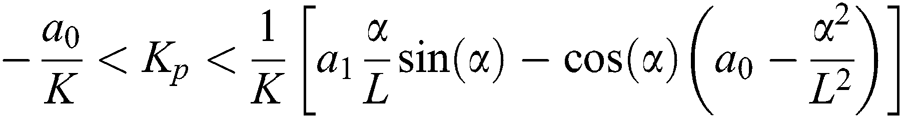
where is the solution to the following equation:

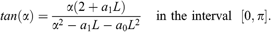
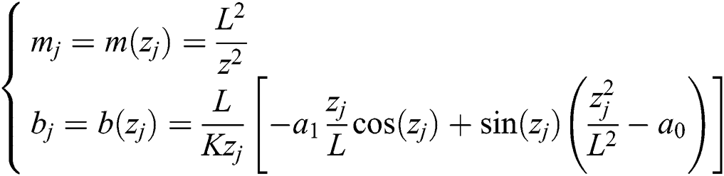
For Kp values outside the above range, there are no stabilizing PID controllers. The complete stabilizing region given by the cross-section of the stabilizing region in the (Ki,Kd)-space is the triangle Δ Fig. 1.

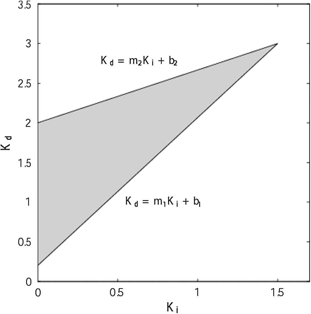
Figure 1: Stabilizing region of (Ki,Kd)-space

The parameters necessary for determining the boundaries, can be obtained using the following equations:

where are the positive-real roots of arranged in ascending order of magnitude, where is expressed by:

2.2 Example

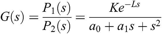
We consider a second-order delay system described by the following transfer function:

To determine the values, we look for in the interval satisfying . The range is given by . The system stability region in the -plane is presented in Fig. 2.

Figure 2: Controller stability domain in -plane for an unstable second-order delay system

3  Robust Controller Design for an Interval Plant with Time Delay

In this section, a procedure is proposed for robust stabilization of an unstable delay system that belongs to a linear interval plant, where the time delay, , is a known constant.

Consider the following transfer function:

where and are linear interval polynomials. Our objective is to find a robust controller, , with the fixed polynomials and to guarantee the robust stability of the system.

We can use the GKT extended for quasi-polynomials [6], to compute all the stabilizing controller parameters for interval systems with a time delay. We review some results from the area of parametric robust control before stating the GKT. Consider the following family of quasi-polynomials :

where is a fixed two-tuple of real interval polynomials. Each is a linear interval polynomial characterized by the intervals as follows:

are real independent interval polynomials defined as:

is a fixed two-tuple of complex quasi-polynomials of the following form:

with the being complex polynomials satisfying the following condition:

In our case, we use with a single delay: .

According to Bhattacharyya et al. [6], the stability problem of Eq. (2) can be solved with the GKT by constructing an extremal set of line segments, , where the stability of implies the stability of . will be generated by constructing an extremal subset , using the Kharitonov polynomials of .

3.1 Theorem 2 [6]

Let be a given two-tuple of complex quasi-polynomials satisfying the condition of Eq. (6), and let be an independent real interval polynomial. stabilizes the entire family if and only if stabilizes every two-tuple segment in . Equivalently, is stable if and only if is stable.

3.2 Corollary

stabilizes the linear system if and only if the controller stabilizes the extremal transfer function discussed in detail later.

The GKT, we first need to determine the extremal set of line segments, . From the segment polynomials of and , eight Kharitonov vertex equations are obtained as follows [6,16]:

and

where

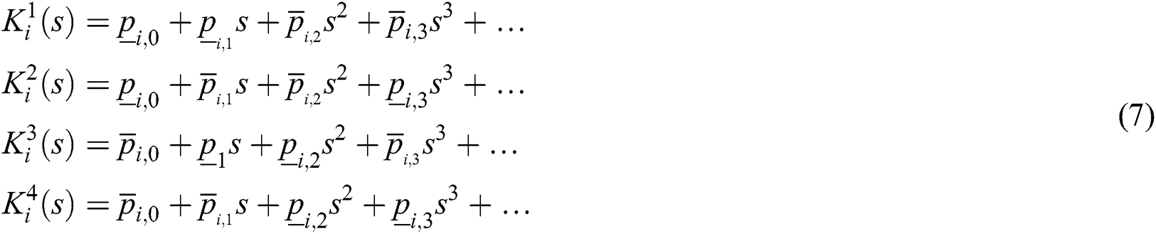
The extremal subset 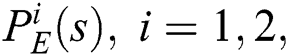consists of [3]:

where , , and . In the above equation, the number of extremal equations is , where indicates the number of perturbed polynomials, and the connection points to make the Kharitonov polytope .

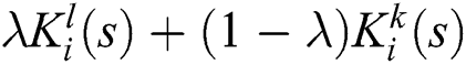Some of the subset equations may be the same, hence, the extremal subset is defined as [6]:

The extremal subset of line segments (or generalized Kharitonov segment polynomials) is [6]:

where

With the knowledge that , if all polynomials of the linear interval system are stable, the system with perturbed parameters will also be stable.

The previous results of the robust parametric approach control proved to be an efficient control design technique. In the following, they will be used for the synthesis controllers that simultaneously stabilize a given uncertain time-delay system.

4  Robust PID Stabilization for an Uncertain and Unstable Second-Order Time-Delay System

In this section, we consider the problem of characterizing all PID controllers that stabilize a given unstable second-order interval plant with a time delay:

where , , and . The controller is given by .

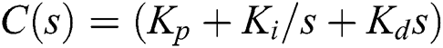To obtain all PID gains that stabilize using the GKT for quasi-polynomials, we consider a new transfer function as follows:

and the compensator as follows:

The family of closed-loop characteristic quasi-polynomials becomes:

The problem of characterizing all stabilizing PID controllers requires determining all the values of , , and for which the entire family of closed-loop characteristic quasi-polynomials is stable. Let and be the Kharitonov polynomials corresponding to and , respectively, where , , and .

Let denote the family of 32 plant segments:

Then, consists of the following plant segments:

where the 32 extremal plants in Eq. (13) are reduced to 20.

The closed-loop characteristic quasi-polynomials for each of these 32 plant segments, , are denoted by and are defined as:

where

We posit the following theorem on stabilizing an unstable second-order interval plant with time delay using a PID controller.

4.1 Theorem 3

Let be an unstable second-order interval plant with uncertain time delay. The entire family is stabilized by a PID controller if and only if each is stabilized by that same PID controller.

4.2 Proof

From Theorem 2, it follows that the entire family is stable if and only if are all stable. Therefore, the entire family is stabilized by a PID controller if and only if every element of is simultaneously stabilized by the same PID.

To obtain a characterization of all PID controllers that stabilize the interval plant by applying this procedure to each belonging to , we will use the results from Farkh et al. [4].

5  Example

We consider the plant family 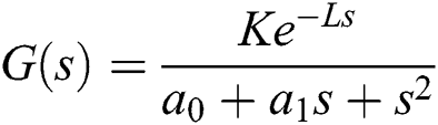, where 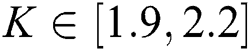, , and .

The entire family is given as follows:

According to from Eq. (14), we obtain:

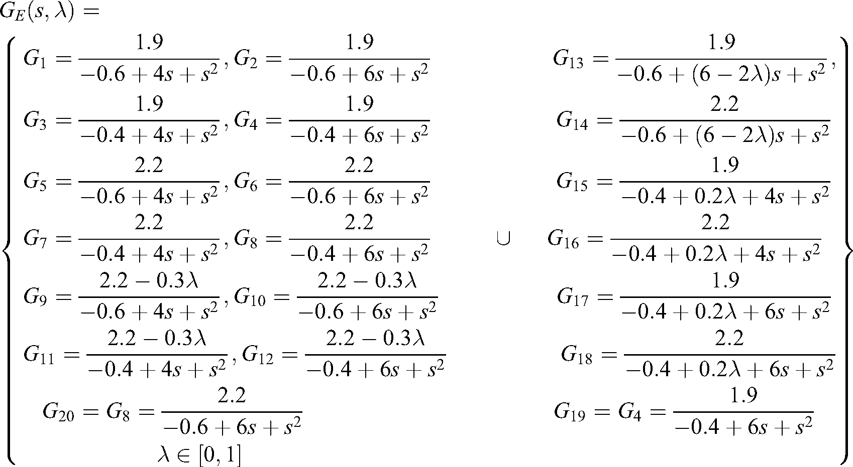
We remark here that from to , we have an infinity of transfer function sets due to their dependence on . To reduce the complexity of the problem, we set to 0, 0.33, 0.66, and 1 as different values of for to , and we also set to 0, 0.25, 0.5, 0.75, and 1 as different values of for to , respectively. Therefore, we obtain:

We define , where for , and , and obtain:

To compute all the stabilizing PID gains, we first determine all the gain stabilizers for :

For a fixed , for instance, , we obtain the stabilizing set of values for by using the result presented in Farkh et al. [4], which is applied to each transfer function belonging to . Fig. 3 presents these stability regions in the -plane.

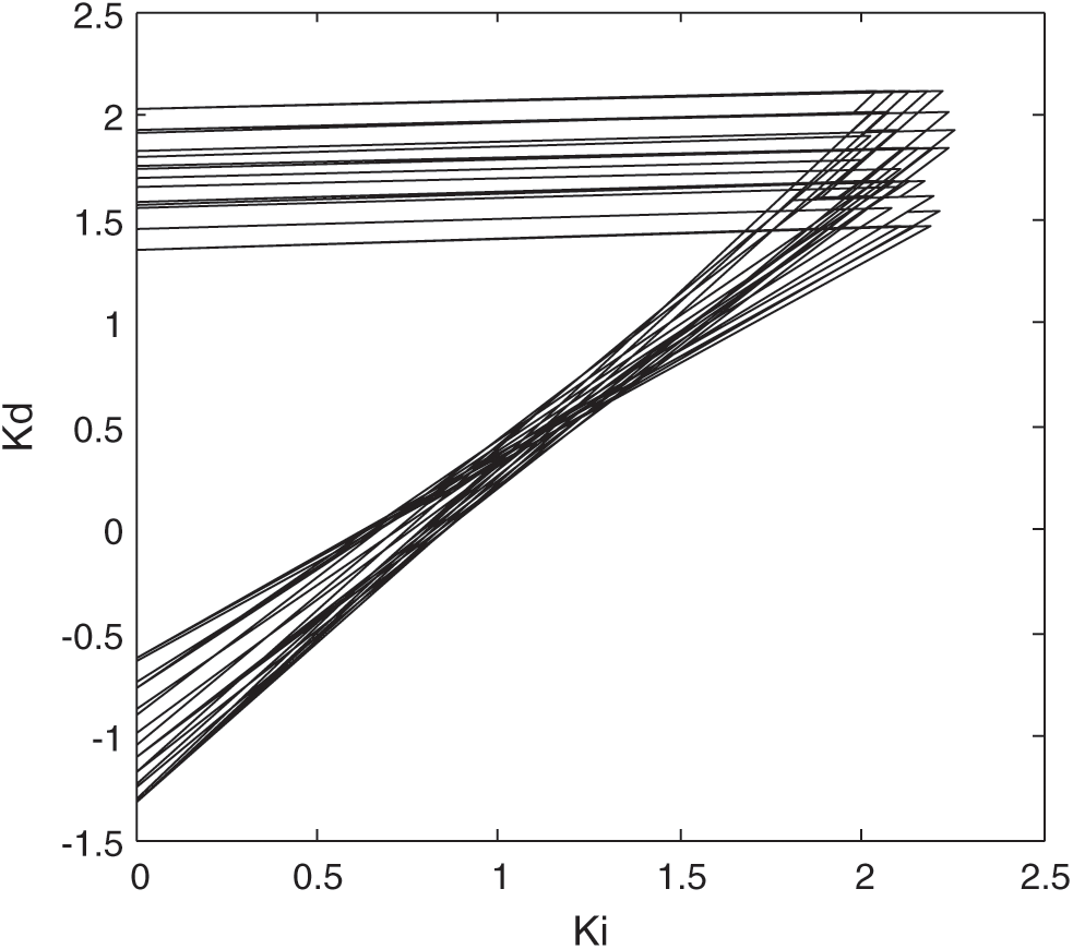
Figure 3: Stabilizing set of for of

The intersection of these stability regions presents an overlapping area of the boundaries constituting the entire feasible controller sets that stabilize the entire family . Fig. 4 presents a zoom-in of Fig. 3.

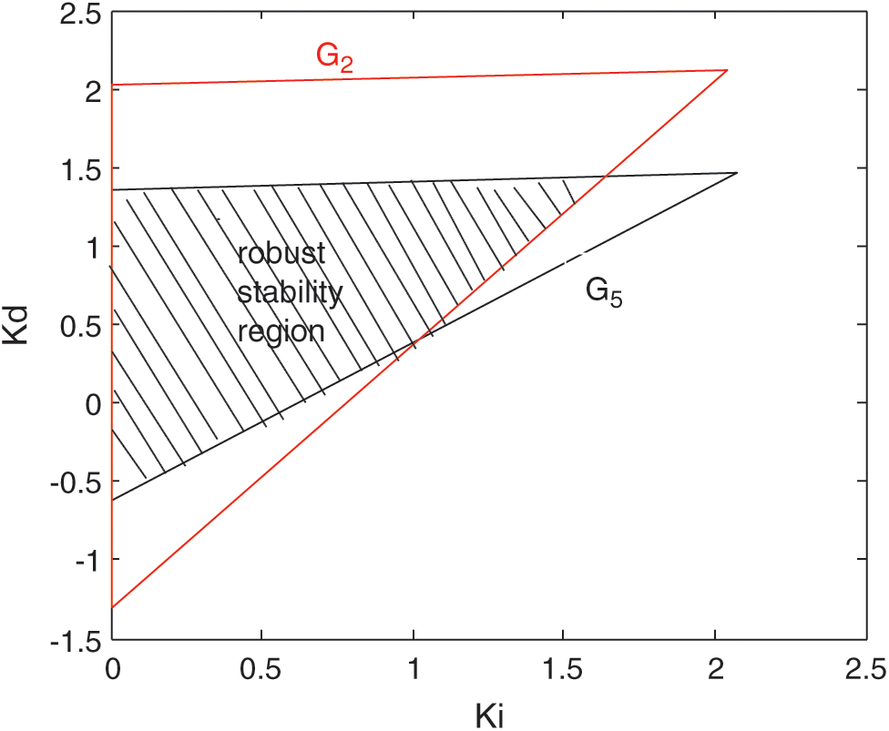
Figure 4: Robust stability region in the -plane for of

Finally, by sweeping over and repeating the above procedure, we obtain all the stabilizing sets of .

6  Optimization

6.1 Genetic Algorithm

GAs are efficient stochastic search methods based on the concepts of natural selection and evolutionary genetics. GAs are communities of individuals, in which through randomizing the cycle of discovery, crossover and mutation, individuals can adjust to a specific setting. The environment offers valuable knowledge (fitness) to individuals, and the selection mechanism supports the preservation of individuals of greater quality. Therefore, during the development cycle, the overall output of the population is growing, ideally contributing to an optimal solution. GAs have been used in diverse fields and are considered as an efficient tool for global optimization. Attempts to apply GAs to control system and identification design problems have been made [16]. Fig. 6 illustrates the theory of GA optimization for control problems.

We look for the optimum system and controller parameters in the robust stability area using one of the following requirements ITAE integral of time-weighted absolute error, ISE Integral-Square-Error, IAE integral of absolute error and ITSE integral of time-weighted Square-Error defined by following relationships:

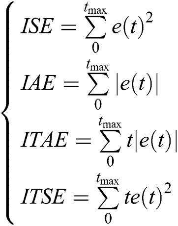
If we want to reduce the tuning energy, the ITAE and IAE criteria should be considered. Conversely, the ITAE and the IAE parameters are being considered when we want to reduce the tuning energy. If we assign preference to rising time, the ITSE criteria are adopted, while we choose the ISE criterion to guarantee the energetic tuning costs [16].

The following algorithm sums up the steps of the control law:

  1.  Introduction of the following parameters:

–    : individual number in each population

–    initial population

–    : generation number

Initialization of the generation counter ()

Initialization of the individual counter ()

For to

efficiency evaluation of jth population individual

Individual counter incrementing ().

–    If , going back to Step 4.

–    Otherwise, application of the genetic operators (selection, crossover, and mutation) for finding a new population.

Generation counter incrementing (),

If , going back to Step 3.

Selecting , , and , which correspond to the best individual in the last population (individual with the highest fitness).

In the following, a GA with the generation number of 100, , , and individual number in each population of 20.

6.2 Example

We consider the uncertain unstable delay system , where , , , and the delay L = 0.5 s.

The robust PID stability region is shown Fig. 5, where it can be seen that , , and population individuals are choosing between , , and . The optimum PID and system parameters provided by GA are presented in Tab. 1.

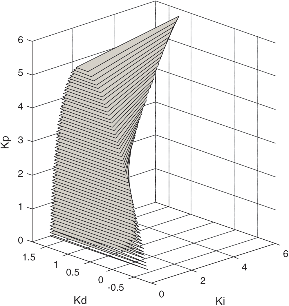
Figure 5: Final robust stability region in -plane for unstable interval plant

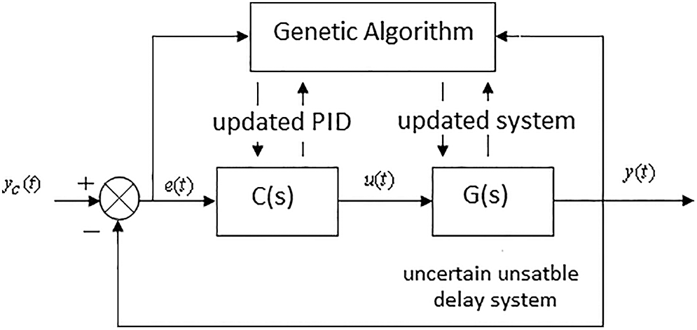
Figure 6: Optimization principle

Table 1: Optimum PID and system parameters

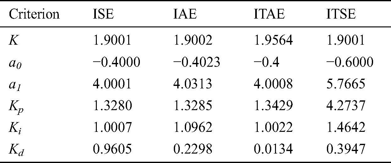
Fig. 7 shows the step responses of the closed-loop system using the values from Tab. 1.

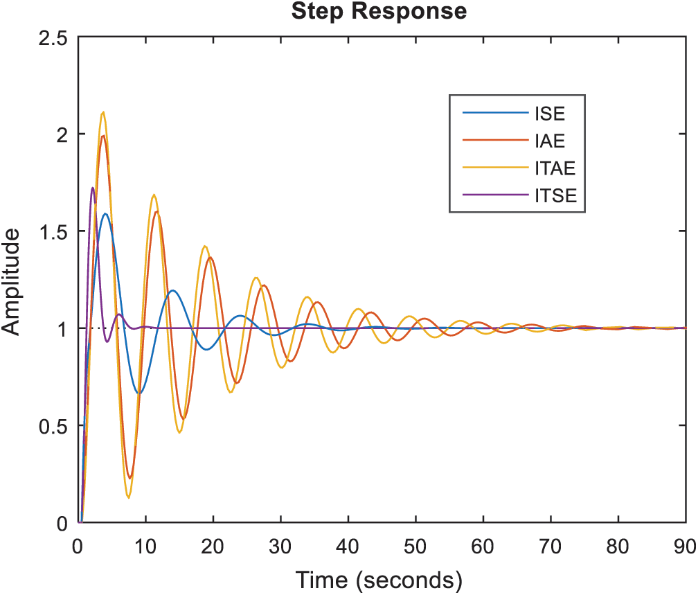
Figure 7: Step responses of closed-loop system

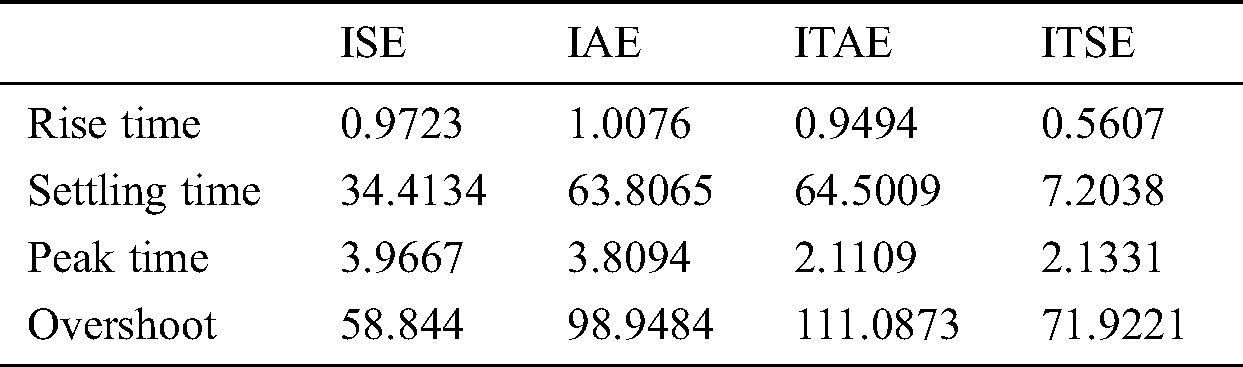
The time parameters and percentage overshoot values for unit step responses shown in Fig. 7 are given in Tab. 2.

Table 2: Time domain specifications

7  Conclusions

This study proposed the application of the Hermite-Biehler and GKT to defining the robust PID stability area for the control an of an uncertain and unstable second-order time-delay system. In the optimization process, the optimal system and optimal PID controller parameters are calculated by using the integral performance criterion based on the error.

Acknowledgement: The authors acknowledge the support of King Saud University, Saudi Arabia.

Funding Statement: The author(s) received no specific funding for this study.

Conflicts of Interest: The authors declare that they have no conflicts of interest to report regarding the present study.

References

1.  L. Dugard and E. I. Verriest. (1998). Stability and Control for Time Delay System. Berlin, Heidelberg: Springer-Verlag, pp. 5–10.

2.  C. Knospe. (2006). “PID control,” IEEE Control Systems Magazine, vol. 26, no. 1, pp. 30–31.

3.  G. J. Silva, A. Datta and S. P. Bhattacharyya. (2005). PID Controllers for Time Delay Systems. London, UK: Springer, pp. 12–22.

4.  R. Farkh, K. Laabidi and M. Ksouri. (2014). “Stabilizing sets of PI/PID controllers for unstable second order delay system,” International Journal of Automation and Computing, vol. 11, no. 2, pp. 210–222.

5.  B. R. Barmish, C. V. Holot, F. J. Kraus and R. Tempo. (1993). “Extreme points results for robust stabilization of interval plants with first order compensators,” IEEE Transaction on Automatic Control, vol. 38, no. 11, pp. 1734–1735.

6.  S. P. Bhattacharyya, H. Chapellat and L. H. Keel. (1995). Robust Control: The Parametric Approach. Upper Saddle River, NJ: Prentice-Hall, pp. 293–233.

7.  S. P. Bhattacharyya and H. Chapellat. (1989). “A generalization of Kharitonov’s theorem: Robust stability interval plants,” IEEE Transaction on Automatic Control, vol. 34, no. 3, pp. 306–311.

8.  K. Gu and V. Kharitonov. (1994). “Robust stability of time-delay systems,” IEEE Transaction on Automatic Control, vol. 39, no. 12, pp. 20–27.

This work is licensed under a Creative Commons Attribution 4.0 International License, which permits unrestricted use, distribution, and reproduction in any medium, provided the original work is properly cited.