DOI:10.32604/csse.2021.014189
| Computer Systems Science & Engineering DOI:10.32604/csse.2021.014189 | |
| Article |
Stock Price Forecasting: An Echo State Network Approach
1Hunan University of Finance and Economics, Changsha, China
2University Malaysia Sabah, Kota Kinabalu, Malaysia
3Yali High School International Department, Changsha, China
*Corresponding Author: Jingjing Lin. Email: 17573148817@163.com
Received: 04 September 2020; Accepted: 21 November 2020
Abstract: Forecasting stock prices using deep learning models suffers from problems such as low accuracy, slow convergence, and complex network structures. This study developed an echo state network (ESN) model to mitigate such problems. We compared our ESN with a long short-term memory (LSTM) network by forecasting the stock data of Kweichow Moutai, a leading enterprise in China’s liquor industry. By analyzing data for 120, 240, and 300 days, we generated forecast data for the next 40, 80, and 100 days, respectively, using both ESN and LSTM. In terms of accuracy, ESN had the unique advantage of capturing nonlinear data. Mean absolute error (MAE) was used to present the accuracy results. The MAEs of the data forecast by ESN were 0.024, 0.024, and 0.025, which were, respectively, 0.065, 0.007, and 0.009 less than those of LSTM. In terms of convergence, ESN has a reservoir state-space structure, which makes it perform faster than other models. Root-mean-square error (RMSE) was used to present the convergence time. In our experiment, the RMSEs of ESN were 0.22, 0.27, and 0.26, which were, respectively, 0.08, 0.01, and 0.12 less than those of LSTM. In terms of network structure, ESN consists only of input, reservoir, and output spaces, making it a much simpler model than the others. The proposed ESN was found to be an effective model that, compared to others, converges faster, forecasts more accurately, and builds time-series analyses more easily.
Keywords: Stock data forecast; echo state network; deep learning
In the era of big data, time-series data are present in domains such as stocks, traffic, electricity, and website traffic [1–3]. Research in this area, along with the mining of time-series data, has thus become valuable and challenging work [4,5]. Finance professionals devote a great deal of time and money to tapping the potential value of economic-, industry-, and enterprise-related data [6]. The forecasting and analysis of stock data have significant effects on countries, enterprises, and individuals. For countries, stock data forecasting can facilitate the macrocontrol of economic risks to promote financial reforms and stabilize economies [7,8]. Predictive data analysis can help enterprises raise funds. Further, using basic stock-trade data, investors can assess future market conditions to avoid risks and obtain higher returns [9].
The financial community has always focused on the difficult task of accurate stock trend forecasting [10,11]. In the era of big data, stock markets are influenced by the interactions of internal and external factors, including the effects of emergencies, and their complexity poses challenges for stock price research [12]. In the 1870s, most companies and researchers used traditional multiple linear statistical models to forecast stock trends, and with good results [13]. However, the amount of data has grown dramatically. Multiple linear models cannot capture big data—which have characteristics such as nonlinearity and spatiotemporal correlation—and have therefore fallen into disuse [14]. Neural networks and artificial intelligence subsequently appeared. With rapid increases in computing power, forecasting methods have moved in more intelligent directions [15,16]. For example, recurrent neural networks (RNN) have achieved high accuracy in stock forecasting [17,18]. However, neural networks have problems such as complex network structures, slow convergence, and high computational power consumption.
To deal with such challenges, this study used an echo state network (ESN) to forecast complex nonlinear stock data. Although ESN was introduced in 2001, its practical significance was not initially recognized, and it was only applied to pattern recognition. ESN’s advantages over RNNs and other neural networks include a simple structure, fast convergence, and the ability to capture nonlinearity [19].
The major contributions of this study can be summarized as follows:
• We used a lightweight ESN to solve problems in stock price forecasting related to complex network structures, slow convergence, and high computational costs.
• We conducted experiments using both ESN and long short-term memory (LSTM). We obtained error rates and convergence times and, analyzing the statistics, concluded that ESN performed better than traditional models.
• The experiments used in this study are universal and have great practical significance. The ESN structure is easily expanded and can be applied to other fields after modification.
Proposed by Herbert in 2001 [20], ESN is a type of RNN that uses reservoir calculation [21]. Initially, the study of ESN was only theoretical, and it was not until 2004 that Herbert applied it to wireless communication–related fields. Since then, researchers have worked to improve the model. Previous RNNs were unstable, had high computational complexity, and had slow convergence. ESN is simpler to calculate, has a shorter cycle, and is faster. ESN has thus made significant contributions to time-series forecasting and is widely applied in fields such as dynamic mode classification, robot control, object tracking, moving-target detection, and incident monitoring [22,23]. Fig. 1 shows the standard ESN structure. Consisting of an input, reservoir state, and output spaces [24], it can be described as a structural model with K input units, N reservoir processing elements, and L output units. Solid lines in the figure represent necessary connections, and dotted lines show possible or unnecessary connections. Dotted lines can also connect units in the input and output layers [25].

Figure 1: ESN structure
The input stock data vector  , output forecast value vector
  , and reservoir state space
  are expressed as vectors of size m, n, and p, respectively:


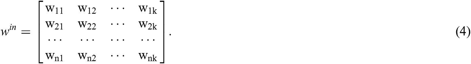
The reservoir is a sparse matrix whose degree is generally 0.01–0.1. The weight from the input layer to the reservoir, of order  , is
, is
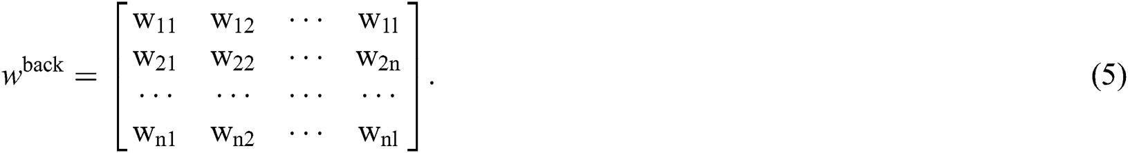
The feedback weight from the output layer to the reservoir is an  matrix:
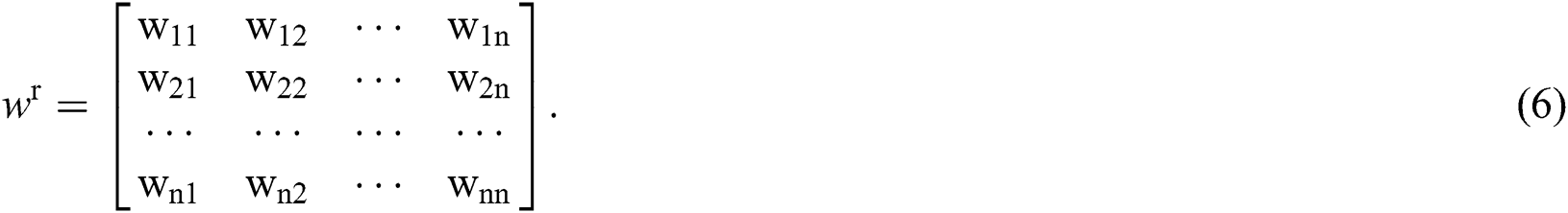
The reservoir is connected to the processing elements by an  matrix:
The reservoir is connected to the output layer units by an  matrix:

The connection between the output layer and the reservoir is unnecessary and is presented as a dotted line in Fig. 1.
The main difference between this model and that of a traditional neural network is that  ,
,  , and
, and  in ESN are initialized and set randomly when the network is established. Hence, little training is required, except the training of
  .
.
The reservoir will update its state when  is input at each moment. The state update equation is

and the state output equation is

where  is the state of the reservoir at the current moment,
  is the state at the previous moment,
 is the input at the current moment,
  is the activation function of the internal node of the reservoir, and
  is the activation function of the node of the output layer. The hyperbolic tangent function (
 ) is usually used for both
  and
and  .
.
The experiment had four steps: collect and clean data, set the experiment, forecast and analyze the data, and draw the experimental conclusion. Fig. 2 presents a flowchart of the experiment.
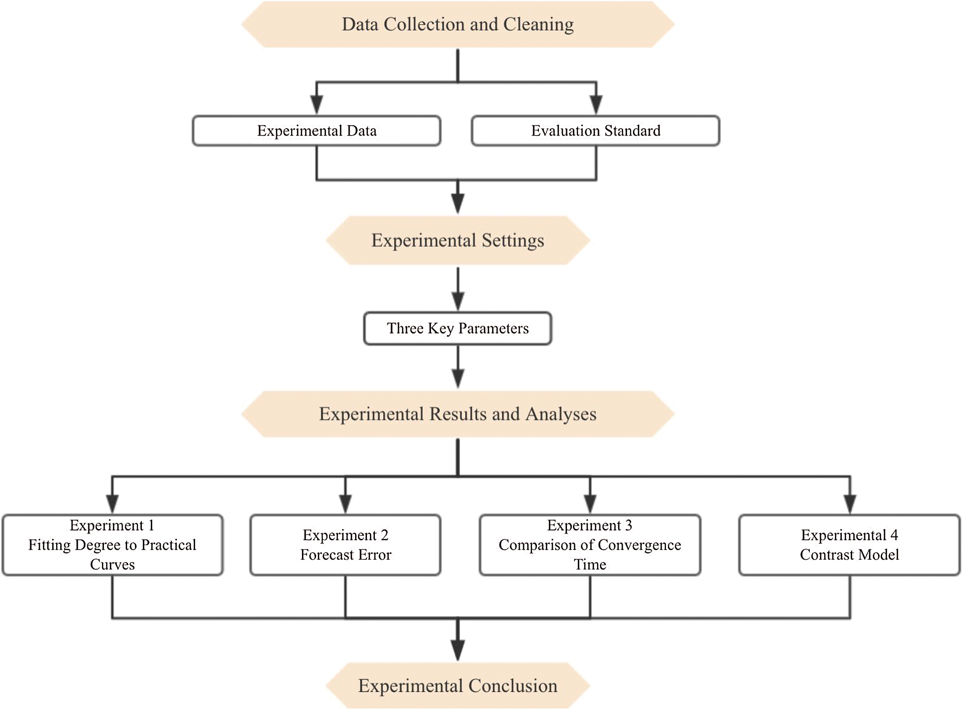
Figure 2: Flowchart of the experiment
3.1 Data Collection and Cleaning
We collected stock data for Kweichow Maotai (6000519. SH) on 360 trading days, from November 2, 2009, to April 26, 2011. Kweichow Maotai is a leading enterprise in China’s liquor industry, and no major equity changes occurred during the selected years. These stock data include volumes and opening, closing, highest, lowest, and adjusted closing prices. Data were sourced from Yahoo! Finance1.
Tab. 1 shows the closing prices in the 360-day transaction data for Kweichow Moutai (6000519. SH). Closing prices are the volume-weighted average prices of all trades (including the last trade) within the last minute of trading. Closing price could channel working funds in the next trading day while volumes, opening prices, highest prices, lowest prices, and adjusted prices cannot. Therefore, the closing price is very important for stock price forecasting and research.
Table 1: Stock data for Kweichow Moutai

We tested the closing prices in the 360-day transaction data for Kweichow Moutai. We compared the accuracy of different forecasting models and evaluated the performance of ESN based on the fitting degrees of forecast data and actual data, the mean absolute error (MAE) of forecast values and actual values, and the root-mean-square error (RMSE) of convergence time. MAE and RMSE are defined as


where  and
and  are the actual and forecast values, respectively, at time t, and N is the total number of forecast values, which equals 360 in the experiment.
The proposed ESN has three key parameters: spectral radius, size of reservoirs, and sparsity of reservoirs. If the spectral radius of the weighting  within the reservoir is less than 1, ESN will stay in an echo state. Reservoir size represents the number of neurons in the pool and is generally 300–500. Size is related to the number of samples, and it has a certain effect on network performance. A larger size means a more accurate stock forecast, but there will be an overfitting problem, while too small a size leads to underfitting. The sparsity of a reservoir represents the connections between its neurons, and not all neurons have connections. The more connections, the stronger the nonlinear approximation ability.
In this study, the reservoir was made up of 500 units. It scaled to a spectral radius of 0.999, and its sparsity was 0.02. The activation function for the reservoir processing elements was implemented as the tanh function, and the output function  was implemented as an identity function. We did not adopt the connection method denoted by the dotted line in Fig. 1.
The operating environment was Python 3.7.3 and Jupyter Notebook on Windows 10 Pro (64 bit). We used the pandas library to read closing stock prices and conduct experiments.
Conventional LSTM was modified to simplified LSTM by reducing training times. Simplified rather than conventional LSTM was used because stock price forecasts are in real time, and conventional LSTM cannot make valid calculations in a limited real-time range. We set up three experimental groups of 40-/80-/100-day data, which adopt ESN and simplified LSTM and one control group to compare the forecast data of ESN and LSTM. The three experimental groups used 120-day data to forecast the next 40 days’ closing prices, 240-day data for the next 80 days’ closing prices, and 300-day data for the next 100 days’ closing prices.
3.3 Experiment Results and Analyses
Experiment 1 was used to fit the forecast curves and practical curves. For both ESN and simplified LSTM, we used stock data for 120, 240, and 300 days as the training sample and data for 40, 80, and 100 days as the test sample.
The forecasting results were output by the two models over the three time-series data sets. We compared the forecasting results with the practical results through fitting graphs. Tab. 2 shows the results of the fitting tests for ESN and simplified LSTM. ESN fit well, and the overall effect of the model was good.

Figs. 3–5 show the fitting of the practical and forecasting results as output by the two forecasting models over three data sets. We used 120, 240, and 300 days of data to forecast stock closing prices in the next 40, 80, and 100 days.
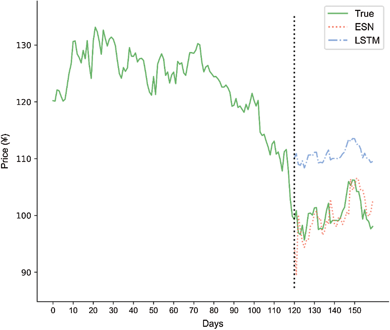
Figure 3: Comparison of ESN and LSTM price forecasts over 120 and 40 days
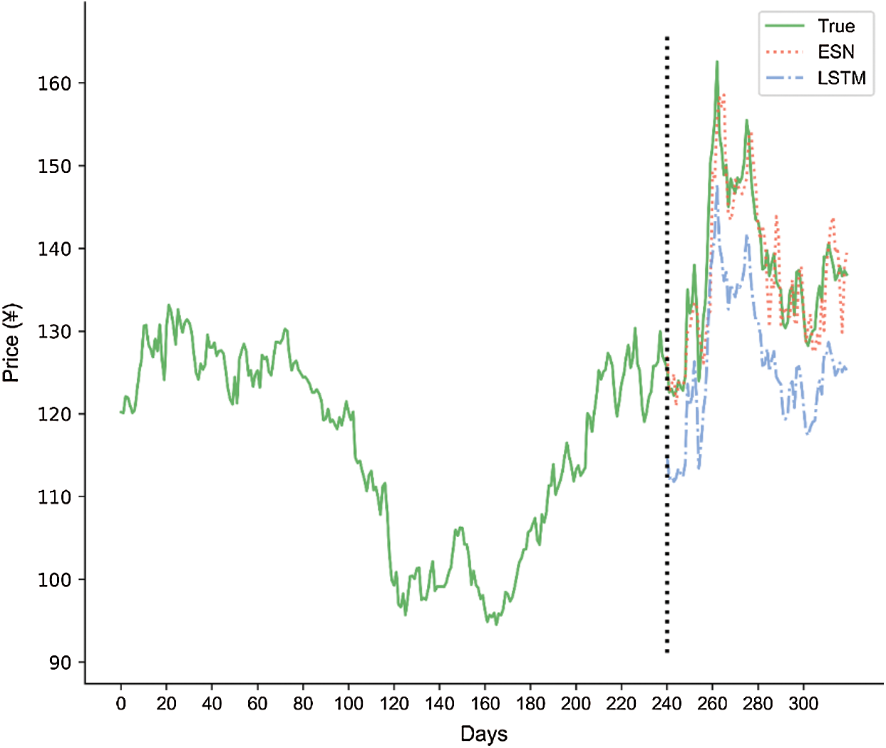
Figure 4: Comparison of ESN and LSTM price forecasts over 240 and 80 days
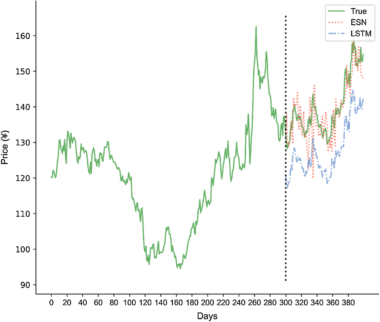
Figure 5: Comparison of ESN and LSTM price forecasts over 300 and 100 days
The fitting of the practical and forecasting results was better with ESN than with simplified LSTM. The forecasting results output by ESN fit the practical results well with lower curve amplitudes. These results indicate high forecasting accuracy. Meanwhile, because of poor data characteristics and parameter settings, the performance of simplified LSTM varied significantly. In conclusion, the proposed ESN exhibited advantages over simplified LSTM in time-series application.
We used the MAEs of the forecasting models on different data sets to evaluate forecasting accuracy. Tab. 3 shows the MAEs of different data sets output by the two forecasting models. A lower MAE indicates better performance. The MAE of data output by ESN was lower than that output by simplified LSTM. Thus, the result indicated that ESN performed well for forecasting.
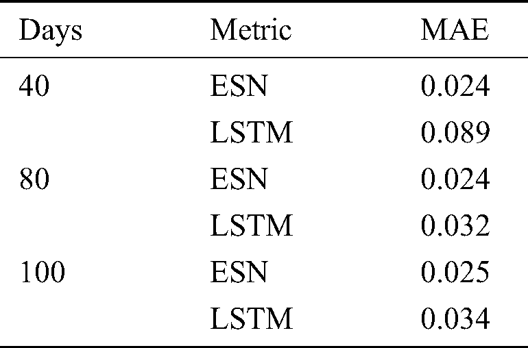
In forecasting, the error value trend of ESN gradually stabilized. In the three experimental groups, its error value was stable at around 0.024. Simplified LSTM’s performance was unstable. Its forecasting error sometimes fluctuated significantly while ESN showed relatively stable error values. ESN was consistent with actual stock fluctuation trends and could thus provide a reference for stock forecasting.
In summary, under the same conditions, the proposed ESN was more accurate than simplified LSTM. Analyzing the data and errors of the three experimental groups, ESN had fewer errors than simplified LSTM and was more consistent with the actual data. Therefore, ESN can forecast stock prices more quickly and accurately in the short term, reflecting market fluctuations.
Experiment 3 compared the convergence times of ESN and simplified LSTM with different data sets (Tab. 4). RMSE was used to present convergence time.

Tab. 4 shows that ESN had relatively few convergence times on three data sets. Compared to simplified LSTM, the convergence time advantage of ESN was not obvious for some data sets. However, the table also shows that, under the premise of ensuring high forecasting accuracy, ESN had relatively fewer convergence times than simplified LSTM.
Experiment 4 compared the closing price forecasts of simplified and conventional LSTM using 120 days’ data inputs.
As shown in Fig. 6, when simplified and conventional LSTM was used to forecast the closing price of the next 40 days, the more training time LSTM had, the more accurate the forecast. With an error value of 0.0078, the forecast of conventional LSTM fit the actual data well. However, in the experimental group, the error value between the forecast data of simplified LSTM and the actual data was 0.089. The gap between the error values of the different groups is obvious.

Figure 6: Comparison of simplified and conventional LSTM in price forecasts over 120 and 80 days
LSTM forecast data became more accurate as training times increased. This was because conventional LSTM can use the temporal backward-transfer algorithm to modify the weight according to previous errors. However, conventional LSTM took a lot of time. For ESN, while the training times are fixed, the updated state of the reservoir will not be as accurate as the error gradient of conventional LSTM.
ESN and LSTM were found to have advantages and disadvantages. ESN could quickly obtain forecasting results, which can help investors with short-term decision-making, but the error rate needs to be reduced. Conventional LSTM, meanwhile, reflects the characteristics of important events, which have long processing intervals and long delays in mid- and long-term stock forecasts. However, the problems of large volumes of data and time requirements remain unresolved. Therefore, compared to conventional LSTM, ESN has higher forecasting accuracy with a shorter processing time.
Stock price forecasting has time-series features. A neural network is a machine learning algorithm. ESN is a newer type of RNN. To obtain forecasting results using ESN, simply set the initial weights of the nodes and then input the nodes into the reservoir for recursive operation. Whether the output layer needs further training depends on the accuracy of the forecasting results. ESN requires less calculation because it does not need to repeatedly carry out training by calculating the gradient. However, many studies have shown that a stock forecast is a special nonlinear unstable event that is affected by both macro- and micro-factors. Thus, for the computing power of any single ESN model, it is difficult to include all of the complex influencing factors in the calculation and then obtain high forecasting accuracy. Therefore, in future work, we intend to combine conventional LSTM and ESN to leverage their respective advantages. ESN can improve convergence speed and better capture nonlinearity while conventional LSTM can forecast stock prices with little error. We believe a combined ESN and conventional LSTM model can be optimized to incorporate more factors that affect stock prices.
Funding Statement: This work was supported by the National Natural Science Foundation of China (No. 72073041); Open Foundation for the University Innovation Platform in Hunan Province (No. 18K103); 2011 Collaborative Innovation Center for Development and Utilization of Finance and Economics Big Data Property, Universities of Hunan Province, Open Project (Nos. 20181901CRP03, 20181901CRP04, 20181901CRP05); 2020 Hunan Provincial Higher Education Teaching Reform Research Project (Nos. HNJG-2020-1130, HNJG-2020-1124); and 2020 General Project of Hunan Social Science Fund (No. 20B16).
Conflicts of Interest: The authors declare that they have no conflicts of interest to report regarding the present study.
1. Y. Wu, Y. Liu, S. H. Ahmed, J. L. Peng and A. E. Ahmed. (2020). “Dominant data set selection algorithms for electricity consumption time-series data analysis based on affine transformation,” IEEE Internet of Things Journal, vol. 7, no. 5, pp. 4347–4360. [Google Scholar]
2. D. J. Bartholomew. (1971). “Time series analysis forecasting and control,” Journal of the Operational Research Society, vol. 22, no. 2, pp. 199–201. [Google Scholar]
3. Z. Y. Du. (2019). “Personal data security and supervision in the age of large data,” Intelligent Automation and Soft Computing, vol. 25, no. 4, pp. 847–853. [Google Scholar]
4. Y. Peng, Y. H. Liu and R. F. Zhang. (2019). “Modeling and analysis of stock price forecast based on lstm,” Computer Engineering and Applications, vol. 55, no. 11, pp. 209–212. [Google Scholar]
5. E. N. Qi and M. Deng. (2019). “R&D investment enhance the financial performance of company driven by big data computing and analysis,” Computer Systems Science and Engineering, vol. 34, no. 4, pp. 237–248. [Google Scholar]
6. F. M. Talarposhti, H. J. Sadaei, R. Enayatifar, F. G. Guimarães, M. Mahmud et al. (2016). , “Stock market forecasting by using a hybrid model of exponential fuzzy time-series,” International Journal of Approximate Reasoning, vol. 70, pp. 79–98. [Google Scholar]
7. M. P. O’Hare and F. J. Wen. (2018). “Research on hybrid model of garlic short-term price forecasting based on big data,” Computers, Materials & Continua, vol. 57, no. 2, pp. 283–296. [Google Scholar]
8. G. D. Zhao, Y. W. Zhang, Y. Q. Shi, H. Y. Lan and Q. Yang. (2019). “The application of BP neural networks to analysis the national vulnerability,” Computers, Materials & Continua, vol. 58, no. 2, pp. 421–436. [Google Scholar]
9. F. Xu, X. F. Zhang, Z. H. Xin and A. L. Yang. (2019). “Investigation on the Chinese text sentiment analysis based on convolutional neural networks in deep learning,” Computers, Materials & Continua, vol. 58, no. 3, pp. 697–709. [Google Scholar]
10. C. H. Zhang, J. Q. Yu and Y. Liu. (2019). “Spatial-temporal graph attention networks: A deep learning approach for traffic forecasting,” IEEE Access, vol. 7, pp. 166246–166256. [Google Scholar]
11. P. Gong and Y. Weng. (2016). “Value-at-risk forecasts by a spatiotemporal model in Chinese stock market,” Physica A: Statistical Mechanics and Its Applications, vol. 441, pp. 173–191. [Google Scholar]
12. J. L. Elman. (1990). “Finding structure in time,” Cognitive Science, vol. 14, no. 2, pp. 179–211. [Google Scholar]
13. M. I. Jordan, “Serial order: A parallel distributed processing approach,” Advances in Psychology, vol. 121, pp. 471–495, 1997. [Google Scholar]
14. S. Hochreiter and J. Schmidhuber. (1997). “Long short-term memory,” Neural Computation, vol. 9, no. 8, pp. 1735–1780. [Google Scholar]
15. Y. You, J. Hseu, C. Ying, J. Demmel, K. Keutzer et al. (2019). , “Large-batch training for LSTM and beyond,” Proceedings of the International Conference for High Performance Computing, Networking, Storage and Analysis, vol. 9, pp. 1–16. [Google Scholar]
16. G. B. Zhang, J. J. Xiong, Y. M. Huang, Y. Lu and L. Wang. (2018). “Delay-dependent stability of recurrent neural networks with time-varying delay,” Intelligent Automation and Soft Computing, vol. 24, no. 3, pp. 41–551. [Google Scholar]
17. A. G. Zhang, W. Zhu and J. Y. Li. (2018). “Spiking echo state convolutional neural network for robust time-series classification,” IEEE Access, vol. 7, pp. 4927–4935. [Google Scholar]
18. Q. L. Ma, E. H. Chen, Z. X. Lin, J. Y. Yan, Z. W. Yu et al. (2019). , “Convolutional multitimescale echo state network,” IEEE Transactions on Cybernetics, pp. 1–13. [Google Scholar]
19. J. Dan, W. Guo, W. Shi, B. Fang and T. Zhang. (2015). “PSO based deterministic ESN models for stock price forecasting,” Journal of Advanced Computational Intelligence and Intelligent Informatics, vol. 19, no. 2, pp. 312–318. [Google Scholar]
20. J. Herbert and H. Harald. (2004). “Harnessing nonlinearity: Predicting chaotic systems and saving energy in wireless communications,” Science, vol. 304, no. 5667, pp. 78–80. [Google Scholar]
21. J. Herbert. (2001). “The echo state approach to analyzing and training recurrent neural networks-with an erratum note,” in German National Research Center for Information Technology, Bonn, Germany, pp. 148. [Google Scholar]
22. X. J. Wang, Y. C. Jin and K. R. Hao. (2019). “Evolving local plasticity rules for synergistic learning in echo state networks,” IEEE Transactions on Neural Networks and Learning Systems, vol. 31, no. 4, pp. 1–12. [Google Scholar]
23. Y. Han, Y. W. Jing, K. Li and G. M. Dimirovski. (2019). “Network traffic prediction using variational mode decomposition and multi- reservoirs echo state network,” IEEE Access, vol. 7, pp. 138364–138377. [Google Scholar]
24. L. Wang, J. F. Qiao, C. L. Yang and X. X. Zhu. (2019). “Pruning algorithm for modular echo state network based on sensitivity analysis,” Acta Automatica Sinica, vol. 45, no. 6, pp. 1136–1145. [Google Scholar]
25. Y. Peng, M. Lei and J. Guo. (2011). “Clustered complex echo state networks for traffic forecasting with prior knowledge,” in IEEE Int. Instrumentation and Measurement Technology Conf., Binjiang, Hangzhou, China, vol. 78, pp. 1–5. [Google Scholar]
 | This work is licensed under a Creative Commons Attribution 4.0 International License, which permits unrestricted use, distribution, and reproduction in any medium, provided the original work is properly cited. |