DOI:10.32604/csse.2021.014894
| Computer Systems Science & Engineering DOI:10.32604/csse.2021.014894 | |
| Article |
Efficient Training of Multi-Layer Neural Networks to Achieve Faster Validation
Management Information Systems Department, College of Business, King Khalid University, Abha, Saudi Arabia
*Corresponding Author: Adel Saad Assiri. Email: adaseri@kku.edu.sa
Received: 25 October 2020; Accepted: 26 December 2020
Abstract: Artificial neural networks (ANNs) are one of the hottest topics in computer science and artificial intelligence due to their potential and advantages in analyzing real-world problems in various disciplines, including but not limited to physics, biology, chemistry, and engineering. However, ANNs lack several key characteristics of biological neural networks, such as sparsity, scale-freeness, and small-worldness. The concept of sparse and scale-free neural networks has been introduced to fill this gap. Network sparsity is implemented by removing weak weights between neurons during the learning process and replacing them with random weights. When the network is initialized, the neural network is fully connected, which means the number of weights is four times the number of neurons. In this study, considering that a biological neural network has some degree of initial sparsity, we design an ANN with a prescribed level of initial sparsity. The neural network is tested on handwritten digits, Arabic characters, CIFAR-10, and Reuters newswire topics. Simulations show that it is possible to reduce the number of weights by up to 50% without losing prediction accuracy. Moreover, in both cases, the testing time is dramatically reduced compared with fully connected ANNs.
Keywords: Sparsity; weak weights; multi-layer; neural network; NN; training with initial sparsity
The powerful tools of artificial intelligence are increasingly attractive for the analysis of real-life problems. Due to the proven efficiency of deep learning, artificial neural networks (ANNs) are the most frequently used strategy, with substantial applications and results in areas such as physics [1], engineering [2], and biology [3]. ANNs are usually composed of multiple layers of (artificial) neurons designed to replicate the functioning of biological neurons. In traditional ANN designs, all neurons are interconnected; that is, there exists a weight between all neurons, meaning that the number of weights is quadratic in the number of neurons. This leads to significant complexity of the learning process associated with a solution of an appropriate error minimization problem with respect to these weights. When the number of neurons is small, the complexity is feasible, but this can change as the number of neurons increases.
To resolve this issue, various fast and efficient learning strategies have been developed, including the scaled [4] and adaptive [5] conjugate gradient algorithms, adaptive learning rate method [6], sensitivity analysis [7], normalized perceptron-based methods [8], improved search methods [9], distributed Newton methods [10], and accelerated methods [11]. Alaba et al. [12] offered a comprehensive review of some recent advanced deep learning strategies. Pruning algorithms have also been shown to be quite effective in the analysis of various types of data. For a comparative study, see [13].
A novel method inspired by biological neural networks was proposed by Le Cun et al. [14] and developed by Mocanu et al. [15], in which weights between neurons are adaptively updated. Specifically, network initialization is accompanied by the creation of random weights. At each learning stage (epoch), weak weights, that is, those smaller than a prescribed threshold, are removed and new weights are created (see Fig. 1). Eventually, the training of the network is carried out only for strongly connected neurons, substantially reducing the complexity of the associated minimization problem. The pseudocode of the training algorithm, called the sparse evolutionary training (SET) algorithm, is shown in Algorithm 1.

Figure 1: Schematic representation of an ANN with sparse connectivity
Algorithm 1: Sparse evolutionary training pseudocode

A similar approach [16] suggested random dropouts of neurons together with their connections with other neurons. This “dropout” technique is often used to overcome overfitting problems. However, as shown below, it can also be used to train sparse ANNs.
This study aims to develop the idea of sparse connectivity by training networks with an initially reduced number of weights. Unlike Mocanu et al. [15], whose network was initially designed as fully connected and whose weights were adaptively updated during the learning process, we suggest the training with initial sparsity (TIS) method, which uses a reduced number of weights at network initialization and reduces weak weights during training. The simplest gradient descent algorithm is used for backpropagation (BP). A more advantageous learning algorithm can be developed using more advanced minimization techniques.
The rest of the paper is organized as follows. Section 3 presents the details and pseudocode of the algorithm. In Section 4, we apply TIS to the recognition of handwritten digits and Arabic characters and document the performance advantages of ANNs with reduced connectivity over the fully connected network. In Section 5, we compare TIS with similar methods. Conclusions and future research directions are discussed in Section 6.
Multi-layer neural networks have received significant attention and wide interest from scholars and scientists, as they are a powerful tool and efficient method in many fields, such as image processing [17], pattern recognition [18], natural language processing [19], VLSI design [20], and system diagnosis [21].
Yu et al. [22] developed a new ANN training technique in which neurons are computed neuron by neuron; they also implemented two different methods, namely, the Leveuberg–Marquardt (LM) and error backpropagation (EBP) methods. Schwenk et al. [23] presented a detailed survey on the best methods and practices of training a large ANN with more than 5.5 billion words. Adhikari et al. [24] developed a novel high-performance strategy for implementation in chip learning in multi-layer neural network hardware.
Recently, researchers used a metaheuristics algorithm in a multi-layer perceptron (MLP). Metaheuristics include the lightning search algorithm [25], ant lion optimization [26], the Salp swarm algorithm [27], moth-flame optimization [28], the whale optimization algorithm [29–32], and the crow search algorithm [33]. These algorithms have been successfully applied in training MLPs. MLPs can be employed in three different ways, which are each very efficient. First, an MLP can be used to obtain the weights of optimal connections. Second, it can be used to find the optimal architecture. Finally, it can be used to tune the arguments (parameters) of the algorithms.
TIS is a training algorithm for an ANN with reduced connectivity. By reducing the number of weights, we aim to improve the computational effectiveness of the testing (validation) process compared with a fully connected ANN. The reduction of weights should not substantially affect the accuracy. Thus, we seek faster validation without reducing accuracy and possibly improving it.
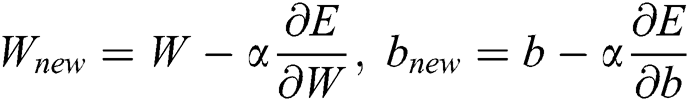
To illustrate, we construct a standard neural network with two hidden layers, where 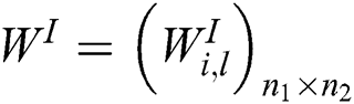 ,
, 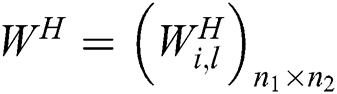 , and
, and 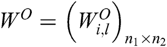 are matrices of the weights between the input and first hidden layer, first and second hidden layers, and second hidden layer and output layer, respectively;
  are bias vectors of the layers corresponding to their superscripts; and
 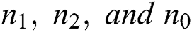 are the numbers of neurons in the corresponding layers.
The training process has two steps: forward and backward propagation. Forward propagation can be described as follows. Given an input vector 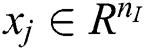 and a target vector
 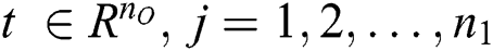 , consider the standard sigmoid function as the activation function:

whose responses for the first and second hidden layers will be


The real output 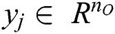 will then be evaluated as

In the BP stage, the standard quadratic error function is considered:

The gradient of  with respect to the weight matrices and bias vectors has the following components:


At the NN initialization step, random weights and biases are set. A prescribed level of initial sparsity is set by randomly removing the corresponding portions of the weights. Standard gradient descent is then used to update the remaining weights and biases according to the iterative procedure defined by
where  is a constant learning rate.
At each epoch from the first to the last, after updating all weights, the weak weights (those with absolute values close to zero) are removed and replaced by random weights. At the last epoch, weak weights are removed and not replaced. The pseudocode of this process is presented as Algorithm 2, and the corresponding flowchart is shown in Fig. 2.
Algorithm 2: Pseudocode for the sparse network process


Figure 2: Flowchart
As a simple application of the algorithm, we compare the performance of ANNs with reduced connectivity to that of fully connected ANNs. The algorithm was implemented in MATLAB and run on an Intel Core i7-4700MQ CPU @ 2.40 GHz (8 CPUs).
4.1 Handwritten Digits (MNIST Dataset)
First, we consider the publicly accessible MNIST dataset of handwritten digits, which contains 6·104 samples for learning and 104 for testing1 (see also [34] for a comparison of different machine learning algorithms for the MNIST dataset). Each sample was a 28 pixel × 28 pixel image. The data were in the  format, where
  is the input vector and
  is the perfect output guess. We set
  . Training was carried out with a fixed learning rate
  in 200 epochs with 5,000 learned samples per epoch.
By experimenting with different levels of initial sparsity, we observed that it is possible to achieve accuracy comparable to that of a corresponding fully connected NN even with substantially fewer weights. Tab. 1 shows that the NN with reduced number of weights has slightly better accuracy than the fully connected NN. Specifically, the accuracy of the NN with 50% initial sparsity was 0.65% higher.
Table 1: Accuracy of ANN for different levels of initial and total sparsity: MNIST dataset

Tab. 2 presents more quantitative information about the number of remaining weights, including the complexity of error minimization in the appropriate layer. Specifically, for a fully connected network, (1) must be minimized with respect to 25,544 weights; with 50% reduced weights, this number is 11,497.
Table 2: Number of remaining connections between layers for different levels of initial sparsity: MNIST dataset

However, as expected, higher levels of initial sparsity affect convergence. As Fig. 3 shows, when the level of initial sparsity is 50%, the error starts to decrease later than for a fully connected network. The difference occurs within the first 40 epochs.

Figure 3: Error propagation through epochs
The connectivity of visible neurons is plotted at different epochs of the training process in Fig. 4. A path between connectivity can be observed through the epochs, and it concentrates strong weights at the center of the sample. Weights near the sample boundary are too weak and therefore are removed. Such a picture should be expected, as the digits appear exactly in the domain of the samples where the visible neurons have the strongest weights.

Figure 4: Evolution of connectivity of visible neurons through epochs: handwritten digits
4.2 Handwritten Arabic Characters
The TIS algorithm was also applied to analyze the publicly accessible Arabic Handwritten Characters Dataset,2 which contains 13,440 samples for learning and 3,360 for testing. Each sample was a 32 pixel × 32 pixel image that was reshaped to a row vector of 1,024 elements. We set  ,
,  ,
,  , and
, and  . Training was carried out with a fixed learning rate of
  in 100 epochs with 5,000 learned samples per epoch.
In this case also, initially sparse NNs provided accuracies comparable to those of fully connected NNs even with substantially fewer weights. It can be seen from Tab. 3 that the indicators of accuracy of the NN with 5%, 15%, and 50% initial sparsity were higher than those of the corresponding fully connected NN by 0.6%, 1.02%, and 0.21%, respectively.
Table 3: Accuracy of ANN for different levels of initial and total sparsity: Arabic handwritten characters

The number of remaining weights for different levels of initial sparsity is presented in Tab. 4. It is worth noticing that compared with 325,500 weights in the case of a fully connected network, there are only 146,476 weights for the case of 50% initial sparsity.
Table 4: Number of remaining connections between layers for different levels of initial sparsity: Arabic handwritten characters

The connectivity of visible neurons at different epochs of the training process is plotted for this case in Fig. 5. Through epochs, strong weights were concentrated around the domain where Arabic letters appear. Weaker weights were concentrated near sample boundaries and therefore were removed.

Figure 5: Evolution of connectivity of visible neurons through epochs: handwritten Arabic characters
A straightforward consequence of reduced weights is the dramatic reduction of the time spent testing the test samples (see Fig. 6).
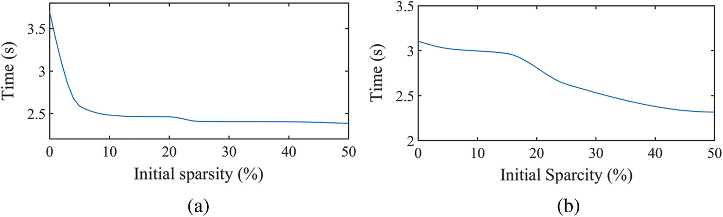
Figure 6: Dependence of testing time on initial sparsity level: (a) MNIST, with 104 testing samples; (b) Arabic handwritten characters, with 3,360 testing samples
It is easy to see that our algorithm does not depend on the choice of the BP algorithm.
4.3 Comparing Validation Accuracies of Various Training Algorithms
As mentioned above, we chose the simplest training algorithm for BP, namely, gradient descent. We compare the validation time versus initial sparsity with some other BP algorithms. These are the well-known conjugate gradient, quasi-Newton, and Levenberg–Marquardt algorithms (see Tab. 5).
Table 5: Accuracies of different backpropagation algorithms with 50% initial sparsity

5 Comparison with Existing Methods
We compare TIS with the SET [15] and DO [16] methods on three datasets: MNIST, CIFAR-10,3 and Keras Dataset Reuters newswire topics (RNT). The CIFAR-10 dataset consists of 60,000 32 pixel × 32 pixel color images in 10 classes with 6,000 images per class. There are 50,000 training samples and 10,000 test samples. RNT consists of 11,228 newswires from Reuters, labeled over 46 topics. Each wire is encoded as a sequence of word indices. We used the following BP algorithms: conjugate gradient, gradient descent, quasi-Newton, and Levenberg–Marquardt. Comparative analysis indicates that TIS has advantages over SET and DO for all BP algorithms. Therefore, in the interest of brevity, we carry out the comparison analysis only for the gradient descent BP algorithm.
Open-source implementations are freely available for both SET4 and DO.5 We use these implementations to benchmark the performance of TIS against the other two methods.
We compare the performance of SET, DO, and TIS on the MNIST dataset considered in Section 3.1. For TIS with 50% initial sparsity (Fig. 7b), the accuracy of TIS increases much faster. It is also evident that TIS ensures a faster convergence rate. Fig. 7b shows that TIS with 50% initial sparsity has the highest convergence acceleration among the tested methods.

Figure 7: Benchmarking TIS, SET, and DO on the MNIST dataset: (a) accuracy plot for TIS with 25% initial sparsity, DO with 7.5% rate, and SET with 25% sparsity; (b) accuracy plot for TIS with 50% initial sparsity, DO with 5% rate, and SET with 50% sparsity; (c) convergence plot for TIS with 25% initial sparsity, DO with 7.5% rate, and SET with 25% sparsity; (d) convergence plot for TIS with 50% initial sparsity, DO with 5% rate, and SET with 25% sparsity
We compare the performance of TIS, SET, and DO on the CIFAR-10 dataset. Fig. 8 demonstrates that TIS has an advantage over SET and DO in both accuracy and convergence.

Figure 8: Benchmarking TIS, SET, and DO on the CIFAR-10 dataset: (a) accuracy plot for TIS with 25% initial sparsity, DO with 10% rate, and SET with 25% sparsity; (b) accuracy plot for TIS with 50% initial sparsity, DO with 7.5% rate, and SET with 50% sparsity; (c) convergence plot for TIS with 25% initial sparsity, DO with 10% rate, and SET with 25% sparsity; (d) convergence plot for TIS with 50% initial sparsity, DO with 7.55% rate, and SET with 25% sparsity
We compare the performance of SET, DO, and TIS on the RNT dataset. For TIS with 50% initial sparsity (Fig. 9b), the accuracy of TIS increases much more quickly. It is also evident that TIS ensures a faster convergence rate. Fig. 9b shows that TIS with 50% initial sparsity has the highest convergence acceleration among the tested methods.

Figure 9: Benchmarking TIS, SET, and DO on RNT dataset: (a) accuracy plot for TIS with 25% initial sparsity, DO with 15% rate, and SET with 25% sparsity; (b) accuracy plot for TIS with 50% initial sparsity, DO with 10% rate, and SET with 50% sparsity; (c) convergence plot for TIS with 25% initial sparsity, DO with 15% rate, and SET with 25% sparsity; (d) convergence plot for TIS with 50% initial sparsity, DO with 10% rate, and SET with 50% sparsity
As artificial neurons are designed to mimic the functioning of biological neurons, it is natural to expect that artificial neural networks should possess the key features of biological neural networks, which would lead to efficient learning. Features reported to have a significant impact on learning efficiency include sparsity [35,36], scale-freeness [37], and small-worldness [38]. Mocanu et al. [15] designed a sparse and scale-free ANN, which was shown to substantially enhance learning efficiency. In our method, at the initial step, the ANN is assumed to be fully connected; weights with small absolute values are removed; and new random weights are added (see Algorithm 1).
In this study, we introduced the concept of initial sparsity, that is, the ANN is assumed to be sparse at the initial step, with the possibility to prescribe the level of initial sparsity. At each training epoch, weights that are close to zero in absolute value are removed, and random weights are added (see Algorithm 1). The test network has two hidden layers. Comparative analysis shows that networks with initial sparsity of up to 50% exhibit better accuracy than the initial fully connected network. Moreover, it is observed that after training is finished, the testing time dramatically decreases with the increase of the initial sparsity level. It is also observed that convergence of the error is slower for initial sparsity levels greater than 40% (compared with an initially fully connected network). Comparative analysis shows that the gradient descent, quasi-Newton, and Levenberg–Marquardt BP algorithms increase the accuracy of validation compared with gradient descent BP (with 50% initial sparsity).
The proposed method was also compared with other similar methods, namely, SET and DO. An analysis was carried out on the MNIST, CIFAR-10, and RNT datasets. The analysis showed that TIS outperforms both SET and DO in accuracy and convergence rate. These observations apply to the four tested BP algorithms: conjugate gradient, gradient descent, quasi-Newton, and Levenberg–Marquardt.
These observations motivate us to improve the general algorithm, which will be a focus of future work. In this study, we used gradient descent, one of the simplest BP methods, for error minimization. A priority of future work will be to implement the developed algorithm with more advanced minimization strategies, such as the modified conjugate gradient descent and distributed Newton methods, combined with a more efficient line search strategy. We also intend to test the algorithm on some variants of convolutional neural networks. Another challenging problem is the optimal choice of the level of initial sparsity in the context of the network structure and the particular dataset.
Acknowledgement: I express my gratitude to King Khalid University, Saudi Arabia, for administrative and technical support.
Funding Statement: The author received no specific funding for this study.
Conflicts of Interest: The author declares no conflicts of interest regarding the present study.
1. R. Iten, T. Metger, H. Wilming, L. del Rio and R. Renner. (2018). “Discovering physical concepts with neural networks,” arXiv:1807.10300. [Google Scholar]
2. A. Y. Alanis, N. Arana-Daniel and C. López-Franco. (2019). Artificial Neural Networks for Engineering Applications. Cambridge, MA, USA: Academic Press. [Google Scholar]
3. H. M. Cartwright. (2008). “Artificial neural networks in biology and chemistry—the evolution of a new analytical tool,” in Artificial Neural Networks: Methods and Applications. Totowa, NJ, USA: Humana Press, pp. 1–13. [Google Scholar]
4. M. F. Møller. (1993). “A scaled conjugate gradient algorithm for fast supervised learning,” Neural Networks, vol. 6, no. 4, pp. 525–533. [Google Scholar]
5. H. Adeli and S. L. Hung. (1994). “An adaptive conjugate gradient learning algorithm for efficient training of neural networks,” Applied Mathematics and Computation, vol. 62, no. 1, pp. 81–102. [Google Scholar]
6. H. B. Kim, S. H. Jung, T. G. Kim and K. H. Park. (1996). “Fast learning method for back-propagation neural network by evolutionary adaptation of learning rates,” Neurocomputing, vol. 11, no. 1, pp. 101–106. [Google Scholar]
7. E. Castillo, B. Guijarro-Berdiñas, O. Fontenla-Romero and A. Alonso-Betanzos. (2006). “A very fast learning method for neural networks based on sensitivity analysis,” Journal of Machine Learning Research, vol. 7, pp. 1159–1182. [Google Scholar]
8. X. Xie, H. Qu, G. Liu and M. Zhang. (2017). “Efficient training of supervised spiking neural networks via the normalized perceptron based learning rule,” Neurocomputing, vol. 241, pp. 152–163. [Google Scholar]
9. J. Wang, B. Zhang, Z. Sun, W. Hao and Q. Sun. (2018). “A novel conjugate gradient method with generalized Armijo search for efficient training of feedforward neural networks,” Neurocomputing, vol. 275, pp. 308–316. [Google Scholar]
10. C. C. Wang, K. L. Tan, C. T. Chen, Y. H. Lin, S. S. Keerthi et al. (2018). , “Distributed newton methods for deep neural networks,” Neural Computation, vol. 30, no. 6, pp. 1673–1724. [Google Scholar]
11. P. Skryjomski, B. Krawczyk and A. Cano. (2019). “Speeding up k-Nearest Neighbors classifier for large-scale multi-label learning on GPUs,” Neurocomputing, vol. 354, pp. 10–19. [Google Scholar]
12. P. A. Alaba, S. I. Popoola, L. Olatomiwa, M. B. Akanle, O. S. Ohunakin et al. (2019). , “Towards a more efficient and cost-sensitive extreme learning machine: A state-of-the-art review of recent trend,” Neurocomputing, vol. 350, pp. 70–90. [Google Scholar]
13. M. Augasta and T. Kathirvalavakumar. (2013). “Pruning algorithms of neural networks—a comparative study,” Central European Journal of Computer Science, vol. 3, no. 3, pp. 105–115. [Google Scholar]
14. Y. Le Cun, J. S. Denker and S. A. Solla. (1989). “Optimal brain damage,” in Proc. NIPS'89, Denver, CO, USA, pp. 598–605. [Google Scholar]
15. D. C. Mocanu, E. Mocanu, P. Stone, P. H. Nguyen, M. Gibescu et al. (2018). , “Scalable training of artificial neural networks with adaptive sparse connectivity inspired by network science,” Nature Communications, vol. 9, pp. 2383. [Google Scholar]
16. N. Srivastava, G. Hinton, A. Krizhevsky, I. Sutskever and R. Salakhutdinov. (2014). “Dropout: A simple way to prevent neural networks from overfitting,” Journal of Machine Learning Research, vol. 15, no. 1, pp. 1929–1958. [Google Scholar]
17. O. A. Ahmed and M. M. Fahmy. (1997). “Application of multi-layer neural networks to image compression,” in 1997 IEEE International Sym. on Circuits and Systems (ISCASIEEE, vol. 2, pp. 1273–1276. [Google Scholar]
18. G. Daqi and W. Shouyi. (1998). “An optimization method for the topological structures of feed-forward multi-layer neural networks,” Pattern Recognition, vol. 31, no. 9, pp. 1337–1342. [Google Scholar]
19. M. Guan, S. Cho, R. Petro, W. Zhang, B. Pasche et al. (2019). , “Natural language processing and recurrent network models for identifying genomic mutation-associated cancer treatment change from patient progress notes,” JAMIA Open, vol. 2, no. 1, pp. 139–149. [Google Scholar]
20. K. Cameron and A. Murray. (2008). “Minimizing the effect of process mismatch in a neuromorphic system using spike-timing-dependent adaptation,” IEEE Transactions on Neural Networks, vol. 19, no. 5, pp. 899–913. [Google Scholar]
21. J. F. Martins, V. Ferno Pires and A. J. Pires. (2007). “Unsupervised neural-network-based algorithm for an on-line diagnosis of three-phase induction motor stator fault,” IEEE Transactions on Industrial Electronics, vol. 54, no. 1, pp. 259–264. [Google Scholar]
22. H. Yu and B. M. Wilamowski. (2009). “Efficient and reliable training of neural networks,” in 2009 2nd Conf. on Human System Interactions, IEEE, pp. 109–115. [Google Scholar]
23. H. Schwenk, F. Bougares and L. Barrault. (2014). “Efficient training strategies for deep neural network language models,” in NIPS workshop on Deep Learning and Representation Learning, Montreal, Canada. [Google Scholar]
24. S. P. Adhikari, C. Yang, K. Slot, M. Strzelecki and H. Kim. (2018). “Hybrid no-propagation learning for multilayer neural networks,” Neurocomputing, vol. 321, pp. 28–35. [Google Scholar]
25. L. Abualigah, M. Abd Elaziz, A. G. Hussien, B. Alsalibi, S. M. J. Jalali et al. (2020). , “Lightning search algorithm: A comprehensive survey,” Applied Intelligence, pp. 1–24. [Google Scholar]
26. A. S. Assiri, A. G. Hussien and M. Amin. (2020). “Ant Lion Optimization: Variants, hybrids, and applications,” IEEE Access, vol. 8, pp. 77746–77764. [Google Scholar]
27. A. G. Hussien, A. E. Hassanien and E. H. Houssein. (2017). “Swarming behaviour of salps algorithm for predicting chemical compound activities,” in 2017 Eighth Int. Conf. on Intelligent Computing and Information Systems (ICICISIEEE, pp. 315–320. [Google Scholar]
28. A. G. Hussien, M. Amin and M. Abd El Aziz. (2020). “A comprehensive review of moth-flame optimisation: Variants, hybrids, and applications,” Journal of Experimental & Theoretical Artificial Intelligence, vol. 32, no. 4, pp. 1–21. [Google Scholar]
29. A. G. Hussien, D. Oliva, E. H. Houssein, A. A. Juan and X. Yu. (2020). “Binary whale optimization algorithm for dimensionality reduction,” Mathematics, vol. 8, no. 10, pp. 1821. [Google Scholar]
30. A. G. Hussien, A. E. Hassanien, E. H. Houssein, M. Amin and A. T. Azar. (2020). “New binary whale optimization algorithm for discrete optimization problems,” Engineering Optimization, vol. 52, no. 6, pp. 945–959. [Google Scholar]
31. A. G. Hussien, A. E. Hassanien, E. H. Houssein, S. Bhattacharyya and M. Amin. (2019). “S-shaped binary whale optimization algorithm for feature selection,” in Recent trends in signal and image processing. Singapore: Springer, pp. 79–87. [Google Scholar]
32. A. G. Hussien, E. H. Houssein and A. E. Hassanien. (2017). “A binary whale optimization algorithm with hyperbolic tangent fitness function for feature selection,” in 2017 Eighth Int. Conf. on Intelligent Computing and Information Systems (ICICISIEEE, pp. 166–172. [Google Scholar]
33. A. G. Hussien, M. Amin, M. Wang, G. Liang, A. Alsanad et al. (2020). , “Crow search algorithm: Theory, recent advances, and applications,” IEEE Access, vol. 8, pp. 173548–173565. [Google Scholar]
34. H. Xiao, K. Rasul and R. Vollgraf. (2017). “Fashion-mnist: A novel image dataset for benchmarking machine learning algorithms,” arXiv:1708.07747. [Google Scholar]
35. S. H. Strogatz. (2001). “Exploring complex networks,” Nature, vol. 410, no. 6825, pp. 268–276. [Google Scholar]
36. L. Pessoa. (2014). “Understanding brain networks and brain organization,” Physics of Life Reviews, vol. 11, no. 3, pp. 400–435. [Google Scholar]
37. A. L. Barabási and R. Albert. (1999). “Emergence of scaling in random networks,” Science, vol. 286, no. 5439, pp. 509–512. [Google Scholar]
38. E. Bullmore and O. Sporns. (2009). “Complex brain networks: Graph theoretical analysis of structural and functional systems,” Nature Reviews: Neuroscience, vol. 10, no. 3, pp. 186–198. [Google Scholar]
 | This work is licensed under a Creative Commons Attribution 4.0 International License, which permits unrestricted use, distribution, and reproduction in any medium, provided the original work is properly cited. |