Computer Systems Science & Engineering DOI:10.32604/csse.2021.015146
Article

A New Generalized Weibull Model: Classical and Bayesian Estimation

Mi Zichuan1, Saddam Hussain1, Zubair Ahmad2,*, Omid Kharazmi3 and Zahra Almaspoor2

1School of Statistics, Shanxi University of Finance and Economics, Taiyuan, China
2Department of Statistics, Yazd University, Yazd, Iran
3Department of Statistics, Faculty of Sciences, Vali-e-Asr University of Rafsanjan, Rafsanjan, Iran
*Corresponding Author: Zubair Ahmad. Email: z.ferry21@gmail.com
Received: 08 November 2020; Accepted: 27 December 2020

Abstract: Statistical distributions play a prominent role in applied sciences, particularly in biomedical sciences. The medical data sets are generally skewed to the right, and skewed distributions can be used quite effectively to model such kind of data sets. In the present study, therefore, we propose a new family of distributions suitable for modeling right-skewed medical data sets. The proposed family may be called a new generalized-X family. A special sub-model of the proposed family called a new generalized-Weibull distribution is discussed in detail. The maximum likelihood estimators of the model parameters are obtained. A brief Monte Carlo simulation study is conducted to evaluate the performance of these estimators. Finally, the proposed model is applied to the remission times of the stomach cancer patient’s data. The comparison of the goodness of fit results of the proposed model is made with the other competing models such as Weibull, Kumaraswamy Weibull, and exponentiated Weibull distributions. Certain analytical measures such as Akaike information criterion, Bayesian information criterion, Anderson Darling statistic, and Kolmogorov–Smirnov test statistic are considered to show which distribution provides the best fit to data. Based on these measures, it is showed that the proposed distribution is a reasonable candidate for modeling data in medical sciences and other related fields.

Keywords: Weibull distribution; stomach cancer; hazard function; statistical modeling; akaike information criterion

1  Introduction

In medical situations, for example, neck cancer, bladder cancer, stomach cancer, and breast cancer, etc., the hazard rate is shown to have unimodal or modified unimodal shape. The hazard rate for neck, bladder, and breast cancer recurrence after surgical removal has been observed to have unimodal shape. In the very initial phase, the hazard rate for cancer recurrence begins with a low level and then increases gradually after a finite period of time after the surgical removal until reaching a peak before decreasing. Another example of the unimodal shape is the hazard of infection with some new viruses, where it increases in the early stages from a low level till it reaches a peak and then decreases; see Liao et al. [1].

The parametric methods such as the exponential, Rayleigh, Weibull, lognormal and gamma distributions have been extensively used in fitting bio-medical data; see Zhu et al. [2]. The researchers in medical sciences have shown a great interest in studying the survival of patients, particularly, patients with cancer [3]. An appropriate parametric model is always of interest in survival analysis, as it provides a concise description of the characteristics of failure times as well as hazard function that may not be available with non-parametric methods [4]. The parametric Weibull is a more flexible distribution than the Cox semi-parametric model, since; the associated hazard rate is not constant over time.

No doubt, that the parametric models stated above are used frequently in survival analysis. However, unfortunately, still, these models are subject to some sort of deficiencies; see Ahmad et al. [5]. For more information, we refer to [6–11]. The next section offers a brief description of the deficiencies associated with the former parametric models.

2  Problems Associated with the Former Models

As we mentioned earlier, that the exponential, Rayleigh, and Weibull are the most frequently used distributions among the parametric models. These distributions, however, are not flexible enough to counter complex forms of the data. For example, the exponential distribution is capable of modeling data with a constant hazard rate function (hrf), only. The hrf of the exponential distribution is given by

h(x;γ)=γ,x>0,γ>0, (1)

which is constant.

On the other hand, the Rayleigh distribution offers data modeling with only increasing hrf. Let X∼Ray(γ), then hrf of the Rayleigh distribution is given by

h(x;γ)=2γx,x>0,γ>0, (2)

From Eq. (2), we can see that the Rayleigh distribution is capable of modeling real-life data with increasing hrf, only.

Among the parametric models, the Weibull distribution is one of the most commonly used family for modeling such data offering the characteristics of both the exponential and Rayleigh distributions is given by

h(x;α,γ)=αγxα−1,x>0,α>0,γ>. (3)

From Eq. (3), we can easily observe that the Weibull distribution is capable of modeling lifetime data with monotonically increasing, constant, and decreasing hazard functions, depending on the shape parameter α . Unfortunately, the Weibull distribution is not capable of modeling data with non-monotonic (unimodal, modified unimodal and bathtub shaped) hrf. For γ = 1 and different values of α , plots for the hazard function of the Weibull distribution are presented in Fig. 1.

Figure 1: Plots of hazard rate function of the Weibull distribution

Among the available literature, the frequently used Kaplan–Meier product-limit estimator is one of the flexible methods to model survival data. But, as observed in Miller [12], this method is often inefficient. Other semi-parameter approaches such as proportional hazards modeling need many assumptions that may not feasible; see Cox et al. [13]. Meanwhile, a number of parametric approaches have been introduced to incorporate a wide variety of patterns in survival data. Some proposed parametric models have incorporated a shape parameter into the classic Weibull distribution to account for additional possible hazard shapes. Among them, one such method is proposed by Kalbfleisch et al. [14], this model may be impractical in the presence of censored data, as it often requires the evaluation of an incomplete gamma integral or beta ratio. In the premises of the above, the medical researchers are always in search of introducing new distributions capable of modeling lifetime data with unimodal hazard function. In this regard, a serious attempt has been made and still growing rapidly; see Ahmad et al. [15].

Under these premises, we are motivated to propose new families of distributions. Therefore, in this article, an attempt has been made to propose a new family of distributions to provide the best fit to data in medical sciences and other related fields.

The paper is outlined as follows: the proposed method is presented in Section 3. In Section 4, we define a special sub-model of the proposed family. The maximum likelihood estimation of the model parameters is addressed in Section 5. The source and nature of the data are discussed in Section 6. Model selection criteria are presented in Section 7. In Section 8, we provide a real-life application from medical sciences to illustrate the importance of the new family. Section 9 is devoted to the Bayesian analysis of the data. Finally, some concluding remarks are presented in Section 10.

3  Development of the Proposed Method

Let v(t) be the probability density function (pdf) of a random variable, say T , where T∈[m,n] for −∞≤m∠n∠∞, and let W[F(x)] be a function of cumulative distribution function (cdf) of a random variable, say X, satisfying the conditions given below:

•     W[F(x)]∈[m,n] ,

•     W[F(x)] is differentiable and monotonically increasing, and

•     W[F(x)]→m as x→−∞ and W[F(x)]→n as x→∞ .

The cdf of the T-X family of distributions; see Alzaatreh et al. [16] is defined by

G(x)=∫mW[F(x)]v(t)dt,x∈R (4)

where, W[F(x)] satisfies the conditions stated above. The pdf corresponding to Eq. (4) is

g(x)={∂∂xW[F(x)]}v{W[F(x)]},x∈R

Using the T-X family idea, several new classes of distributions have been introduced in the literature. Now, we introduce the proposed family. Let T∼exp⁡(1), then its cdf is given by

V(t)=1−e−t,t≥0 (5)

The density function corresponding to Eq. (5) is

v(t)=e−t,t>0 (6)

If v(t) follows Eq. (6) and setting W[F(x)]=log⁡(log⁡(1+θ−θF(x;ξ)θlog⁡(1+θ) in Eq. (4), we define the cdf of the NG-X family by

G(x)=1−(log⁡(1+θ−θF(x;ξ)θlog⁡(1+θ),x∈R. (7)

The density function corresponding to Eq. (7) is

g(x)=θ2f(x;ξ)F(x;ξ)θ−1log⁡(1+θ)(1+θ−θF(x;ξ)θ),x∈R. (8)

The key motivations for using the NG-X distributions in practice are the following:

•   A very simple and convenient method to modify the existing distributions.

•   To improve the characteristics and flexibility of the existing distributions.

•   To introduce the extended version of the baseline distribution having closed form of distribution function.

•   To provide the best fit to data in the medical sciences and other related fields.

•   Another most important motivation of the proposed approach is to introduce new distributions by adding only one additional parameter rather than adding two or more parameters.

4  Sub-Model Description

In this section, we introduce a special sub-model of the proposed family, called a new generalized Weibull (NG-W) distribution. Let F(x;ξ) be the cdf of the Weibull distribution given by F(x;ξ)=1−e−γxα, x≥0, α,γ>0, where ξ=(α,λ) . Then, the cdf of the NG-W has the following expression

G(x;θ,ξ)=1−(log⁡(1+θ−θ(1−e−γxα)θ)log⁡(1+θ)),x≥0,α,γ,θ>0. (9)

The pdf and hrf of the NG-W model are given, respectively, by

g(x;θ,ξ)=αθ2γxα−1e−γxα(1−e−γxα)θ−1log⁡(1+θ)(1+θ−θ((1−e−γxα)θ),x>0, (10)

and

h(x;θ,ξ)=αθ2γxα−1e−γxα(1−e−γxα)θ−1log⁡(1+θ−θ((1−e−γxα)θ)(1+θ−θ((1−e−γxα)θ),x>0.

For different values of the model parameters, plots of the density function of the NG-W distribution are sketched in Fig. 2.

Figure 2: Different plots for the density function of the NG-W distribution

The plots for the hrf of the NG-W distribution are presented in Figs. 3 and 4.

Figure 3: Increasing and decreasing hazard functions of the NG-W distribution

Figure 4: Unimodal hrf of the NG-W distribution

5  Maximum Likelihood Estimation

Here, we obtain the maximum likelihood estimators (MLEs) of the model parameters of the NG - W distribution. Let x1,x2…,xn be the observations from pdf given in Eq. (10) with parameters α,θ and γ . Then, the log-likelihood function corresponding to Eq. (11) is given by

L(xi,α,θ,γ)=nlog⁡α+2nlog⁡θ+nlog⁡γ+(α−1)−nlog⁡(log⁡(1+θ))−∑i=1nlog⁡(1+θ−θ(1−e−γxiα)). (11)

The log-likelihood function can be maximized either directly or by solving the nonlinear likelihood function obtained by differentiating Eq. (11). We used the goodness of fit function in R with “Nelder-Mead” algorithm to obtain the MLEs. The first order partial derivatives of Eq. (11) with respect to the parameters are given, respectively, by

∂∂αL(xi,α,θ,γ)=nα+∑i=1nlog⁡xi+(θ−1)γ∑i=1nlog⁡(xi)xiαe−γxiα1−e−γxiα+θγ∑i=1n(log⁡xi)xiαe−γxiα(1+θ−θ(1−e−γxiα)), (12)

∂∂θL(xi,α,θ,γ)=2nθ+∑i=1nlog⁡(1−e−γxiα)−n(log⁡(1+θ))(1+θ)−∑i=1n(e−γxa(1+θ−θ(1−e−γxiα)), (13)

and

∂∂γL(xi,α,θ,γ)=nγ+(θ−1)∑i=1nxiαe−γxiα(1−e−γxiα)+∑i=1nθxiαe−γxiα(1+θ−θ(1−e−γxiα)). (14)

Setting ∂∂αL(xi,α,θ,γ) , ∂∂θL(xi,α,θ,γ) and ∂∂γL(xi,α,θ,γ) equal to zero and solving numerically these expressions simultaneously yields the MLEs of (α,θ,γ) . From Eqs. (12)–(14), it is clear that these expressions are not in closed form. Therefore, computer software with the iterative methods used such as the Newton-Raphson type algorithms can be used obtains a unique solution of the MLEs.

With the objective of showing the likelihood equations have a unique solution in the parameters; we sketched the profile log-likelihood functions of the parameters of NG-W distribution for the stomach cancer data. Figs. 5 and 6, confirm the uniqueness in the support of the parameters of the proposed model.

Figure 5: The log-likelihood as a function of α and γ.

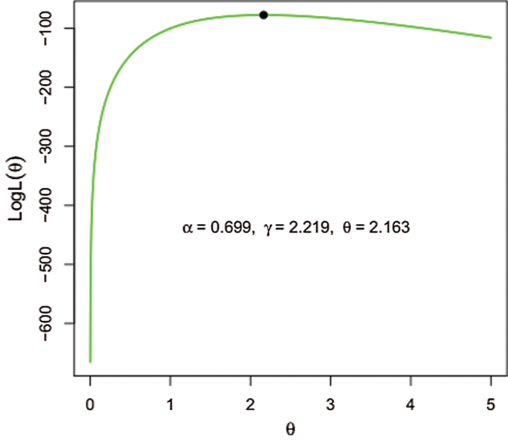
Figure 6: The log-likelihood as a function of θ.

6  Data Source and its Graphical Representation

The data set used in this study is representing the remission times of stomach cancer patients released by Cancer Research Foundation. These remission times and are used here only for illustrative purposes. The descriptive measures of the data are presented in Tab. 1.

Table 1: Descriptive measures of the stomach cancer patient’s data

The Kaplan–Meier survival plot of the data is sketched in Fig. 7.

Figure 7: The Kaplan–Meier survival plot of the stomach cancer patient’s data

From Fig. 7, it is clear, that the more time passes the more chance of survival decreases. The total time test (TTT) plot is an important graphical approach to check whether the data can be applied to a particular distribution or not. The TTT plot is used to check the behavior of the data to see whether the data has a monotonic or non-monotonic failure rate function. The hrf is said to be

•   Constant, if the TTT plot is graphically presented as a straight diagonal.

•   Increasing, if the TTT plot is concave.

•   Decreasing, if the TTT plot is convex.

•   U-shaped if the TTT plot is convex and then concave,

•   Unimodal, if the TTT plot is concave and then convex.

For further detail, we refer the interested readers to Aarset [17]. The TTT plot presented in Fig. 8, indicating that the bladder cancer data has a unimodal shaped failure rate.

Figure 8: The TTT plot of the stomach cancer patient’s data

7  Model Selection Criteria

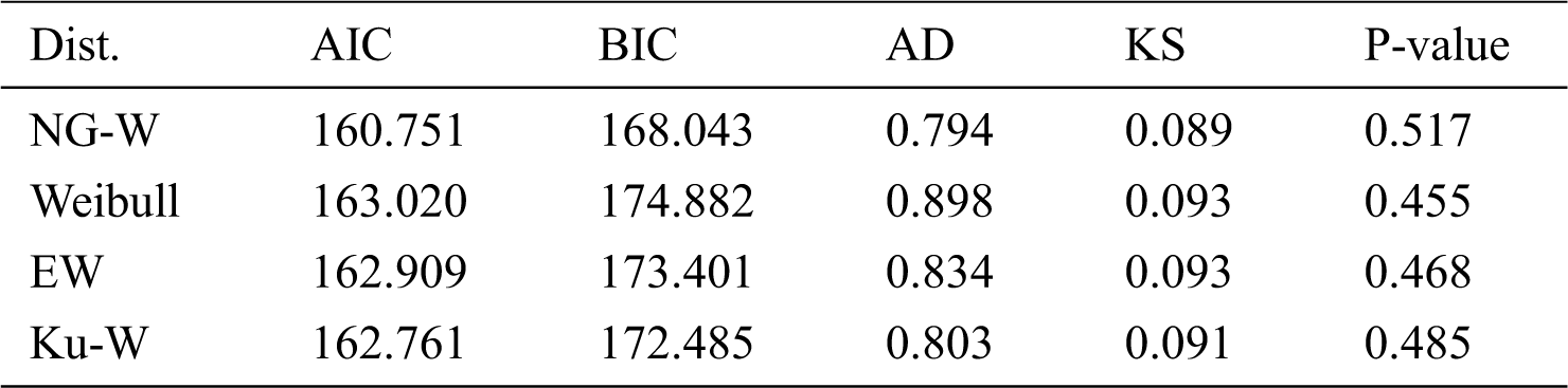
Model selection is one of the fundamental tasks of scientific inquiry to choose a statistical model from a group of candidate models. A number of statistical procedures are available to decide about the goodness of fit among the competing distributions. The most commonly used criteria are the (i) Akaike information criterion (AIC), (ii) Bayesian information criterion (BIC), (iii) Anderson Darling (AD) test statistic and (iv) Kolmogorov Simonrove (KS) test statistic with the corresponding p-value. A model with the lowest values for these statistics could be chosen as the best model to fit the data.

8  Application of the NG-W Model to the Stomach Cancer Data

In this section, we provide data analysis of the stomach cancer patient’s data to illustrate the NG-W model. We fit the proposed model to this data, and the comparison is made with the Weibull, Kumaraswamy–Weibull (Ku-W), and exponentiated Weibull (EW) models.

For the stomach cancer data, the MLEs with standard errors of the competing models are provided in Tab. 2. Whereas, values of the AIC, BIC, AD and KS statistics with p-values are presented in Tab. 3. From the results provided in Tab. 3, it is clear that the NG-W model could be chosen as the best model among the fitted models since the proposed model has the lowest values of the AIC, BIC, AD and KS. The analysis is performed via the optim() R-function with the argument method = “BFGS”.

Table 2: Estimated values with standard error (in parentheses) of the competing models

Table 3: Goodness of fit measures of the competing models

The plot of the distribution function of the NG-W distribution is displayed in Fig. 9. The plot sketched in Fig. 9, reveal that the NG-W model closely fits the stomach cancer patient’s data.

Figure 9: The fitted cdf for the stomach cancer data

9  Bayesian Estimation

Bayesian inference procedures have been taken into consideration by many statistical re- searchers, especially researchers in the field of survival analysis and reliability engineering. In this section, a complete sample data is analyzed through Bayesian point of view. We assume that the parameters α, γ and θ of NG-W distribution have independent prior distributions as

α∼Gamma(a,b),γ∼Gamma(c,d),θ∼Gamma(e,f),

where a,b,c,d,e and f are positive. Hence, the joint prior density function is formulated as follow:

π(α,γ,θ)=badcfeΓ(a)Γ(c)Γ(e)αα−1γc−1θe−1e−(bα+dγ+fθ). (15)

In the Bayesian estimation, the actual value of the parameter may be adversely affected by the loss when choosing an estimator. This loss can be measured by a function of the parameter and the corresponding estimator. Five well-known loss functions and associated Bayesian estimators and corresponding posterior risk are presented in Tab. 4.

Table 4: Bayes estimator and posterior risk under different loss functions

Next, we provide the posterior probability distribution for a complete data set. We define the function α as

φ(α,γ,θ)=αα−1γc−1θe−1e−(bα+dγ+fθ),α>0,γ>0,θ>0

The joint posterior distribution in terms of a given likelihood function L(data) and joint prior distribution π(α,γ,θ) id define as

π∗(α,γ,θ/data)∝π(α,γ,θ)L(data).. (16)

Hence, we get the joint posterior density of parameters α , γ and θ for complete sample data by combining the likelihood function and joint prior density provided in Eq. (16). Therefore, the joint posterior density function is given by

π∗(α,γ,θ/x_)=Kφ(α,γ,θ)∏i=1nθ2αγxiα−1e−γxiα(1−e−γxiα)θ−1log⁡(1+θ)(1+θ−θ(1−e−γxiα)θ), (17)

where K is given as

K−1=∫0∞∫0∞∫0∞φ(α,γ,θ)∏i=1nθ2αγxiα−1e−γxiα(1−e−γxiα)θ−1log⁡(1+θ)(1+θ−θ(1−e−γxiα)θ)dαdγdθ.

It is clear from Eq. (17) that there is no closed form for the Bayesian estimators under the five loss functions described in Tab. 4, so we suggest using a MCMC procedure based on 10000 replicates to compute Bayesian estimators. The corresponding Bayesian estimates and posterior risk are provided in Tab. 5. The 95% credible and HPD intervals for each parameter of the NG-W distribution are provided in Tab. 6. The posterior samples extracted by using the Gibbs sampling technique. Moreover, we provide the posterior summary plots in Figs. 10 and 11. These plots confirm that the sampling process is of the prime quality and the convergence does occur.

Table 5: Bayesian estimates and their posterior risks of the parameters under different loss functions based on the stomach cancer patient’s data

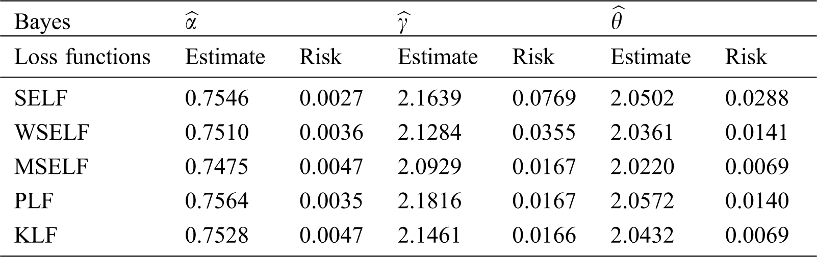
Table 6: Credible and HPD intervals of the parameters α , γ and θ for stomach cancer Patient’s data set

Figure 10: Plots of Bayesian analysis and performance of Gibbs sampling for the stomach cancer patient’s data set. Trace plots of each parameter of NG-W distribution

Figure 11: Plots of Bayesian analysis and performance of Gibbs sampling for the stomach cancer patients data set. Autocorrelation plots of each parameter of NG-W distribution

10  Concluding Remarks

In this article, we have introduced a new extension of the Weibull distribution, called a new generalized Weibull distribution. The classical two-parameter Weibull model produced simple monotone hazard shapes, as expected, that did not reect pattern of the unimodal hazard shape which is very important in biomedical research. On the other hand, the new extension of the Weibull model is capable to capture the unimodal hazard pattern. The proposed model along with the two-parameter Weibull, three-parameter exponentiated Weibull and four-parameter Kumaraswamy Weibull were applied to the remission times of the stomach cancer patient’s data. We observe that, in terms of the statistical significance of the model adequacy, suggesting that the NG-W model could play a reasonable role as a good candidate for modeling the stomach cancer data.

Funding Statement: School of Statistics, Shanxi University of Finance and Economics, Taiyuan china. (i) The National Social Science Fund of China (17BTJ010) and (ii) The Fund for Shanxi “1331 Project” Key Innovative ResearchTeam.

Conflicts of Interest: The authors declare that they have no conflicts of interest to report regarding the present study.

This work is licensed under a Creative Commons Attribution 4.0 International License, which permits unrestricted use, distribution, and reproduction in any medium, provided the original work is properly cited.