Computer Systems Science & Engineering DOI:10.32604/csse.2021.017144
Article

Efficient Concurrent L1-Minimization Solvers on GPUs

Xinyue Chu1, Jiaquan Gao1,*and Bo Sheng2

1Jiangsu Key Laboratory for NSLSCS, School of Computer and Electronic Information, Nanjing Normal University, Nanjing 210023, China
2Department of Computer Science, University of Massachusetts Boston, MA 02125, USA
*Corresponding Author: Jiaquan Gao. Email: springf12@163.com
Received: 20 January 2021; Accepted: 22 February 2021

Abstract: Given that the concurrent L1-minimization (L1-min) problem is often required in some real applications, we investigate how to solve it in parallel on GPUs in this paper. First, we propose a novel self-adaptive warp implementation of the matrix-vector multiplication (Ax) and a novel self-adaptive thread implementation of the matrix-vector multiplication (ATx), respectively, on the GPU. The vector-operation and inner-product decision trees are adopted to choose the optimal vector-operation and inner-product kernels for vectors of any size. Second, based on the above proposed kernels, the iterative shrinkage-thresholding algorithm is utilized to present two concurrent L1-min solvers from the perspective of the streams and the thread blocks on a GPU, and optimize their performance by using the new features of GPU such as the shuffle instruction and the read-only data cache. Finally, we design a concurrent L1-min solver on multiple GPUs. The experimental results have validated the high effectiveness and good performance of our proposed methods.

Keywords: Concurrent L1-minimization problem; dense matrix-vector multiplication; fast iterative shrinkage-thresholding algorithm; CUDA; GPUs

1  Introduction

Due to the sparsity of the solution of the L1-min problem, it has been successfully applied in various fields such as signal processing [1–3], machine learning [4–8], and statistical inference [9]. Moreover, the concurrent L1-min problem where a great number of L1-min problems need be concurrently computed is often required in these real applications. This motivates us to discuss the concurrent L1-min problem in this paper. Here the following concurrent L1-min problem is considered:

min||xi||1s.t.Axi=bi,i=1,2,⋯,k, (1)

where A∈Rm×n(m<<n) is a full-rank dense matrix, bi∈Rm is a pre-specified vector, and xi∈Rn is an unknown solution. Each one of these L1-min problems is independent except that they share the matrix A. This makes it suitable for parallel computing.

Given their multiple core structures, graphics processing units (GPUs) have sufficient computation power for scientific computations. Processing big data by GPUs has drown much attention over the recent years [10–14]. Following the introduction of the compute unified device architecture (CUDA), a programming model that supports the joint CPU/GPU execution of applications by NVIDIA [15], GPUs have become strong competitors as general-purpose parallel programming systems.

Due to high compute capacity of GPUs, accelerating algorithms that are used to solve the L1-min problem on the GPU has attracted considerable attention recently [16,17]. As we know, there exists a great number of L1-min algorithms such as the gradient projection method [18], truncation Newton interior-point method [19], homotopy methods [20], augmented Lagrange multiplier method (ALM) [21], class of iterative shrinkage-thresholding methods (FISTA) [22], and alternating direction method of multipliers [23]. And most of them are composed of dense matrix-vector multiplications such as Ax and ATx, and vector operations. In 2011, Nath et al. [24] presented an optimization symmetric dense matrix-vector multiplication on GPUs. In 2016, Abdelfattah et al. [25] proposed an open-source, high-performance library for the dense matrix-vector multiplication on GPU accelerators, KBLAS, which provides optimized kernels for a subset of Level 2 BLAS functionalities on CUDA-enabled GPUs. Moreover, a subset of KBLAS high performance kernels has been integrated into the CUBLAS library [26], starting from version 6.0. In addition, there have been highly efficient implementations for the vector operation on the GPU in the CUBLAS library. Therefore, the existing GPU-accelerated L1-min algorithms are mostly based on CUBLAS.

However, for the implementations of Ax and ATx in CUBLAS, the performance value fluctuates as m (row) increases when n (column) is fixed or n increases when m is fixed, and the difference between the maximum and minimum performance values is distinct. In [17], Gao et al. observe these phenomena, and present two novel Ax and ATx implementations on GPU to alleviate the drawbacks of CUBLAS. Furthermore, they take FISTA and ALM to propose two adaptive optimization L1-min solvers on GPU.

In this paper, we further investigate the design of effective algorithms that are used to solve the L1-min problem on GPUs. Different from other publications [16,17], here we emphasize the design of concurrent L1-min solvers on GPUs. First, we enhance Gao’s GEMV and GEMV-T kernels by optimizing the warp allocation strategy of the GEMV kernel and the thread allocation strategy of the GEMV-T kernel, and designing the optimization schemes for the GEMV and GEMV-T kernels. Second, the vector-operation and inner-product decision trees are established automatically to merge the same operations into a single kernel. For any-sized vector, the optimization vector-operation and inner-product implementation methods are automatically and rapidly selected from the decision trees. Furthermore, the popular L1-min algorithm, fast iterative shrinkage-thresholding algorithm (FISTA), is taken for example. Based on the proposed GEMV, GEMV-T, vector-operation and inner-product kernels, we present two optimization concurrent L1-min solvers on a GPU that are designed from the perspective of the streams and the thread blocks, respectively. Finally, we design a concurrent L1-min solver on multiple GPUs. In this solver, each GPU only solves a L1-min problem every time instead of solving multiple L1-min problems by utilizing multiple streams or thread blocks. This solver is applied to this case where the number of L1-min problems included in the concurrent L1-min problem is much less than the number of streams (or thread blocks). Experimental results show that our proposed GEMV and GEMV-T kernels are more robust than those that are suggested by Gao et al. and CUBLAS, and the proposed concurrent L1-min solvers on GPUs are effective. The main contributions are summarized as follows:

•   Two novel adaptive optimization GPU-accelerated implementations of the matrix-vector multiplication are proposed.

•   Two optimization concurrent L1-min solvers on a GPU are presented from the perspective of the streams and thread blocks, respectively.

•   Utilizing new features of GPU and the technique of merging kernels, an optimization concurrent L1-min solver on multiple GPUs is proposed.

The remainder of this paper is organized as follows. In Section 2, we describe the fast iterative shrinkage-thresholding algorithm. Two adaptive optimization implementations of the matrix-vector multiplication on the GPU and the vector-operation and inner-product decision trees are described in Section 3. Sections 4 and 5 give two concurrent L1-min solvers on a GPU and a concurrent L1-min solver on multiple GPUs, respectively. Experimental results are presented in Section 6. Section 7 contains our conclusions and points to our future research directions.

2  Fast Iterative Shrinkage-Thresholding Algorithm

The L1-min problem is known as the basis pursuit (BP) problem [27]. In practice, a measurement data b often contains noise (such as the measurement error: ε ), which is called the BPDN problem. A variant of this problem is also well known as the unconstrained BPDN problem with a scalar weight λ or the Lasso problem [28] in the statistics perspective:

min12||Ax−b||22+λ||x||1. (2)

The fast iterative shrinkage-thresholding algorithm (FISTA) is a kind of accelerations, and achieves an accelerated non-asymptotic convergence rate of O(k2) by combining Nesterov’s optimal gradient method [22]. For FISTA, it adds a new sequence {yk,k=1,2,⋯} as follows.

{xk+1=soft(yk−1Lf∇f(yk),λLf),tk+1=1+1+4tk22,yk+1=xk+tk−1tk+1(xk−xk−1), (3)

where soft(u,a)=sign(u)max{|u|−a,0} is the soft-thresholding operator, y1=x0 , t1=1 and the associated Lipschitz constant Lf of ∇f(⋅) is given by the spectral norm of ATA, denoted by ||ATA||2 . For large-scale problems, Lf is not always easily computable. Thus, a backtracking stepsize rule is suggested to alleviate this drawback. Algorithm 1 summarizes the generic FISTA algorithm with a backtracking stepsize rule [22].

3  GPU Kernels

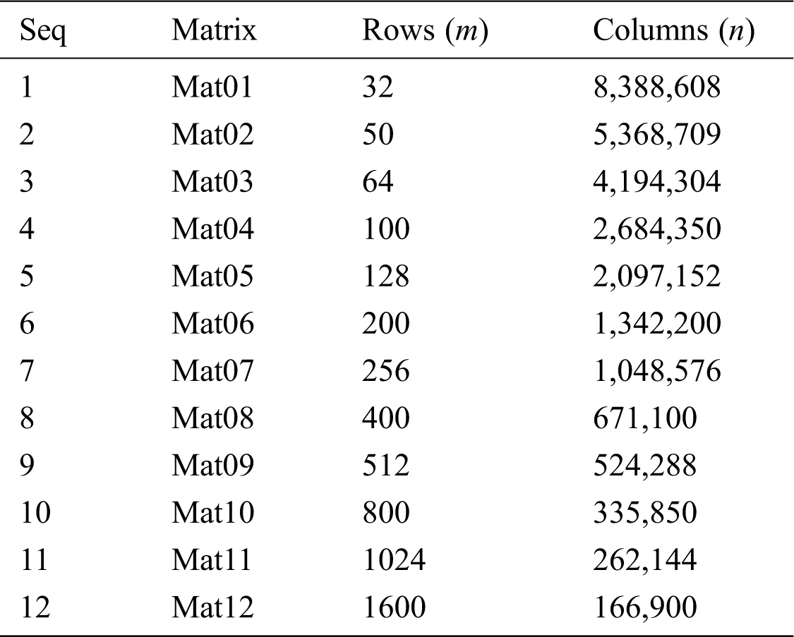
For FISTA, its main components include Ax (GEMV) and ATx (GEMV-T), vector operations, and inner product of vector. In the following subsection, we present their implementations on the GPU, respectively. Tab. 1 lists the symbols that are used in this paper. Nsm , Nreg , Nmem , Ntb , and Ntd are constants for a specific GPU. A row major and 0-based indexing array a is used to store the matrix A and the float precision values are only used for all computations in this paper.

Table 1: Symbols used in this paper

3.1 GEMV Kernel

Given that the GEMV, Ax, is composed of dot products of x and Ai (the ith row of A), i=1,2,⋯,m , and these dot products can be independently computed, we assign one warp or multiple warps to a product dot for our proposed GEMV kernel. To optimize the GEMV kernel performance, for a given nt, we propose the following self-adaptive warp allocation strategy to select the number of warps k for a product dot:

maxk=Nsm×Nmb×nt/nt32/32ww32/32ww,s.t. (4)

m≤w, (5)

k≤nt/nt3232andk=2z,z∈{0,1,2,⋯}. (6)

Eq. (4) denotes the objective of maximizing the number of warps. Eq. (5) guarantees that each warp group (k warps are grouped into a warp group) calculates at least a product dot. Eq. (6) guarantees that k must be a power of two and the warp-group size is at most the number of threads per block. Nmb in Eq. (4) is calculated as follows:

Nmb=min(Nreg/NregNbregNbreg,Nmem/NmemNbmem,Ntd/NtdntntNbmem,Ntd/Ntdntnt,Ntb), (7)

where Nbreg and Nbmem denote the number of registers and the amount of shared memory required by the threads per block for our proposed GEMV kernel, respectively. Here Nmb is the minimum number of blocks per grid that maximize the resource utilization per multiprocessor. In this paper, we take Nsm×Nmb as nb.

The GEMV kernel is mainly composed of the following three steps:

1.    x-load step: The step is used to make threads per block parallel read x into the shared memory xS. Because the size of x is large, x is segmentally read into the shared memory. To take full advantage of the amount of shared memory per multiprocessor, the size of shared memory per block is set as follows:

SIZE−MEM=Nmem/NmemNmb/Nmb44Nmb/Nmb44, (8)

where Nmb is calculated by Eq. (7). The time of loading x is xTimes=n/SIZE_MEM . By this way, the accesses to x are coalesced, and the access number is reduced by letting threads in the same thread block to share the section of elements of x.

2.    Partial-Reduction Step: Each time after a section of elements of x is read into the shared memory, the threads in each warp group perform in parallel a partial-style reduction. Obviously, each thread in a warp group at most performs n/SIZE_WG times of reductions and the accesses to the global memory a are coalesced. Here SIZE_WG is the number of threads in the warp group, and is equal to k × 32.

3.    Warp-Reduction Step: After the threads in each warp group have completed the partial-style reductions, the fast shuffle instructions are utilized to perform a warp-style reduction for each warp in these warp groups. The warp-style reduction values are stored in the shared memory. Then the warp-style reduction values in the shared memory for each warp group are reduced to an output value in parallel.

3.2 GEMV-T Kernel

The GEMV-T, ATx, is composed of dot products of x and (AT)i (the ith column of A), i=1,2,⋯,n , and these dot products can be independently computed. Given that the size of the vector x in the GEMV-T is small, we assign one thread or multiple threads to a dot product in our proposed GEMV-T kernel. To optimize the GEMV-T kernel performance, for a given nt, we propose the following self-adaptive thread allocation strategy to select the number of threads k for a product dot:

maxk=Nsm×Nmb×2×nt/2×ntww,s.t. (9)

n≤w, (10)

k≤32andk=2z,z∈{0,1,2,⋯}. (11)

Eq. (9) denotes the objective of maximizing the number of threads. Eq. (10) guarantees that each thread group (k threads are grouped into a thread group) calculates at least a product dot. Eq. (11) guarantees that k must be a power of two and the thread-group size is at most the size of a warp. Nmb in Eq. (9) is calculated by the same equation as Eq. (7) except that Nbreg and Nbmem denote the number of registers and the amount of shared memory required by the threads per block for our proposed GEMV-T kernel. To maximize the resource utilization per multiprocessor, we take Nsm×Nmb as nb.

Similar to the GEMV kernel, our proposed GEMV-T kernel is also composed of the x-load step, partial-reduction step and warp-reduction step.

1.    x-load step: Like the GEMV kernel, this step is used to make threads per block parallel read elements of x into the shared memory xS. Given that the size of x is small, x is once read into the shared memory in the GEMV-T kernel.

2.    partial-reduction step: Since a row major and 0-based index format is used to store the matrix A, the accesses to A will not be coalesced if the thread groups are constructed in an inappropriate way. For example, we assume that A is a 4×8 matrix as shown in Fig. 1, 16 threads in a thread block are launched, and 2 threads are assigned to a dot product in the GEMV-T kernel. If we use the following thread groups {0,1},{2,3},{4,5},⋯,{14,15} , the accesses to A will not be coalesced. However, when the thread groups {0,8},{1,9},{2,10},⋯,{7,15} are utilized, the accesses to A are coalesced, as shown in Fig. 1b. Therefore, in the partial-reduction step, the thread groups are created according to Definition 3.1 below in order to ensure that the accesses to A are coalesced.

Figure 1: Access to A

Definition 3.1: Assume that the size of the thread block is s, h threads are assigned to a dot product in ATx, and z=s/h . The thread groups are created as follows {0,z,⋯,(h−1)×z} , {1,z+1,⋯,(h−1)×z+1} , ⋯ , {z−1,2×z−1,⋯,2×(h−1)×z−1} .

For these elements of x that are read into the shared memory, the threads in each thread group perform in parallel a partial-style reduction similar to that in the GEMV kernel.

3. warp-reduction step: These threads in a thread group are usually not in the same warp, so we cannot use the shuffle instruction to reduce their partial-style reduction values. Therefore, in the warp-reduction stage, we store the partial-style reduction values that are obtained by threads in each thread group to the shared memory, and then reduce them in the shared memory to an output value in parallel.

3.3 Vector-Operation and Inner-Prodcut Kernels

When parallelizing FISTA on the GPU, the vector-operation and inner-product kernels are needed. Although CUBLAS has shown good performance for the vector operations and the inner product of vector, the use of CUBLAS does not allow to group several operations into a single kernel. Here in order to optimize these operations, we try to group several operations into a single kernel. Therefore, we adopt the idea of constructing the vector-operation and inner-product decision trees that are suggested by Gao et al. [29]. Utilizing the vector-operation and inner-product decision trees, the optimal vector-operation and inner-product kernels and their corresponding CUDA parameters can be obtained. For readers that are interested in this work, please refer to the publication [29].

3.4 Optimization

Assume that s=Nsm×Nmb×nt/nt3232 , where Nmb is calculated by Eq. (7), and m=l+s+Δs , where l = 0, 1, 2, ⋯ , and Δs is a smaller positive integer than s. We observe that for a matrix with m=2×960+30 and n = 102,400 on the GTX 1070 GPU, nt = 1,024, the GEMV kernel with one warp per row is utilized according to Eq. (4), and thus achieves 103.18 GFLOPS. Let us divide this matrix into two blocks B(m=2×960,n=102,400) and C(m=30,n=102,400) . If B and C are calculated by one warp per row and 32 warps per row, respectively, we will obtain 107.25 GFLOPS. In this way, the performance of the GEMV kernel increases 4.07 GFLOPS. Why? Obviously, for the GEMV kernel, if Δs=0 and l > 0, each warp will calculate the same number of rows and thus it obtains good performance. However, when Δs≠0 and l > 0, the performance of the GEMV kernel decreases because many warps are idle when computing the remaining Δs rows. Based on the above observations, we optimize the GEMV kernel as follows.

•   When Δs=0l>0 or Δs≠0l=0 , the GEMV kernel shown in Section 3.1 is applied.

•   Otherwise, on the basis of the GEMV kernel, we construct a new kernel GEMV Kernel-I to calculate the GEMV on the GPU. In this kernel, each row of the first l×s rows is assigned to one warp, and each row of the last Δs rows is calculated by self-adaptive multiple warps.

Similar to the GEMV kernel, for the GEMV-T kernel, we assume that s=Nsm×Nmb×nt and m=l+s+Δs , where l = 0, 1, 2, ⋯ , and Δs is a smaller positive integer than s, and then optimize it as follows.

•   When Δs=0l>0 or Δs≠0l=0 , the GEMV kernel shown in Section 3.2 is applied.

•   Otherwise, on the basis of the GEMV-T kernel, we construct a new kernel GEMV-T Kernel-I to calculate the GEMV on the GPU. In this kernel, each row of the first l×s rows is assigned to one thread, and each row of the last Δs rows is calculated by self-adaptive multiple threads.

4  Concurrent L1-min Solvers on a GPU

In this section, based on FISTA, we present two concurrent L1-min solvers on a GPU, which are designed from the perspective of the streams and the thread blocks, respectively.

4.1 Streams

Utilizing the multi-steam features of GPU, on the basis of FISTA, we design a concurrent L1-min solver, called CFISTASOL-SM, to solve the concurrent L1-min problem. Given that these L1-problems that are included in the concurrent L1-min problem can be independently computed, each one of them is assigned to a stream in the proposed CFISTASOL-SM. Fig. 2 shows the parallel framework of CFISTASOL-SM, which defines the following contents: 1) illustrating the tasks of the CPU and the stream, 2) listing the execution steps of CFISTASOL-SM on each stream, and 3) designating which operations should be grouped into a single kernel.

Figure 2: Parallel framework of CFISTASOL-SM

For temp=Ayk−b,∇f(yk)=ATtemp , and zk=Axk+1 in Fig. 2, they are easy to be implemented on the basis of our proposed GEMV and GEMV-T implementation methods on the GPU. The optimal vector-operation and inner-product kernels and their corresponding CUDA parameters are chosen by using the vector-operation and inner-product decision trees.

4.2 Thread Blocks

For a specific GPU, the maximum thread blocks can be calculated as TBs=Nsm×Ntb. Utilizing the features of multiple thread blocks, based on FISTA, we present a concurrent L1-min solver, called CFISTASOL-TB, to solve the concurrent L1-min problem. In CFISTASOL-TB, a L1-min problem is assigned to one thread block. For each thread block, the idea of constructing the parallel FISTA to solve the L1-min problem is similar to that of implementing FISTA on the stream in Section 4.1 except that here CFISTASOL-TB is implemented in a kernel.

4.3 Optimization

When the ith element of x is equal to zero, all elements in the ith column of A do not need to be accessed because they do not have any contribution to the output vector. With the increasing iteration in FISTA, x becomes sparser and sparser, and thus many columns in A are not accessed. By this way, we can improve the CFISTASOL-SM and CFISTASOL-TB performance by reducing accesses to the global memory a. Furthermore, for CFISTASOL-TB and CFISTASOL-SM, each thread block needs to access the global memory a, so we let a be cached in the read-only data cache in order to reduce the number of accesses to a. With the read-only data cache, a is shared by all thread blocks and can be accessed fast.

5  Concurrent L1-min Solver on Multiple GPUs

For the concurrent L1-min problem, if it includes a great number of L1-min problems, we can easily construct a solver on multiple GPUs to solve it by letting each GPU execute CFISTASOL-SM or CFISTASOL-TB. However, here we design a concurrent L1-min solver on multiple GPUs, called CFISTASOL-MGPU, where each GPU only solves a L1-min problem every time instead of solving multiple L1-min problems by utilizing the streams and the thread blocks. This solver is applied to this case where the number of L1-min problems that are included in the concurrent L1-min problem is much less than the number of the streams or the thread blocks. Fig. 3 shows the parallel framework of CFISTASOL-MGPU, which defines the following contents: 1) illustrating the CPU/GPU tasks, 2) listing the execution steps of CFISTASOL-MGPU on each GPU, and 3) designating which operations should be grouped into a single kernel. The operations in Fig. 3 are easily executed on each GPU using the kernels in Section 3.

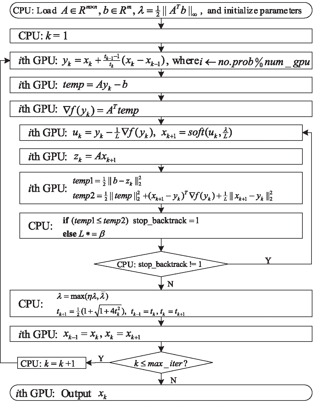
Figure 3: Parallel framework of CFISTASOL-MGPU

6  Performance Evaluation and Analysis

In this section, we first investigate the effectiveness of our proposed GEMV and GEMV-T kernels by comparing them with GEMV and GEMV-T implementations in the CUBLAS library [26] and those that are presented by Gao et al. [17]. Second, we test the performance of our proposed concurrent L1-min solvers on a GPU, CFISTASOL-SM and CFISTASOL-TB. Finally, we test the performance of our proposed concurrent L1-solver on multiple GPUs, CFISTASOL-MGPU. In the experiments, the number of threads per block is set to 1024 for all algorithms.

Tab. 2 shows NVIDIA GPUs that are used in the performance evaluations. Our source codes are compiled and executed using the CUDA toolkit 10.1. The measured GPU performance for all experiments does not include the data transfer (from the GPU to the CPU or from the CPU to the GPU). The test matrices, which come from the publication [17], are shown in Tab. 3. The elemental values of each test matrix are randomly generated according to the normal distribution. The performance is measured in terms of GFLOPS, which is obtained by 2×m×n the matrix-vector multiplication kernel execution time (the time unit is second) [30].

Table 2: Overview of GPUs

Table 3: Test matrices

6.1 Performance Evaluation and Analysis of Matrix-Vector Multiplications

First, we compare GEMV and GEMV-T kernels with the implementations in the CUBLAS library [26] and those that are presented by Gao et al. [17]. The test matrices are shown in Tab. 3. Figs. 4 and 5 show the performance comparison of the GEMV kernel with CUBLAS and that of Gao et al., respectively. From Fig. 4, we observe that our proposed GEMV kernel on K40c and GTX1070 is always advantageous over CUBLAS and that of Gao et al. for all test matrices. On K40c and GTX1070, the average performance ratios of the proposed GEMV kernel versus CUBLAS are 3.15× and 1.12 × , respectively, and those of the proposed GEMV kernel versus Gao’s GEMV kernel are 3.18 × and 1.19 × , respectively. For the proposed GEMV-T kernel, it outperforms CUBLAS and Gao’s GEMV-T kernel for all test matrices on all two GPUs, as shown in Fig. 5. On K40c and GTX1070, the average performance improvement is respectively 1.40 × and 1.05 × compared to CUBLAS, and is respectively 1.09 × and 1.02 × compared to Gao’s GEMV-T kernel. These observations verify the effectiveness of the proposed GEMV and GEMV-T kernels.

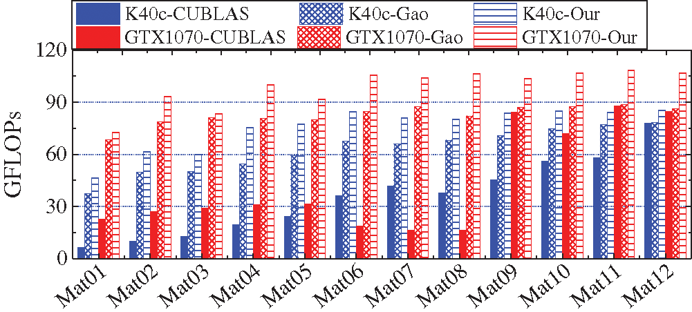
Figure 4: Performance comparison of GEMV kernels

Figure 5: Performance comparison of GEMV-T kernels

Second, we take GTX1070 to investigate whether can the proposed GEMV and GEMV-T kernels alleviate the CUBLAS fluctuations? The test matrix sets are as follows: 1) Set 1: n = 100,000 and m = 50, 100, 150, ⋯ , 5,000; 2) Set 2: m = 1,000 and n = 5,000, 10,000, 15,000, ⋯ , 500,000.

Figs. 6 and 7 show the performance curves of GEMV and GEMV-T kernels for the matrices in the two sets, respectively. From Fig. 6, we observe that whether m increases when n is fixed to 100,000 or n increases when m is fixed to 1,000, the CUBLAS performance fluctuates, and the difference between the maximum and minimum performance values is significant. However, for our proposed GEMV kernel, it is advantageous over CUBLAS, and its performance almost remains invariable, and always preserves around 107 GFLOPS for all cases. Furthermore, for the test matrices in Set 1, the performance of our proposed GEMV-T kernel has been maintained at around 107 GFLOPS as m increases, as shown in Fig. 7(a). However, the CUBLAS performance fluctuates as m increases. For the test matrices in Set 2, when n increases, our proposed GEMV-T kernel has high performance as CUBLAS, and always achieves around 107 GFLOPS.

Figure 6: GEMV (a) Performance curves with m (n = 100,000) (b) performance curves with n (m = 1,000)

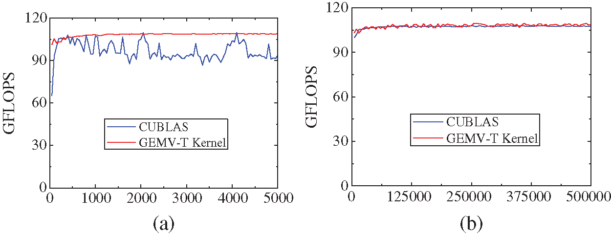
Figure 7: GEMV-T (a) Performance curves with m (n = 100,000) (b) performance curves with n (m = 1,000)

Based on the above observations, we conclude that our proposed GEMV and GEMV-T kernels enhance those that are suggested by Gao et al., and achieve high performance, and are able to alleviate the performance fluctuations of CUBLAS.

6.2 Performance of Concurrent L1-min Solvers on a GPU

In this section, we test the performance of our proposed CFISTASOL-TB and CFISTASOL-SM. Given that these L1-min problems included in the concurrent L1-min problem can be independently computed, as a comparison, we use the FISTA implementation on the CPU using the BLAS library (denoted by BLAS), the FISTA implementation using the CUBLAS library (denoted by CUBLAS), and the FISTA solver (denoted by GAO) that is proposed in [17] to calculate them. 12 test cases are applied. For each test case, 60 L1-min problems are concurrently calculated, and the matrix A comes from Tab. 3. For each L1-min problem, the initial x0 with 1024 non-zero elements is randomly generated according to the normal distribution, and b=Ax0 . All algorithms stop after the number of iterations is more than 100 for all test cases. Tabs. 4 and 5 show the execution time of all algorithms on a K40c and a GTX1070, respectively. The time unit is second (denoted by s ). In Tabs. 4 and 5, our proposed CFISTASOL-TB and CFISTASOL-SM are abbreviated as TB and SM, respectively.

Table 4: Execution time of all algorithms on a K40c (The time unit is s)

Table 5: Execution time of all algorithms on a GTX1070 (The time unit is s)

On two GPUs, both TB and SM outperform BLAS, CUBLAS and GAO for all test cases (Tabs. 4 and 5). On a K40c, the execution time ratios of CUBLAS to TB range from 4.18 to 33.28, and the average execution time ratio is 12.22; The execution time ratios of GAO to TB range from 3.92 to 6.52, and the average execution time ratio is 4.80; The minimum and maximum execution time ratios of CUBLAS to SM are 4.18 and 22.18, respectively, and the average execution time ratio is 11.04; The minimum and maximum execution time ratios of GAO to SM are 3.92 and 5.79, respectively, and the average execution time ratio is 4.54. Furthermore, we observe that TB is slightly better than SM in most cases. On a GTX1070, we obtain the same conclusion as on a K40c from Tab. 5. The average execution time ratios of CUBLAS versus TB and CUBLAS versus SM are 18.00 and 15.76, respectively, and the average execution time ratios of GAO versus TB and GAO versus SM are 7.24 and 6.38, respectively. Especially, compared to the solver on the CPU, BLAS, TB respectively obtains average speedups of 62.78 × and 126.16 × , and SM respectively obtains average speedups of 59.65 × and 110.99 × , on a K40c and a GTX1070 (Fig. 8). These observations verify that our proposed TB and SM have high performance and parallelism.

Figure 8: Speedups of TB and SM on a GPU

6.3 Performance of the Concurrent L1-min Solver on Multiple GPUs

We take two GPUs and four GPUs for example to test the performance of our proposed CFISTASOL-MGPU. The test setting is as same as in Section 6.2. Fig. 9 shows speedups of CFISTASOL-MGPU versus BLAS on the K40c and GTX1070 GPUs.

Figure 9: Speedups of CFISTASOL-MGPU on multiple GPUs

From Fig. 9, we can observe that the speedups of CFISTASOL-MGPU versus BLAS on the two K40c GPUs range from 30.53 to 50.97 for all test cases, and the average speedup is 39.69. On the four K40c GPUs, the speedups of CFISTASOL-MGPU versus BLAS range from 61.06 to 101.9 for all test cases, and the average speedup is 79.38. On the two GTX1070 GPUs, the minimum and maximum speedups of CFISTASOL-MGPU versus BLAS for all test cases are 49.7 and 64.81, respectively, and the average speedup is 54.22. On the four GTX1070 GPUs, the minimum and maximum speedups of CFISTASOL-MGPU versus BLAS for all test cases are 99.39 and 129.6, respectively, and the average speedup is 108.4. All observations show that CFISTASOL-MGPU is effective for solving the concurrent L1-min problem, and has high parallelism.

6.4 Discussion

From the experimental results, we can observe that CFISTASOL-TB is slightly better than CFISTASOL-SM, and CFISTASOL-SM is advantageous over CFISTASOL-MGPU. In fact, each one of these solvers has its own advantage. Tab. 6 lists the experimental results with different number of L1-min problems that are included in the concurrent L1-min problem on GTX1070. In this experiment, Mat12 is set as the coefficient matrix in the test concurrent L1-problem, and the test setting is as same as in Section 6.2. For the GTX1070, the maximum thread blocks that it launches is 30 when nt = 1024, the number of streams is 15. When the number of L1-min problems is enough to make all thread blocks busy, CFISTASOL-TB is better than other two algorithms (see the first problem in Tab. 6). Otherwise, CFISTASOL-SM will outperform other two algorithms if the number of L1-min problems is enough to make all streams busy (see the second problem in Tab. 6). When the number of L1-min problems is much more than the number of thread blocks and the number of streams, CFISTASOL-MGPU is the best of all three algorithms (see the third problem in Tab. 6). Therefore, we can get better algorithms by utilizing their own advantages to combine them. For example, on the four GTX1070 GPUs, assume that the number of L1-min problems that are included in the concurrent L1-min problem is 128, the first 120 problems are calculated in parallel by letting each GPU execute CFISTASOL-TB, and the remaining 8 problems are computed in parallel by executing CFISTASOL-MGPU.

Table 6: Execution time of algorithms (The time unit is s)

7  Conclusion

We investigate how to solve the concurrent L1-min problem in this paper, and present two concurrent L1-min solvers on a GPU and a concurrent L1-min solver on multiple GPUs. Experimental results show that our proposed concurrent L1-min solvers are effective, and have high parallelism.

Next, we will further do research in this field, and apply the proposed algorithms to more practical problems to improve them.

Funding Statement: The research has been supported by the Natural Science Foundation of China under great number 61872422, and the Natural Science Foundation of Zhejiang Province, China under great number LY19F020028.

Conflicts of Interest: We declare that there are no conflicts of interest to report regarding the present study.

References

 1.  J. Tropp, “Just relax: convex programming methods for subset selection and sparse approximation,” IEEE Trans. on Information Theory, vol. 52, no. 3, pp. 1030–1051, 2006. [Google Scholar]

 2.  A. Bruckstein, D. Donoho and M. Elad, “From sparse solutions of systems of equations to sparse modeling of signals and images,” SIAM Review, vol. 51, no. 1, pp. 34–81, 2009. [Google Scholar]

 3.  G. Ravikanth, K. V. N. Sunitha and B. E. Reddy, “Location related signals with satellite image fusion method using visual image integration method,” Computer Systems Science and Engineering, vol. 35, no. 5, pp. 385–393, 2020. [Google Scholar]

 4.  E. Elhamifar and R. Vidal, “Sparse subspace clustering: algorithm, theory, and applications,” IEEE Trans. on Pattern Analysis and Machine Intelligence, vol. 35, no. 11, pp. 2765–2781, 2013. [Google Scholar]

 5.  W. Sun, X. Zhang, S. Peeta, X. He and Y. Li, “A real-time fatigue driving recognition method incorporating contextual features and two fusion levels,” IEEE Trans. on Intelligent Transportation Systems, vol. 18, no. 12, pp. 3408–3420, 2017. [Google Scholar]

 6.  G. Zhang, H. Sun, Y. Zheng, G. Xia, L. Feng et al., “Optimal discriminative projection for sparse representation-based classification via bilevel optimization,” IEEE Trans. on Circuits and Systems for Video Technology, vol. 30, no. 4, pp. 1065–1077, 2020. [Google Scholar]

 7.  X. Zhang and H. Wu, “An optimized mass-spring model with shape restoration ability based on volume conservation,” KSII Trans. on Internet and Information Systems, vol. 124, no. 3, pp. 1738–1756, 2020. [Google Scholar]

 8.  X. Zhang, X. Yu, W. Sun and A. Song, “An optimized model for the local compression deformation of soft tissue,” KSII Trans. on Internet and Information Systems, vol. 14, no. 2, pp. 671–686, 2020. [Google Scholar]

 9.  J. Wright, Y. Ma, J. Mairal and G. Sapiro, “Sparse representation for computer vision and pattern recognition,” Proc. of the IEEE, vol. 98, no. 6, pp. 1031–1044, 2010. [Google Scholar]

10. L. He, H. Bai, D. Ouyang, C. Wang, C. Wang et al., “Satellite cloud-derived wind inversion algorithm using GPU,” Computers, Materials & Continua, vol. 60, no. 2, pp. 599–613, 2019. [Google Scholar]

11. Y. Guo, Z. Cui, Z. Yang, X. Wu and S. Madani, “Non-local dwi image super-resolution with joint information based on GPU implementation,” Computers, Materials & Continua, vol. 61, no. 3, pp. 1205–1215, 2019. [Google Scholar]

12. T. Chang, C. Chen, H. Hsiao and G. Lai, “Cracking of WPA & WPA2 using GPUs and rule-based method,” Intelligent Automation & Soft Computing, vol. 25, no. 1, pp. 183–192, 2019. [Google Scholar]

13. G. He, R. Yin and J. Gao, “An efficient sparse approximate inverse preconditioning algorithm on GPU,” Concurrency and Computation-Practice & Experience, vol. 32, no. 7, pp. e5598, 2020. [Google Scholar]

14. J. Gao, Q. Chen and G. He, “A thread-adaptive sparse approximate inverse preconditioning algorithm on multi-GPUs,” Parallel Computing, vol. 101, pp. 102724, 2021. [Google Scholar]

15. NVIDIA, “CUDA C Programming Guide v101. 2019. [Online]. Available at: http://docs.nvidia.com/cuda/cuda-c-programming-guide. [Google Scholar]

16. V. Shia, A. Yang, S. Sastry, A. Wagner and Y. Ma, “Fast l1-minimization and parallelization for face recognition,” in Conf. Record of the Forty Fifth Asilomar Conf. on Signals, Systems and Computers (ASILOMAR’11Piscataway, NJ: IEEE, pp. 1199–1203, 2011. [Google Scholar]

17. J. Gao, Z. Li, R. Liang and G. He, “Adaptive optimization 11-minimization solvers on GPU,” Int. Journal of Parallel Programming, vol. 45, no. 3, pp. 508–529, 2017. [Google Scholar]

18. M. Figueiredo, R. Nowak and S. Wright, “Gradient projection for sparse reconstruction: application to compressed sensing and other inverse problem,” IEEE Journal of Selected Topics in Signal Processing, vol. 1, no. 4, pp. 586–597, 2007. [Google Scholar]

19. S. Kim, K. Koh, M. Lustig, S. Boyd and D. Gorinevsky, “An interior-point method for large-scale 1-regularized least squares,” Int. Journal of Parallel Programming, vol. 1, no. 4, pp. 606–617, 2007. [Google Scholar]

20. D. Donoho and Y. Tsaig, “Fast solution of l1-norm minimization problem when the solution may be sparse, Stanford University, Technical Report, 2006. [Google Scholar]

21. A. Yang, Z. Zhou, A. Balasubramanian, S. Sastry and Y. Ma, “Fast l1-minimization algorithms for robust face recognition,” IEEE Transactions on Image Processing, vol. 22, no. 8, pp. 3234–3246, 2013. [Google Scholar]

22. A. Beck and M. Teboulle, “A fast iterative shrinkage-thresholding algorithm for linear inverse problems,” SIAM Journal on Imaging Sciences, vol. 2, no. 1, pp. 183–202, 2009. [Google Scholar]

23. B. Stephen, P. Neal and C. Eric, “Distributed optimization and statistical learning via the alternating direction method of multipliers,” Foundations and Trends in Machine Learning, vol. 3, no. 1, pp. 1–122, 2011. [Google Scholar]

24. R. Nath, S. Tomov, T. Dong and J. Dongarra, “Optimizing symmetric dense matrix-vector multiplication on GPUs,” in Proc. of 2011 Int. Conf. on High Performance Computing, Networking, Storage and Analysis (SC’11ACM, New York, NY, USA, pp. 1–10, 2011. [Google Scholar]

25. A. Abdelfattah, D. Keyes and H. Ltaief, “KBLAS: An optimized library for dense matrix-vector multiplication on GPU accelerators,” ACM Transactions on Mathematical Software, vol. 42, no. 3, pp. 1–31, 2016. [Google Scholar]

26. NVIDIA, “CUBLAS Library v10.1.” 2019. [Online]. Available at: http://docs.nvidia.com/cuda/cublas. [Google Scholar]

27. S. Chen, D. Donoho and M. Saunders, “Atomic decomposition by basis pursuit,” SIAM Journal on Scientific Computing, vol. 20, no. 1, pp. 33–61, 1998. [Google Scholar]

28. R. Tibshirani, “Regression shrinkage and selection via the lasso,” Journal of the Royal Statistical Society Series B, vol. 58, no. 1, pp. 267–288, 1996. [Google Scholar]

29. J. Gao, Y. Wang, J. Wang and R. Liang, “Adaptive optimization modeling of preconditioned conjugate on multi-GPUs,” ACM Transactions on Parallel Computing, vol. 3, no. 3, pp. 1–33, 2016. [Google Scholar]

30. J. Gao, Y. Zhou, G. He and Y. Xia, “A multi-GPU parallel optimization model for the preconditioned conjugate gradient algorithm,” Parallel Computing, vol. 63, pp. 1–16, 2017. [Google Scholar]

This work is licensed under a Creative Commons Attribution 4.0 International License, which permits unrestricted use, distribution, and reproduction in any medium, provided the original work is properly cited.