Output Feedback Robust <i>H<sub>∞</sub></i> Control for Discrete 2D Switched Systems

Wenjun Gao; Yang Yang; Hongtao Duan; Mingsheng Li; Jinrong Ma; Songwei Jin

doi:10.32604/csse.2021.016475

Loading [MathJax]/jax/output/CommonHTML/jax.js

[BACK]

Computer Systems Science & Engineering DOI:10.32604/csse.2021.016475
Article

Output Feedback Robust H∞ Control for Discrete 2D Switched Systems

Wenjun Gao1, Yang Yang1,*, Hongtao Duan1, Mingsheng Li1, Jinrong Ma1 and Songwei Jin2

1School of Electronic Information and Engineering, Changchun University of Science and Technology, Changchun, 130000, China
2Department of Computer Science and Engineering, University of California, Riverside, CA92521, USA
*Corresponding Author: Yang Yang. Email: cloneyang@126.com
Received: 03 January 2021; Accepted: 17 February 2021

Abstract: The two-dimensional (2-D) system has a wide range of applications in different fields, including satellite meteorological maps, process control, and digital filtering. Therefore, the research on the stability of 2-D systems is of great significance. Considering that multiple systems exist in switching and alternating work in the actual production process, but the system itself often has external perturbation and interference. To solve the above problems, this paper investigates the output feedback robust H∞ stabilization for a class of discrete-time 2-D switched systems, which the Roesser model with uncertainties represents. First, sufficient conditions for exponential stability are derived via the average dwell time method, when the system’s interference and external input are zero. Furthermore, in the case of introducing the external interference, the weighted robust H∞ disturbance attenuation performance of the underlying system is further analyzed. An output feedback controller is then proposed to guarantee that the resulting closed-loop system is exponentially stable and has a prescribed disturbance attenuation level γ. All theorems mentioned in the article will also be given in the form of linear matrix inequalities (LMI). Finally, a numerical example is given, which takes two uncertain values respectively and solves the output feedback controller’s parameters by the theorem proposed in the paper. According to the required controller parameter values, the validity of the theorem proposed in the article is compared and verified by simulation.

Keywords: 2-D systems; robust H∞ control; LMI; output feedback; switched systems; Roesser model

1 Introduction

The issue of stability analysis and controller synthesis is a hot research topic. Reference Medvedeva et al. [1–3] investigated the stability of one-dimensional (1-D) continuous-time or discrete-time systems. Considering the complexity of many manufacturing processes and physical phenomena, a 2-D continuous-time or discrete-time system that depends on two independent variables has its irreplaceable application area. 2-D systems have attracted considerable research attention in control theory and practice over the past few decades due to their wide applications. Reference Du et al. [4–7] showed multi-dimensional digital filtering, linear image processing, signal processing, and process control. Different models such as the Roesser model and Fornasini–Marchesini model can represent 2-D systems, and the stability issues concerning these two models can be found [8,9].

On the other hand, considerable interest has been devoted to the research of switched systems during the recent decades. A switched system comprises a family of subsystems described by continuous or discrete-time dynamics and a switching law that specifies the active subsystem at each instant of time. The switching strategy improves control performance [10–13] and arise many engineering applications, such as in motor engine control, constrained robotics, and satellite image control systems [14]. As far as time-dependent switching is concerned, the average dwell time (ADT) switching is employed in most references owing to its flexibility [15,16].

However, perturbations and uncertainties widely exist in practical systems. In some cases, the perturbations can be merged into the disturbance, which can be bounded in the appropriate norms. The main advantage of robust H∞ control is that its performance specification considers the system’s worst-case performance in terms of energy gain. This is more appropriate for system robustness analysis and robust control under modeling disturbances than other performance specifications. Recently, the problems of robust H∞ control and filtering for 2-D systems have been studied by many researchers [17–20], and so do the same problems of switched systems [21–23]. However, to the best of our knowledge, the output feedback robust H∞ control problem of 2-D switched systems in the Roesser model with uncertainties has not yet been thoroughly investigated, which motivates this present study.

In this paper, we confine our attention to the robust H∞ control problem of discrete 2-D switched systems described by the Roesser model with uncertainties. The main theoretical contributions are threefold: (1) We contribute to the development of stabilization for a class of 2-D switched systems that are exponentially stable, which the Roesser model with uncertainties represents. (2) A sufficient condition is presented to ensure a 2-D switched system’s exponential stability at a given disturbance attenuation level robust weighted H∞. (3) Based on the above two points, this article further designs the output feedback controller of the closed-loop system.

The paper is organized as follows. According to the current research results, we first study the exponential stability of 2-D switched systems described by the Roesser model with uncertainties. Further, when the system contains perturbations, we analyze the robust H∞ performance index of the system. Finally, we design an output feedback controller for the open-loop system, and an example is given to illustrate the effectiveness of the proposed method.

2 Notation

The following notations are used throughout the paper: the superscript “T” denotes the transpose, and the notation X ≥ Y (X > Y) means that matrix X − Y is positive semi-definite (positive definite, respectively). $‖⋅‖$ denotes the Euclidean norm. I represents the identity matrix. Diag ${ai}$ denotes a diagonal matrix with the diagonal elements ai, i = 1, 2,…,n. X-1 denotes the inverse of X. Rn denotes the n dimensional vector. Z+ represents the set of all non-negative integers. The l2 norm of a 2-D signal w(i,j) is given by $‖w‖2=∑i=0∞∑j=0∞‖w(i,j)‖2$ , where w(i,j) belongs to $l2{[0,∞),[0,∞)}$ .

3 Problem Formulation and Preliminaries

The uncertain Roesser model for a 2-D switched system $G:u→y$ is given by the following state equation:

$x¯(k,l)=Aδ(k,l)(Δ)x(k,l)+Bδ(k,l)w(k,l)z(k,l)=Cδ(k,l)x(k,l)+Dδ(k,l)w(k,l),k,l=0,1,2⋯$ (1)

with

$x¯(k,l)=[xh(k+1,l)xv(k,l+1)],x(k,l)=[xh(k,l)xv(k,l)]Aδ(k,l)(Δ)=Aδ(k,l)+Fδ(k,l)Gδ(k,l)(k,l)Hδ(k,l)$

where $Gδ(k,l)(k,l)$ is an unknown uncertain matrix and satisfies the norm bounded condition $GTδ(k,l)(k,l)Gδ(k,l)(k,l)≤I$ , and where $xh(k,l)∈Rn1$ and $xv(k,l)∈Rn2$ denote the system horizontal state and vertical state, respectively. Furthermore, $x(k,l)$ is the whole state in $Rn$ with $n=n1+n2$ , and $w(k,l)∈Rq$ is the interference input which belongs to $w(k,l)∈l2{[0,∞),[0,∞)}$ . $u(k,l)∈Rp$ and $z(k,l)∈Rq$ are control input and control output respectively; k and l are integers in Z. $δ(k,l):Z+×Z+→N={1,2,3⋯,N}$ is the switching signal. N is the number of subsystems. $δ(k,l)=i,i∈N$ denotes that the ith subsystem is activated., Ai, Bi, Ci, Di, Fi, Gi, Hi, are constant matrices with appropriate dimensions.

The boundary condition satisfies:

$X(0)=[xhT(0,0),xhT(0,1),⋯,xvT(0,0),xvT(1,0),⋯]T$ (2)

It is easy to know from the above formula $‖X(0)‖2<∞$ .

Remark 1. “In this paper, it is assumed that switching occurs only at each sampling point of k or l. The switching sequence can be described as

$((k0,l0),δ(k0,l0)),⋯,((kk,lk),δ(kk,lk)),⋯$ (3)

with $(kk,lk)$ denoting the kth switching instantly. It should be noted that the value of $δ(k,l)$ only depends on k+l [24,25].

Definition 1. System (1) is said to be exponentially stable under $δ(k,l)$ if for a given j ≥ 0, there exist positive constants c and f, such that

$∑k+l=D‖x(k,l)‖2≤fe−c(D−j)∑k+l=j‖x(k,l)‖r2$ (4)

holds for all D ≥ j [26].

Remark 2. From Definition 1, it is easy to see that when j is given, $∑k+l=j‖x(k,l)‖r2$ will be bounded, and $∑k+l=D‖x(k,l)‖r2$ will tend to be zero exponentially as D goes to infinity, which also means that $‖x(k,l)‖$ will tend to be zero exponentially.

Definition 2. For a given scalar $γ$ > 0, system (1) is said to have a weighted disturbance attenuation level $γ$ under switching signal $δ(k,l)$ if it satisfies the following conditions [4]:

(1) when $w(k,l)$ =0, system (1) is asymptotically stable or exponentially stable;

(2) under the zero-boundary condition, we have

$∑k=0∞∑l=0∞(ϕk+l‖z‖22)<γ2∑k=0∞∑l=0∞‖w‖22),∀0≠w(k,l)∈l2{[0,∞),[0,∞)}$ (5)

where 0 < $ϕ$ < 1 and the $l2$ -norm of 2D discrete signal $z(k,l)$ and $w(k,l)$ are defined as

$‖z‖22=‖z(k+1,l)‖22+‖z(k,l+1)‖22,‖w‖22=‖w(k+1,l)‖22+‖w(k,l+1)‖22$ (6)

Definition 3. For any $k+l=D≥j=kz+lz$ , let $Nδ(j,D)$ denote the switching number of $δ(⋅)$ on an interval $[z,D)$ . If

$Nδ(j,D)≤N0+D−jτa$ (7)

holds for given $N0≥0$ and $τa≥0$ , then the constant $τa$ is called the average dwell time and $N0$ is the chatter bound [27].

Lemma 1. For a given matrix $S=[S11S12S21S22]$ , where $S11$ and $S22$ are square matrices, the following conditions are equivalent [28].

$(i)S<0$ ;

$(ii)S11<0$ , $S22−S12TS11−1S12<0$ ;

$(iii)S22<0$ , $S11−S12S22−1S12T<0$ .

Lemma 2. Assuming that $x∈Rp,y∈Rq$ and $U,V,W$ are a suitable dimension matrix, then inequality $xTUVWy+yTWTVTUTx≤ε1xTUUTx+ε2yTWWTy$ is true for any $VTV≤I$ , if and only if there exist positive scalars $ε1,ε2$ and $ε1≥ε2$ .

Proof.

$0≤(ε1UTx−1ε1VWy)T(ε1UTx−1ε1VWy)=ε1xTUUTx−xTUVWy−yTWTVTUTx+1ε1yTWWTy≤ε1xTUUTx−xTUVWy−yTWTVTUTx+1ε2yTWWTy$

4 Exponential Stability Analysis

This section focuses on the exponential stability analysis of the 2D switched systems. The following theorem presents sufficient conditions that can guarantee that system (1) is exponentially stable.

Theorem 1. Consider 2D discrete switched system (1) with $w(k,l)=0$ , for a given positive constant $ϕ$ < 1, if there exist a set of positive-definite symmetric matrices $Pi∈Rn×n,i∈N$ and two positive scalars $ε1,ε2$ , such that

$[−ϕPiAiTPi0ε1HiTPiAi−PiPiFi00FiTPi−ε2I0ε1Hi00−ε1I]<0$ (8)

$ε1≥ε2$ (9)

Then, the system is exponentially stable for any switching signal with the average dwell time satisfying

$τa>τa∗=ln⁡μ−ln⁡ϕ$ (10)

where $μ$ ≥ 1 satisfies

$Pi≤μPj,∀i,j∈N$ (11)

Proof. Without loss of generality, we assume that the ith subsystem is active. For the ith subsystem, we consider the following Lyapunov function candidate:

$Vi(x(k,l))=xT(k,l)Pix(k,l)$ (12)

where $Pi$ is an $n×n$ positive-definite matrix for any $i∈N$ , and thus $Vi(x(k,l))>0,∀x(k,l)≠0$ and $Vi(k,l)=0$ only when $x(k,l)=0$ . Then we have $Vi(x¯(k,l))−ϕVi(x(k,l))=xT(k,l)(AiT(Δ)PiAi(Δ)−ϕPi)$ .

Using Lemma 1 to (8), we can get the equivalent inequality as follows:

$[−ϕPiAiTPi0ε1HiTPiAi−PiPiFi00FiTPi−ε2I0ε1Hi00−ε1I]<0⇒[−ϕPi+ε1HiTHiAiTPiPiAi−Pi+1ε2PiFiFiTPi]<0$

$⇒[−ϕPiAiTPiPiAi−Pi]+ε1[HiT0][Hi0]+1ε2[0PiFi][0FiTPi]<0$ (13)

Then using Lemma 2 to (13), we can get

$[−ϕPiAiTPiPiAi−Pi]+[HaiT0]GiT[0FiTPi]+[0PiFi]Gi[Hai0]<0$ (14)

Using Lemma 1 to (14), we can get

$AiT(Δ)PiAi(Δ)−ϕPi<0$ (15)

Form (15), we know

$Vi(x¯(k,l))≤ϕVi(x(k,l))$ (16)

The equality holds only if $Vi(x¯(k,l))=Vi(x(k,l))=0$ .

It follows from (16) that

$∑k+l=N+1Vi(k,l)≤ϕ∑k+l=NVi(k,l)≤ϕN−N0+1∑k+l=N0Vi(k,l)$ (17)

Now, let n = $Nδ(j,D)$ denote the switching number of $δ(⋅)$ on an interval $[j,D)$ , and let $mk−n+1<mk−n+2<⋯<mk−1<mk$ denote the switching points of $δ(⋅)$ over the interval $[j,D)$ , thus, for $D∈[mk,mk+1)$ , we have from (16)

$∑k+l=DVδ(mk)(k,l)<ϕD−mk∑k+l=mkVδ(mk)(k,l)$ (18)

Using (11) and (12), at switching instant $mk=k+l$ , we have

$∑k+l=mkVδ(mk)(k,l)≤μ∑k+l=mkVδ(mk−1)(k,l)$ (19)

Also, according to Definition 3, it follows that

$n=Nδ(j,D)≤N0+D−jτa$ (20)

Therefore, the following inequality can be obtained easily:

$∑k+l=DVδ(mk)(k,l)<ϕD−mk∑k+l=mkVδ(mk)(k,l)≤μϕD−mk∑k+l=mk−Vδ(mk−1)(k,l)<μϕD−mk∑k+l=mk−1Vδ(mk−1)(k,l)ϕmk−mk−1≤⋯<μn−1ϕD−mk−n+1∑k+l=mk−n+1Vδ(mk−n+1)(k,l)≤μnϕD−mk−n+1∑k+l=mk−n+1−Vδ(j)(k,l)<μnϕD−j∑k+l=jVδ(j)(k,l)$ (21)

Combining (20), inequality (21) can be written as follows:

$∑k+l=DVδ(mk)(k,l)≤e−(−ln⁡μτa−ln⁡ϕ)(D−j)∑k+l=jVδ(j)(k,l)$ (22)

There exist two positive constants a and b (a ≤ b) such that

$∑k+l=D‖x(k,l)‖2≤bae−(−ln⁡μτa−ln⁡ϕ)(D−j)∑k+l=j‖x(k,l)‖2$ (23)

By Definition 1, we know that if $−ln⁡μτa−ln⁡ϕ$ >0, that is $τa>τa∗=ln⁡μ−ln⁡ϕ$ , the 2D discrete switched system is exponentially stable.

The proof is completed.

Remark 3. Note that when $μ=1$ in (10), (11) turns out to be $Pi=Pj,∀i,j∈N$ . In this case, we have

$τa>τa∗=ln⁡μ−ln⁡ϕ$ , which means that the switching signal can be arbitrary.

5 Robust H∞ Performance Analysis

This section focuses on the Robust H∞ stabilization problem for a class of discrete-time 2D switched systems represented by a Roesser model with uncertainties. The following theorem presents sufficient conditions that can guarantee that system (1) is exponentially stable and has a prescribed weighted H∞ disturbance attenuation level $γ$ .

Theorem 2. For given positive scalars $γ$ and $ϕ$ < 1, there exist symmetric and positive-definite matrices $Pi∈Rn×n,i∈N$ , and two positive scalars $ε1,ε2$ ,such that

$[−ϕPi0AiTPi0CiTε1HiT0−γ2BiTPi0DiT0PiAiPiBi−PiPiFi0000FiPi−ε2I00CiDi00−I0ε1Hi0000−ε1I]<0$ (24)

$ε1≥ε2$ (25)

Then, 2D switched system (1) is exponentially stable and has a prescribed weighted H∞ disturbance attenuation level $γ$ for any switching signals with average dwell time satisfying (10), where μ ≥ 1 satisfies (11).

Proof. It is an obvious fact that (24) implies that inequality (8) holds. By Lemma 2, we can find that system (1) is exponentially stable when $w(k,l)$ = 0. Now we are able to prove that system (1) has a prescribed weighted H∞ performance γ for any nonzero $w(k,l)∈l2{[0,∞),[0,∞)}$ .

To establish the weighted H∞ performance, we choose the same Lyapunov functional candidate as in (12) for the system (1). Following the proof line of Theorem 1, we can get

$Vi(x¯(k,l))≤ϕVi(x(k,l))+γ2wTw−zTz$

$Φ=[AiT(Δ)PiAi(Δ)−ϕPi+CiTCiAiT(Δ)PiBi+CiTDiBiTPiAi(Δ)+DiTCiBiTPiBi−γ2+DiTDi]<0$ (26)

Using Lemma 1 to (26), we can get the equivalent inequality as follows:

$[−ϕPi+CiTCiCiTDiAiT(Δ)DiTCi−γ2+DiTDiBiTAi(Δ)Bi−(Pi)−1]<0⇔[−ϕPi+CiTCiCiTDiAiTDiTCi−γ2+DiTDiBiTAiBi−(Pi)−1]+[HaiT00]GiT[00FiT]+[00Fi]Gi[Hai00]<0$ (27)

Pre- and post-multiplying (24) by $diag{II(Pi)−1III}$ , we obtain

$[−ϕPi0AiT0CiTε1HiT0−γ2BiT0DiT0AiBi−(Pi)−1Fi0000Fi−ε2I00CiDi00−I0ε1Hi0000−ε1I]<0$ (28)

Using Lemma 1 to (28), we can get

$[−ϕPi+CiTCi+ε1HaiTHaiCiTDiAiTDiTCi−γ2+DiTDiBiTAiBi−(Pi)−1+1ε2FiFiT]<0$ (29)

Then using Lemma 2, we find that (29) is equivalent to (27).

Thus it can be obtained from (24) that

$Vi(x¯(k,l))−ϕVi(x(k,l))+γ2wTw−zTz<0$ (30)

Then we have

$Vi(x¯(k,l))≤ϕVi(x(k,l))+γ2wTw−zTz$ (31)

Let

$F(k+l)=‖z‖22−γ2‖w‖22=‖zh(k,l)zv(k,l)‖22−γ2‖wh(k,l)wv(k,l)‖22$ (32)

Summing up both sides of (31) from (D-1) to 0 with respect to l and 0 to (D-1) with respect to k, respectively, and applying the zero-boundary condition, one gets

$∑k+l=DVδ(mk)(k,l)<ϕD−1∑k+l=D−1Vδ(mk)(k,l)−∑k+l=D−1F(k,l)<ϕD−mk∑k+l=mkVδ(mk)(k,l)−∑m=mkD−1∑k+l=mϕD−1−k−lF(k,l)≤μϕD−mk∑k+l=mk−Vδ(mk−1)(k,l)−∑m=mkD−1∑k+l=mϕD−1−k−lF(k,l)<μϕD−(mk−−1)∑k+l=mk−−1Vδ(mk−1)(k,l)−μϕD−mk∑k+l=mk−−1F(k,l)−∑m=mkD−1∑k+l=mϕD−1−k−lF(k,l)<μNδ(k+l,D)ϕD−(mk−−1)∑k+l=mk−−1Vδ(mk−1)(k,l)−μNδ(k+l,D)∑m=mk−−1D−1∑k+l=mϕD−1−k−lF(k,l)<μNδ(k+l,D)ϕD−(mk−−1)∑k+l=mk−1Vδ(mk−1)(k,l)−μNδ(k+l,D)∑m=mk−1D−1∑k+l=mϕD−2−k−lF(k,l)≤μNδ(k+l−1,D)ϕD−mk−1∑k+l=mk−1−Vδ(mk−2)(k,l)−∑m=mk−1−D−1∑k+l=mμNδ(k+l+1,D)ϕD−1−k−lF(k,l)⋯<∑k+l=0μNδ(k+l,D)ϕDVδ(1)(k,l)−∑m=0D−1∑k+l=mμNδ(k+l,D)ϕD−1−k−lF(k,l)$ (33)

Under the zero-initial condition, we have

$∑k+l=0μNδ(k+l,D)ϕDVδ(1)(k,l)=0$ (34)

Thus, we have

$∑m=0D−1∑k+l=mμNδ(k+l,D)ϕD−1−k−lF(k,l)<−∑k+l=DVδ(mk)(k,l)$ (35)

Multiplying both sides of (35) by $μ−Nδ(0,D)$ , we can get the following inequality:

$∑m=0D−1∑k+l=mμ−Nδ(0,k+l)ϕD−1−k−l‖z‖22<γ2∑m=0D−1∑k+l=mμ−Nδ(0,k+l)ϕD−1−k−l‖w‖22$ (36)

Noting $Nδ(0,k+l)≤k+lτa$ , and using (10), we have

$μ−Nδ(0,k+l)=eμ−Nδ(0,k+l)ln⁡μ≥e(k+l)ln⁡ϕ$ (37)

Thus

$∑m=0D−1∑k+l=me(k+l)ln⁡ϕϕD−1−k−l‖z‖22<γ2∑m=0D−1∑k+l=mμ−Nδ(0,k+l)ϕD−1−k−l‖w‖22⇒∑m=0D−1∑k+l=mϕD−1‖z‖22<γ2∑m=0D−1∑k+l=mϕD−1−k−l‖w‖22⇒∑m=0D−1∑k+l=mϕD−1−k−lϕk+l‖z‖22<γ2∑m=0D−1∑k+l=mϕD−1−k−l‖w‖22⇒∑m=0∞∑k+l=mϕk+l‖z‖22<γ2∑m=0∞∑k+l=m‖w‖22⇒∑k=0∞∑l=0∞ϕk+l‖z‖22<∑k=0∞∑l=0∞γ2‖w‖22$ (38)

According to Definition 3, we can see that system (1) is exponentially stable and has a prescribed weighted robust H∞ disturbance attenuation level γ.

The proof is completed.

6 Robust H∞ Control Problem

This subsection will deal with the Robust H∞ control problem of 2D switched systems via dynamic output feedback. Our purpose is to design a dynamic output feedback controller such that the closed-loop system is exponentially stable and has a specified robust weighted H∞ disturbance attenuation level γ.

Consider the following discrete 2D switched systems in the Roesser model with uncertainties:

$x¯(k,l)=A1δ(k,l)(Δ)x(k,l)+B1δ(k,l)w(k,l)+B2δ(k,l)u(k,l)z(k,l)=C1δ(k,l)x(k,l)+D11δ(k,l)w(k,l)+D12δ(k,l)u(k,l),k,l=0,1,2⋯y(k,l)=C2δ(k,l)x(k,l)+D21δ(k,l)w(k,l)$ (39)

where $x(k,l)∈Rn,w(k,l)∈Rnw,u(k,l)∈Ru,z(k,l)∈Rz$ and $y(k,l)∈Ry$ are, respectively, the state, the disturbance input, the control input, the controlled output, and the measurement output of the plant, k and l are integers in $Z+$ . $A1i,B1i,B2i,C1i,C2i,D11i,D12i$ and $D21i$ with $i∈N$ are constant matrices with appropriate dimensions. We do not assume the disturbance input signal’s statistics $w(k,l)$ other than that its energy is bounded, i.e., $‖w‖2<∞$ .

Introduce the following output feedback controller of order $nc$ :

$x¯c(k,l)=Acδ(k,l)xc(k,l)+Bcδ(k,l)y(k,l)u(k,l)=Ccδ(k,l)xc(k,l)+Dcδ(k,l)y(k,l)$ (40)

where

$x¯c(k,l)=[xch(k+1,l)xcv(k,l+1)],xc(k,l)=[xch(k,l)xcv(k,l)]$

The closed-loop system consisting of the plant (39) and the controller (40) is of the form

$x^˙(k,l)=A¯δ(k,l)x^(k,l)+B¯δ(k,l)w(k,l)z¯(k,l)=C¯δ(k,l)x^(k,l)+D¯δ(k,l)w(k,l)$ (41)

with $x^˙(k,l)=[x¯(k,l)x¯c(k,l)],x^(k,l)=[x(k,l)xc(k,l)]$ and

$A~δ(k,l)=[A1δ(k,l)(Δ)+B2δ(k,l)Dcδ(k,l)C2δ(k,l)B2δ(k,l)Ccδ(k,l)Bcδ(k,l)C2δ(k,l)Acδ(k,l)]=[A1δ(k,l)+B2δ(k,l)Dcδ(k,l)C2δ(k,l)B2δ(k,l)Ccδ(k,l)Bcδ(k,l)C2δ(k,l)Acδ(k,l)]+[Fδ(k,l)0]Gδ(k,l)[Hδ(k,l)0]B¯δ(k,l)=[B2δ(k,l)Dcδ(k,l)D21δ(k,l)+B1δ(k,l)Bcδ(k,l)D21δ(k,l)]C¯δ(k,l)=[C1δ(k,l)+D12δ(k,l)Dcδ(k,l)C2δ(k,l)D12δ(k,l)Ccδ(k,l)],D¯δ(k,l)=D11δ(k,l)+D12δ(k,l)Dcδ(k,l)D21δ(k,l)$

where $A¯δ(k,l)=[A1δ(k,l)+B2δ(k,l)Dcδ(k,l)C2δ(k,l)B2δ(k,l)Ccδ(k,l)Bcδ(k,l)C2δ(k,l)Acδ(k,l)],F¯δ(k,l)=[Fδ(k,l)0],H¯δ(k,l)=[Hδ(k,l)0]$ .

For the closed-loop system (41), we state the 2D Robust H∞ control problem as finding a 2D dynamic output feedback controller of the form in (40) for the 2D systems (39) such that the closed-loop system (41) has a specified weighted robust H∞ disturbance attenuation level γ. The controller design procedure is provided in the following theorem.

Theorem 3. For given positive scalars $ϕ¯<1$ and γ, if there exist symmetric positive definite matrices $M11i>0,M¯11i>0$ , two positive scalars $ε¯2,β$ and appropriate dimensions matrices $Dci,Zi,Φi,Γi,i∈N$ such that

$[−ϕ¯YMi0YAi0YCiYHi0−γ2YBi0D¯iT0YAiTYBiT−YMiYFi0000YFiT−ε¯2I00YCiTD¯i00−I0YHiT0000−βI]<0$ (42)

$1β>ε¯2$ (43)

with

$YMi=[M¯11iIIM11i],YAi=[AiTM¯11i+C2iTΓAiT+C2iTDciTB2iTΦM11iAiT+ZB2iT],YCi=[(C1i+D12iDciC2i)TM11iC1iT+ZD12iT],YHi=[H¯iTM11iH¯iT]YBi=[B1iTM¯11i+D21iTΓ(B2iDciD21i+B1i)T],YFi=[M¯11iFiFi]$

then 2D switched closed-loop system (41) is exponentially stable and has a prescribed weighted robust H∞ disturbance attenuation level γ for any switching signals with the average dwell time satisfying

$τa>τa∗=ln⁡μ−ln⁡ϕ¯$ (44)

where $M12iM¯12iT=I−M11iM¯11i,M11iM¯12i+M12iM¯22i=0,M12iTM¯12i+M22iM¯12iT=0$ and $μ≥1$ satisfies

$[M11iM12iM12iTM22i]<μ[M11jM12jM12jTM22j]$ (45)

and the controller parameters can be obtained as follows:

$Cci=(ZiT−DciC2iM11i)(M12iT)−1,Bci=M¯12i(ΓiT−M¯11iB2iDci)Aci=((M¯12i)−1(ΦiT−M¯11i((Ai+B2iDciC2i)M11i+B2iCciM12iT))−BciC2iM11i)(M12iT)−1$ (46)

Proof. Given Theorem 2 to the closed-loop system (41), the controller solves the 2D switched robust H∞ control problem if the following matrix inequalities hold

$[−ϕ¯Xi0A¯iTXi0C¯iTε¯1H¯iT0−γ2B¯iTXi0D¯iT0XiA¯iXiB¯i−XiXiF¯i0000F¯iXi−ε¯2I00C¯iD¯i00−I0ε¯1H¯i0000−ε¯1I]<0$ (47)

Pre- and post-multiplying (47) by $diag{(Xi)−1I(Xi)−1II1ε¯1I}$ leads to

$[−ϕ¯(Xi)−10(Xi)−1A¯iT0(Xi)−1C¯iT(Xi)−1H¯iT0−γ2B¯iT0D¯iT0A¯i(Xi)−1B¯i−(Xi)−1F¯i0000F¯i−ε¯2I00C¯i(Xi)−1D¯i00−I0H¯i(Xi)−10000−1ε¯1I]<0$ (48)

Definite $Mi=(Xi)−1,β=1ε¯1$ , we can obtain

$[−ϕ¯Mi0MiA¯iT0MiC¯iTε¯1MiH¯iT0−γ2B¯iT0D¯iT0A¯iMiB¯i−MiF¯i0000F¯i−ε¯2I00C¯iMiD¯i00−I0ε¯1H¯iMi0000−βI]<0$ (49)

Partition $Mi$ and $(Mi)−1$ as

$Mi=[M11iM12iM12iTM22i],(Mi)−1=[M¯11iM¯12iM¯12iTM¯22i]$ (50)

It is easy to show from (50) that $M12iM¯12iT=I−M11iM¯11i$ .

set

$Ji=[M¯11iIM¯12iT0],J¯i=[IM11i0M12iT]$

Then it follows that $MiJi=J¯i,JiTMiJi=[M¯11iIIM11i]>0$ and

$Zi=M11i(DciC2i)T+M12iCciT,Γi=DciTB2iTM¯11i+BciTM¯12iTΦi=(M11i(Ai+B2iDciC2i)T+M12i(B2iCci)T)M¯11i+(M11i(BciC2i)T+M12iAciT)M¯12iT$

Pre- and post-multiplying (49) $diag{JiTIJiTIII}$ and $diag{JiIJiIII}$ , respectively, we have

$[−ϕ¯JiTMiJi0JiTMiA¯iTJi0JiTMiC¯iTJiTMiH¯iT0−γ2B¯iTJi0D¯iT0JiTA¯iMiJiJiTB¯i−JiTMiJiJiTF¯i0000F¯iJi−ε¯2I00C¯iMiJiD¯i00−I0H¯iMiJi0000−βI]<0$ (51)

with

$JiTMiJi=[M¯11iIIM11i],JiTMiC¯iT=[(C1i+D12iDciC2i)TM11iC1iT+ZD12iT],JiTMiA¯iTJi=[AiTM¯11i+C2iTΓAiT+C2iTDciTB2iTΦM11iAiT+ZB2iT]ε¯1JiTMiH¯aiT=[H¯iTM11iH¯iT],B¯iTJi=[B1iTM¯11i+D21iTΓ(B2iDciD21i+B1i)T],JiTF¯=[M¯11iFiFi]$

then we take

$YMi=JiTMiJi,YCi=JiTMiC¯iT,YAi=JiTMiA¯iTJi,YHi=JiTMiH¯aiT,YBi=B¯iTJi,YFi=JiT$ .

The condition (42) can be obtained.

Remark 4. It is worth noting that in Theorems 1 and 2, the results are derived from the assumption that the switching rule is not known a priori, but its value is available in each sampling period. In other words, the switching sequence considered here does not include the random switching one.

In what follows, we present an algorithm for the design of a dynamic output controller.

Algorithm 1

Step 1. Given $γ$ and $ϕ¯$ , solve the LMI (42) to obtain matrices $M11i,M¯11i,Zi,Φi,Γi,ε¯2,β$ and the dynamic output feedback controller parameters $Dci,$ with $i∈N$ .

Step 2. The invertible matrices $M12i$ and $M¯12i$ can be computed in terms of the nonsingularity of $M11iM¯11i=I−M12iM¯12iT$ .

Step 3. The invertible matrices $M¯22i$ and $M22i$ also can be computed by equations $M11iM¯12i+M12iM¯22i=0$ and $M12iTM¯12i+M22iM¯12iT=0$ .

Step 4. By solving inequality (45), the constant $μ$ is obtained, and the average residence time $τa$ can be calculated from (44).

Step 5. By solving (46), the remaining controller parameters $Aci,Bci$ and $Cci,i∈N$ can be obtained.

This completes the proof.

Remark 5. If there is only one subsystem in the system (39), it will degenerate into being a general 2D Roesser model, which is a special model of 2D switched systems. Theorem 3 is also applicable for 2D Roesser systems, which means that our results are more general than that just for 2D Roesser systems.

7 Numerical Example

In this section, we shall illustrate the results developed earlier via an example.

Subsystem 1

$A11=[0.310.430.350.41],B11=[0.330.43],B21=[0.10.43],F1=[0.46000.48],H1=[0.64000.47]C21=[0.520.11],D211=0.2,C11=[0.530.34],D111=0.02,D121=0.5$

Subsystem 2

$A12=[0.390.350.420.38],B12=[0.150.46],B22=[0.10.46],F2=[0.48000.39],H2=[0.54000.49]C12=[0.450.16],D112=0.03,D122=0.6,C22=[0.750.17],D212=0.2$

Taking $ϕ¯=0.6,γ=5$ , according to Theorem 3, solving inequality (42) gives rise to the following solutions:

$M111=[2.27030.35910.35912.4689],M¯111=[1.47720.38450.38451.5167],M112=[4.2613−1.0701−1.07013.6358],M¯112=[0.9256−0.1493−0.14931.3213]β1=1.9370,ε¯21=0.4846,β2=2.9542,ε¯22=0.2916,Γ1=[0.93960.9915],Γ2=[−0.4323−0.7422]Z1=[2.09841.6106],Φ1=[0.04030.07940.07940.1787],Φ2=[0.09210.09170.09170.1607],Z2=[−3.1152−0.6319]Dc2=−1.2152,Dc1=−2.5800$

Then, $M12i,M¯12i,M¯22i$ and $M22i$ can be computed.

$M121=[−2.71270.92733.13970.8012],M¯121=[0.6625−0.7491−0.7491−0.6625],M122=[−3.48681.29614.10481.1009],M¯122=[0.5901−0.8073−0.8073−0.5901]M221=[2.7127−3.1397−0.9273−0.8012],M¯221=[0.66000.01880.01881.6322],M222=[3.4868−4.1048−1.2961−1.1009],M¯222=[0.9108−0.1563−0.15631.7467]$

The positive scalar $μ=3.8438$ can be obtained by solving inequality (45), then $τa∗=ln⁡μ−ln⁡ϕ¯=2.6359$

can be obtained from (44). And the rest of the controller parameters $Aci,Bci,Cci,i∈N$ can be obtained by solving (46).

$Ac1=[−0.1992−0.11560.16860.0933],Ac2=[0.02130.00820.18340.0779],Bc1=[−1.09600.3458],Bc2=[−0.22040.3385]Cc1=[−0.3870−0.2203],Cc2=[−0.1870−0.0806]$

Choosing $τa=3$ , the simulation results are shown in Figs. 1–5, where the boundary condition of the system is

$x(k,l)=5k+1,∀0≤k≤16,l=0;x(k,l)=5l+1,∀0≤l≤16,k=0$ ,

and $w(k,l)=0.5exp⁡(−0.045π(k+l))$ . It can be seen from Figs. 1 and 2 that the system is exponentially stable. Furthermore, when the boundary condition is zero, When $G11=G12=[0.01000.01]$ by computing, we get $∑k=0∞∑l=0∞ϕk+l‖z‖22$ = 4.0871 and $∑k=0∞∑l=0∞‖w‖22$ = 8.2411, and it satisfies the condition (2) in Definition 2. It can be seen that the system has a weighted robust H∞ disturbance attenuation level $γ$ = 5. If $G11=G12=[0.99000.99]$ by computing, we can get $∑k=0∞∑l=0∞ϕk+l‖z‖22$ = 4.0053 and $∑k=0∞∑l=0∞‖w‖22$ = 8.2411, and it also can be seen from Figs. 3 and 4 that the system is exponentially stable.

images

Figure 1: Response of state $xh(k,l)$

images

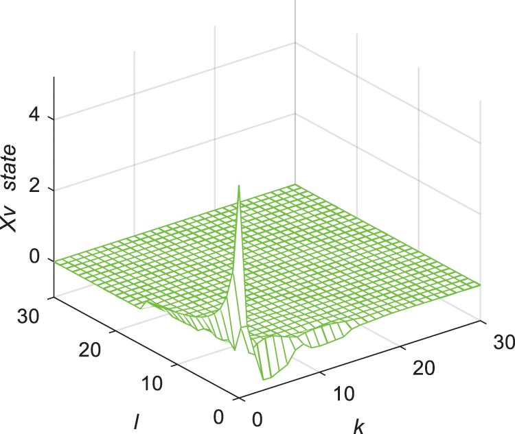
Figure 2: Response of state $xv(k,l)$

images

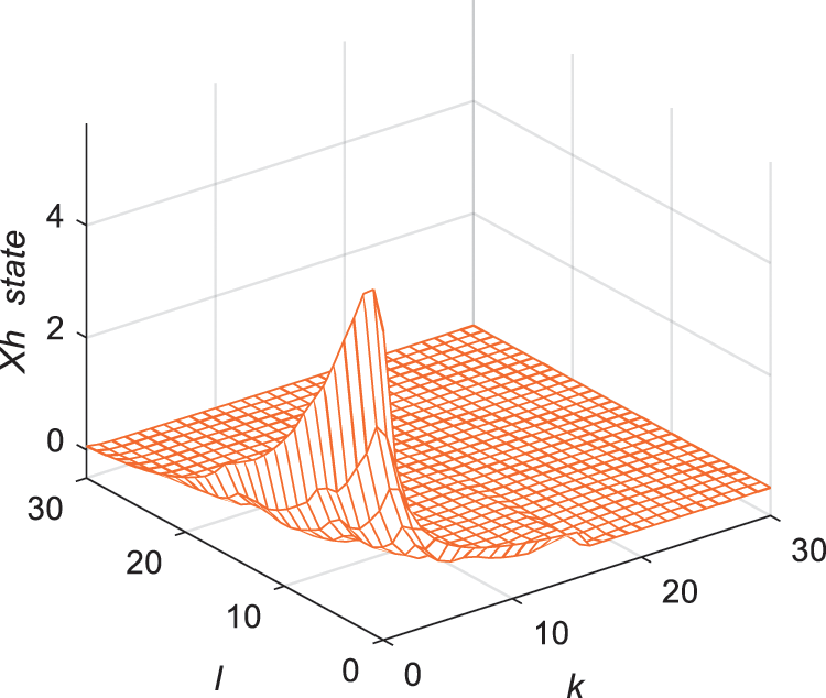
Figure 3: Response of state $xh(k,l)$

images

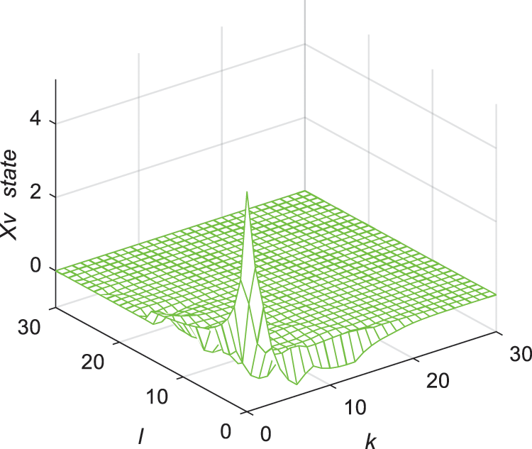
Figure 4: Response of state $xv(k,l)$

images

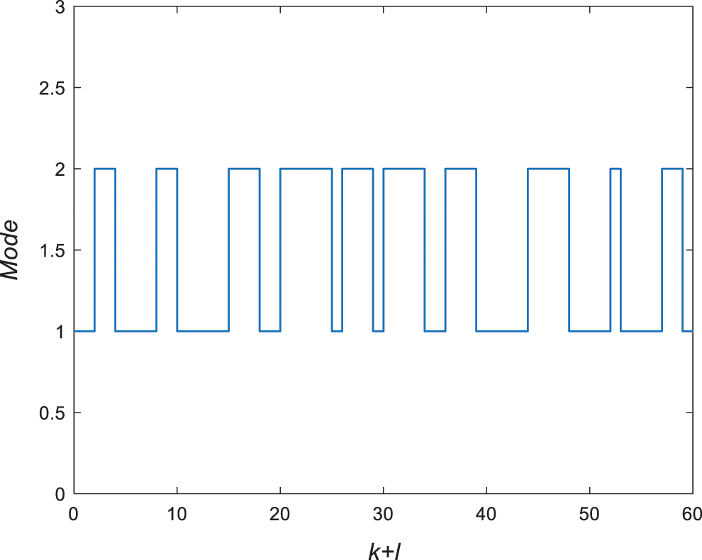
Figure 5: Switching signal

8 Conclusions

This paper has investigated the problems of stability and weighted robust $H∞$ disturbance attenuation performance analyses for 2D discrete switched systems described by the Roesser model with uncertainties. An exponential stability criterion is obtained via the average dwell time method. Some sufficient conditions for the existence of weighted robust $H∞$ disturbance attenuation level $γ$ for the considered system are derived from LMIs. Besides, a 2D output feedback controller is designed to solve the robust $H∞$ control problem. Finally, an example is also given to illustrate the applicability of the proposed results. The future work will be associated with the following directions: 1) stability analysis and stabilization for nonlinear continuous-time descriptor semi-Markov jump systems; and 2) finite-time stabilization for nonlinear discrete-time singular Markov jump systems with piecewise-constant transition probabilities subjected to average dwell time.

Data Availability: The authors declare that they have no conflicts of interest to report regarding the present study.

Funding Statement: Research supported by the Science and Technology Development Program of Jilin Province, the project named: Research on Key Technologies of Intelligent Virtual Interactive 3D Display System (20180201090GX).

Conflicts of Interest: The authors declared no potential conflicts of interest with respect to the research, authorship, and/or publication of this article.

References

1. I. V. Medvedeva and A. P. Zhzbko, “Synthesis of Razumikhin and Lyapunov-Krasovskii approaches to stability analysis of time-delay systems,” Automatica, vol. 51, no. 1, pp. 372–377, 2015. [Google Scholar]

2. F. Z. Taousser, M. Defoort, M. Djemai and S. Nicaise, “Stability analysis of switched linear systems on non-uniform time domain with unstable subsystems,” IFAC, vol. 50, no. 1, pp. 14873–14878, 2017. [Google Scholar]

3. Q. Zou, L. Wang, J. Liu and Y. Jiang, “A progressive output strategy for real-time feedback control systems,” Intelligent Automation & Soft Computing, vol. 26, no. 3, pp. 631–639, 2020. [Google Scholar]

4. C. Du and L. Xie, “H∞ control and filtering of two-dimensional Systems,” Application in 2-D system and definition of H∞ performance index, 1st ed., vol. 1. Berlin Heidelberg New York: Springer-Verlag, 1–12, 2002. [Google Scholar]

5. B. Lu, F. Liu, X. Ge and Z. Li, “Cryptanalysis and improvement of a chaotic map-control-based and the plain image-related cryptosystem,” Computers, Materials & Continua, vol. 61, no. 2, pp. 687–699, 2019. [Google Scholar]

6. B. Nagaraj, D. Pelusi and J. I. Chen, “Special section on emerging challenges in computational intelligence for signal processing applications,” Intelligent Automation & Soft Computing, vol. 26, no. 4, pp. 737–739, 2020. [Google Scholar]

7. F. Xia and S. Huang, “Application research of color design and collocation in image processing,” Computer Systems Science and Engineering, vol. 35, no. 2, pp. 91–98, 2020. [Google Scholar]

8. R. N. Yang, L. L. Li and X. J. Sun, “Finite-region dissipative dynamic output feedback control for 2-D FM systems with missing measurements,” Information Sciences, vol. 514, no. 9, pp. 1–14, 2020. [Google Scholar]

9. H. Trinh and L. V. Hien, “Prediction-based approach to stabilization of 2-D continuous-time Roesser systems with directional input delays,” Journal of the Franklin Institute, vol. 357, no. 8, pp. 4779–4794, 2020. [Google Scholar]

10. C. Sreekumar and V. Agarwal, “A hybrid control algorithm for voltage regulation in DC-DC boost converter,” IEEE Transactions on Industrial Electronics, vol. 55, no. 6, pp. 2530–2538, 2008. [Google Scholar]

11. L. V. Hien and H. Trinh, “Switching design for suboptimal guaranteed cost control of 2-D nonlinear switched systems in the Roesser model,” Nonlinear Analysis: Hybrid Systems, vol. 24, no. 1, pp. 45–57, 2017. [Google Scholar]

12. L. Li, X. Li and S. Ye, “Dynamic output feedback H∞ control for 2D fuzzy systems,” ISA Transactions, vol. 95, no. 2, pp. 1–10, 2019. [Google Scholar]

13. J. Wang, J. Liang and A. M. Dobaie, “Stability analysis and synthesis for switched Takagi-Sugeno fuzzy positive systems described by the Roesser model,” Fuzzy Sets and Systems, vol. 371, no. 1, pp. 25–39, 2019. [Google Scholar]

14. G. Ravikanth, V. K. and B. E. Reddy, “Location related signals with satellite image fusion method using visual image integration method,” Computer Systems Science and Engineering, vol. 35, no. 5, pp. 385–393, 2020. [Google Scholar]

15. S. Li and H. Lin, “On l1 stability of switched positive singular systems with time-varying delay,” International Journal of Robust and Nonlinear Control, vol. 27, no. 16, pp. 2798–2812, 2017. [Google Scholar]

16. X. Zhao, L. Zhang and P. Shi, “Stability of a class of switched positive linear time-delay systems,” International Journal of Robust and Nonlinear Control, vol. 23, no. 5, pp. 578–589, 2013. [Google Scholar]

17. R. Yang and W. Zheng, “H∞ filtering for discrete-time 2-D switched systems: An extended average dwell time approach,” Automatica, vol. 98, no. 7, pp. 302–313, 2018. [Google Scholar]

18. M. Rehan, M. Tufail and M. T. Akhtar, “On elimination of overflow oscillations in linear time-varying 2-D digital filters represented by a Roesser model,” Signal Processing, vol. 127, no. 11, pp. 247–252, 2016. [Google Scholar]

19. D. Ding, H. Wang and X. Li, “H-/H∞ fault detection observer design for two-dimensional Roesser systems,” Systems & Control Letters, vol. 82, no. 1, pp. 115–120, 2015. [Google Scholar]

20. X. Li and H. Gao, “Robust finite frequency H∞ filtering for uncertain 2-D Roesser systems,” Automatica, vol. 48, no. 6, pp. 1163–1170, 2012. [Google Scholar]

21. L. Zhang and P. Shi, “Stability, l2-gain and asynchronous H∞ control of discrete-time switched systems with average dwell time,” IEEE Transactions on Automatic Control, vol. 54, no. 9, pp. 2192–2199, 2009. [Google Scholar]

22. J. Tao, Z. Wu and Y. Wu, “Filtering of two-dimensional periodic Roesser Systems Subject to dissipativity,” Information Sciences, vol. 461, no. 12, pp. 364–373, 2018. [Google Scholar]

23. J. Lu, Z. She, S. S. Ge and X. Jiang, “Stability analysis of discrete-time switched systems via Multi-step multiple Lyapunov-like functions,” Nonlinear Analysis: Hybrid Systems, vol. 27, no. 4, pp. 44–61, 2018. [Google Scholar]

24. A. Benzaouia, A. Hmamed, F. Tadeo and A. E. Hajjaji, “Stabilization of discrete 2D time switching systems by state feedback control,” International Journal of Systems Science, vol. 42, no. 3, pp. 479–487, 2011. [Google Scholar]

25. Z. Xiang and S. Huang, “Stability analysis and stabilization of discrete-time 2D switched systems,” Circuits, Systems, and Signal Processing, vol. 32, no. 1, pp. 401–414, 2013. [Google Scholar]

26. G. Zhai, B. Hu, K. Yasuda and A. N. Michel, “Disturbance attenuation properties of time-controlled switched systems,” Journal of the Franklin Institute, vol. 338, no. 7, pp. 765–779, 2001. [Google Scholar]

27. J. P. Hespanha and A. S. Morse, “Stability of switched systems with average dwell-time,” in Proc. of the 38th IEEE Conf. on Decision and Control, Phoenix, Arizona USA, pp. 2655–2660, 1999. [Google Scholar]

28. S. P. Boyd, L. E. Ghaoui, E. Feron and V. Balakrishana, “Linear matrix inequalities in system and control theory,” Philadelphia, PA: SIAM, vol. 86, no. 12, pp. 2473–2474, 1994. [Google Scholar]

This work is licensed under a Creative Commons Attribution 4.0 International License, which permits unrestricted use, distribution, and reproduction in any medium, provided the original work is properly cited.