Computer Systems Science & Engineering DOI:10.32604/csse.2021.05468
Article

Task Allocation Approach for Minimizing Make-Span in Wireless Sensor Actor Networks

Mohammad Reza Okhovvat1, Mohammad Taghi Kheirabadi1,*, Ali Nodehi1 and Morteza Okhovvat2

1Department of Computer Engineering, Gorgan Branch, Islamic Azad University, Gorgan, Iran
2Health Management and Social Development Research Center, Golestan University of Medical Sciences, Gorgan, Iran
*Corresponding Author: Mohammad Taghi Kheirabadi. Email: m.kheirabadi@gorganiau.ac.ir
Received: 23 March 2020; Accepted: 13 July 2020

Abstract: Wireless Sensor Actor Networks (WSANs) have contributed to the development of pervasive computing wherein time consideration to perform the tasks of pervasive applications is necessary. Hence, time constraint is one of the major challenges of WSANs. In this paper, we propose an analytical approach based on queuing theory to minimize the total time taken for completion of tasks, i.e., make-span, in WSANs with hybrid architecture. The best allocation rates of tasks to actor nodes are figured out through solving inequities and qualities resulting from a steady state analysis of the proposed model. Applying the calculated tasks arrival rates at each of the actors, the make-span could be minimized. To assess the accuracy of the tasks assignment rates to each of the actors attained from the suggested analytical approach and to provide a graphical representation of the WSAN a formal model in terms of the generalized stochastic Petri net (GSPN) is presented. The proposed GSPN model is analyzed, tasks distribution weights to the actors are determined, and then tasks allocation rates can be computed. Comparing the results achieved from the analytical approach and the GSPN model demonstrates that allocation rates and hence, the make-span figured out from proposed approach and the formal model are the same. Experimental results in typical scenarios show shorter make-span and longer network lifetime compared to when one of the two popular traditional task allocation algorithms, namely, opportunistic load balancing (OLB), and stochastic allocation (SA) algorithms, is used.

Keywords: GSPN; make-span; optimization; queuing system; task allocation

1  Introduction

A group of wirelessly communicative stationary sensor nodes and actor nodes that gather environmental information and behave in reply to sensory information, respectively, build up a wireless network called Wireless Sensor Actor Network (WSAN) [1,2]. The constituent parts of WSANs can be configured differently according to the requirements of applications and existing technologies. In this context, the term actor has a different meaning as compared to the meaning of the term actuator. An actuator is an element that converts a control signal to an action, but an actor consists of one or more actuators and has the capability to perform networking-related functions such as send, receive and process data. A typical WSAN contains various nodes i.e., sensors, actors, and network sink(s). Sensors have two specific responsibilities, i.e., (a) to collect environmental information, and (b) to send that information to the network sink or directly to actors based on the network architecture. This information can be used by the sink to decide and inform actors about what they need to do. Finally, tasks are carried out by actors. In this paper, WSANs with hybrid architecture is considered [3]. However, actors are the responsible nodes to perform both global and local tasks and possibly informing the sink about the action taken, or could inform the sink and wait for additional commands. Hence, in hybrid architecture, we deal with two groups of tasks. Global tasks are complex, and usually carried out by sensors sending information through the network sink. In this case, the sink then decides on an action set, sending requests for action to a series of actors. Local tasks are simpler, fulfilled by sensors sending information direct to a specific actor, who then performs the simple task necessary. According to the importance of global tasks, they may be considered in a higher priority in the execution compared with local tasks.

One of the main challenges of WSANs is to efficiently use all its capabilities at its disposal to satisfy the quality as well as functional requirements of running applications. In WSANs with hybrid architecture, this challenge can be partly resolved by selecting the best actors to execute tasks using quality parameters such as make-span, reliability, and network lifetime [4–6]. In WSANs, the network sink is responsible to decide on the most appropriate set of actors to run global tasks. Moreover, local tasks should be done by the most appropriate actors which are the closest actors to the events or can be selected from the decision making processes in peer group of actors. Having decided on an operative assignment pattern, figuring out the most appropriate allocation rate to each actor is very important. The challenge is thus to find a dispatching rate to each actor that minimizes the completion time of tasks.

In this paper, we consider WSANs with hybrid architecture and attempt to minimize the total completion times of all tasks in the network, i.e., make-span. To determine the appropriate allocation rate of global tasks to actors, the sink should get an approximation of the capability of each actor first to calculate a proper allocation rate for that actor accordingly. However, minimizing make-span is mainly important to critical applications of WSANs wherein delays may result in disasters [7,8].

The rest of paper is organized as follows: Notable related works are presented in Section 2. Section 3 described our assumptions. In Section 4, our proposed approach is presented. Section 5 presents the proposed GSPN model. Section 6 presents the experimental results, and Section 7 concludes the paper and presents future works.

2  Related Work

There are various research works on scheduling modeling and analysis of wireless sensor actor networks.

Okhovvat et al. [7] proposed a time and energy aware approach to assign tasks to actors in WSANs. They first calculate the ability of each actor to carry out tasks and then use this information to assign tasks to actors in such a way to reduce the network make-span. They reported 45% amelioration in network make-span compared to when they apply the opportunistic load-balancing algorithm. Although they have provided an appropriate tradeoff between make-span and load balancing, the limitation on the size of queue of each actor has been ignored.

de Farias et al. [9] proposed a task scheduling algorithm for WSANs to mend the energy efficiency and so, enlarging the network lifetime. To reach this goal, their algorithm tries to utilize the characteristics of applications with typical tasks and avoid repeating tasks unnecessarily. However, their approach can increase the total remaining energies of actuators, but neither make-span nor reliability of services has been considered by their algorithm.

Sharifi and Okhovvat [10] have proposed a scalable task scheduling algorithm in WSANs with semi-automated architecture, called Scate. The dual objective of Scate is to reduce the make-span and increase the residual energy of actors. To allocate tasks, when the number of large tasks is less than the number of small tasks, Scate allocates smaller tasks to the fastest actors. Otherwise, it allocates larger tasks to the fastest actors. Scate assumes that tasks are independent, so the probable dependencies between tasks are not considered. The main drawback of their algorithm is that it does not guarantee the execution deadline for applications.

Shu et al. [11] presented an energy aware scheduling algorithm to increase the network lifetime while making strict sensing guarantees in the WSN. In order to verify their algorithm, extensive assessments of its performance via simulations were performed and about 39.2% improvement of network lifetime over the baseline method was reported. The main drawback of their algorithm is that neither the reliability of services nor the execution deadline for applications was considered in their work.

Yang and Lee [12] proposed a fault-tolerant allocation technique to tolerate failures in more than one actuator. Their method is based on the redundancy wherein the redundant actuators are redistributed to handle failures. Their method does not consider time as an important parameter in sensor and actuator networks.

Okhovvat et al. [13] proposed a scheduling solution to reduce the total completion time of a WSAN. Their solution is based on queuing theory and only can be applied to WSANs with half-automated architecture [10] and hence, it is not usually applicable to real applications which are typically compatible with hybrid architecture.

All the above research works try to model and evaluate task scheduling in WSANs while many of them do not consider both local and global tasks since they match one of the semi-automated or full automated architecture. However, considering hybrid architecture and applying GSPN models, it is possible to model both simple and complicated task execution within WSAN and evaluate the utilization of actor nodes in a WSAN.

3  Assumptions

We have considered a WSAN with hybrid architecture comprising a singleton sink and m actors Aj (j ∈ {1, …, m}) wherein actors have to perform n tasks Ti (i ∈ {1, … , n}). In such a network, a schedule for each task is an allocation of one or more time slots to one or more actors [10,11]. In this paper, we have compelled the objective of our approach to lessen the completion time of tasks assigned to each actor in order to reduce the make-span. This is achieved by calculating the ability of each actor at the time of assignment of tasks, such as its current task load and its speed, in performing tasks.

We have further assumed that tasks are independent and non-preemptive and the generation rate of tasks follows a Poisson distribution.

4  Proposed Approach

We compute the make-span as the sum of the completion time of assigned tasks to each actor. Every actors is modeled by a M/M/1 queuing system [14,15] wherein local tasks and global tasks arrive at actor Ai with λ'i and λi rate and are done with µi rate. Fig. 1 illustrates the queuing model of such a network. To reduce the make-span, we should adjust the distribution rate of tasks to actors appropriately.

To carry out steady state analysis on the actors, the sum of the local and global tasks arrival rates in each of the actors have to be less than the corresponding actor’s service time. Thus, (1) must be satisfied for all of the actors.

0≤λi+λi′<μi,∀i;1≤i≤n (1)

In our supposed model, global tasks are generated by the sink, but local tasks are determined by actors. Both local and global tasks are generated according to the sensory information where global tasks and local are determined and allocated to the appropriate actors, respectively. It is assumed that the generation of global tasks and also local tasks follows a Poisson process with λ and λ’ rates, respectively. Based on the splitting Poisson process [16], global tasks are dispatched to selected actors with λi rate defined as follows for n actors:

λ=∑i=1nλi (2)

Figure 1: Queuing network model for a WSAN

Similarly, local tasks are mapped to appropriate actors with λi′ rate defined as follows for n actors:

λ′=∑i=1nλi′ (3)

As the key goal of the presented approach is to minimize the network make-span, the distribution rate of tasks to all actors should be estimated appropriately. In other words, our approach aims to find allocation rates λ’i and λi(i ∈ {1, … , n}) to minimize the completion time of tasks allocated to the actors. Since the interval time between the allocations of two sequential tasks in actor Ai and the service times of the actors follow an exponential distribution, we assumed each actor as a M/M/1 queue. Considering Eq. (1) for each actor Ai, the queuing system that matches each actor is stable, making the steady state analysis possible for each actor. Fig. 2 shows the continuous time Markov chain (CTMC) model of actor Ai as a M/M/1 queue.

Figure 2: CTMC for an actor Ai

In Fig. 2, each ellipse denotes a state of actor Ai, and the related numbers inside each ellipse show the number of existing local and global tasks in the queue of actor Ai shown with i and j, respectively. To get a steady state analysis of CTMC shown in Fig. 2, we use following relations where πi denotes the steady state probability of existing tasks in state i.

(λi+λi′)π0,0=μiπ1,0+μiπ0,1 (4)

The total probability given by Eq. (5) is always equal to 1 and local and global tasks arrive to each actor according to independent Poisson processes with rate λi and λi′ , respectively.

∑i=0nπi=1 (5)

The service times of all tasks are exponentially distributed with the same mean 1 /μi . We assume that

ρi+ρi′<1 (6)

where ρi = λi/μi and ρi′ = λi′/μi i.e., the occupation rate due to global tasks and local tasks, respectively. We assume that tasks are non-preemptive and global tasks have higher priority compare with local tasks.

From equality system Eqs. (4) and (5), the mean response time or make-span for global tasks, Ti, can be calculated by Eq. (7):

Ti=Ni/µi+1/µi+ρi′ρi′/µi (7)

where N represents the mean number of global tasks assigned to the actor i. Eq. (7) shows that if an arriving global task finds a local task in service, it cannot start as long as the local task is in service. According to the Little theorem [16], we get Eq. (8) wherein N denotes mean number of global tasks waiting to be run by the actor i and λi shows the arrival rate of global tasks to the actor i:

Ni=λi⋅T (8)

by applying Eqs. (7) and (8), we deduce Eqs. (9) and (10):

Ti=(1+ρi′)/μi1−ρi (9)

Ni=(1+ρi′)ρi1−ρi (10)

Similarly, we can calculate mean number of waiting local tasks, N’, by Eq. (11):

Ni′=(1−ρi(1−ρi−ρi′))ρi′(1−ρi)(1−(ρi+ρi′)) (11)

By using little theorem, mean completion time of local tasks can be computed:

Ti′=(1−ρi(1−ρi−ρi′))/μi(1−ρi)(1−(ρi+ρi′)) (12)

To calculate the total completion time of tasks that should be performed by actors in the WSAN, we apply Eq. (13) to compute the completion time of tasks in each actor:

TiTotal=Ti′+Ti (13)

The make-span of the WSAN is defined as the maximum completion times of all the actors. Eq. (14) shows the total make-span of the WSAN:

Make-span=Max(TiTotal),0<i≤m (14)

Finally, the main goal of this paper can be calculated by Eq. (15).

Goal:

Min{Max[(T1′+T1),(T2′+T2),…,(Tm′+Tm)]} (15)

However, the resulted inequality and equality system could be answered using methods existing in nonlinear programming [17]. It should be noted that the details of the approach are ignored considering the fact that the mathematical methods to solve these systems are very common and can be found in various references such as [17]. We used the GAMS software [18] to solve the problem. Therefore, the tasks arrival rates at each of the actors was figured out. Then, applying the resultant tasks allocation rates to each of the actors, the make-span could be minimized.

5  The Proposed Model

One of the popular graphical tools used for formal description of a system is Petri Net (PN) [19,20]. This tool in its various shapes and types and can be used to study distributed environments in which dynamics are specified by synchronization, concurrency and mutual exclusion and conflicts [21,22]. PNs can be used to verify the system invariants like boundedness, liveness and so on. Typically, a PN can be defined as follow:

Definition 1. A typical PN is a 5-tuple PN = (P, O, I, T, M0) with P ∩ T = Ø wherein the elements of the tuple represent

•   Finite set of places P = {P1, P2, …, Pn}; P ≠ Ø,

•   Finite set of output arcs O ⊂ T x P; O ≠ Ø,

•   Finite set of input arcs I ⊂ P x T; I ≠ Ø,

•   Finite set of transitions T = {Tl, T2, …, Tn}; T ≠ Ø ,

•   Finite set of initial marking M0 = {m01, m02, …, m0m}; M0 ≠ Ø.

A PN is a directed bipartite graph wherein places are shown by circles and transitions are shown by bars or boxes. Places may hold tokens shown by black dots. The state or marking of a net is its mapping of tokens to places. If a transition fire, the tokens move from the input places of that transition to the related output places. In the basic PN models, no priority between transitions is seen and the transitions fires non-deterministically. In means that without defining an execution policy, the execution of Petri nets is non-deterministic and if more than one transition is enabled at the same time, any one of them may fire. However, various extensions of PNs have been presented so far to evaluate system behaviors. To study a system, one of the most important aspects is to evaluate the system behavior in the periods of time. In PN models, time usually associates to the transitions, timed-transition petri net (TTPNs), or to the places, timed-place petri nets (TPPNs). The both TTPN and TPPN models are also categorized further based on whether the times mentioned are stochastic or deterministic. If the time is stochastic, the class of such PNs is named as stochastic Petri nets (SPNs). If the time is deterministic, the class of such PNs is called timed Petri nets (TPNs). SPNs and TPNs are categorized in TTPNs and TPPNs classes, respectively. However, SPN has been extended and a powerful extension called GSPN resulted. GSPN has two further features compared with SPN which are immediate transitions and inhibitor arcs. The role of the immediate transitions is to make some markings called vanishing markings which are not correspond to states. The role of the inhibitor arcs is just to remove some potential transitions and markings from the reachability graph. Although all of the transitions in SPNs are timed transitions there are two different types of transitions in GSPNs: timed transitions and immediate transitions. In GSPN models, an immediate transition fires in zero time wherein as in the case of SPNs, a timed transition fire in a random and exponentially distributed enabling time. Typically, a GSPN can be defined as follow:

Definition 2. A GSPN typically can be define as a 9-tuple GSPN = (P, O, I, T, M0, Timmediate, Ttimed, W) where PN = (P, O, I, T, M0) is the marked PN underlying the GSPN as described in the definition 1. The other elements of the tuple represent

•   Finite set of immediate transitions Timmediate ⊂ T; T ≠ Ø,

•   Finite set of timed transition Ttimed ⊂ T; T ≠ Ø,

•   Timmediate ∩ Ttimed = Ø , Timmediate ∪ Ttimed = T,

•   W = (W1, W2, W3,…, W|T|) is an array whose entry Wi is the parameter of the negative exponential probability distribution function of the transition firing delay when ti is a timed transition, i.e., ti ∊ Ttimed, or is a weight used for the calculation of firing probabilities of immediate transitions when ti is an immediate transition, i.e., ti ∊ Timmediate.

In the GSPN models, timed transitions and immediate transitions are generally named in the form of Tx and tx, respectively wherein x can be a mnemonic string or a number [23]. Timed transitions are shown by white rectangular boxes, but immediate transitions are drawn by bars. Through a steady state analysis of GSPN models, various performance parameters such as the probability of firing one transition, throughput and utilization of a transition, probability of being in a subset of markings and mean number of the tokens in a specific place is computed [24].

In this paper, a typical WSAN with hybrid architecture is graphically modeled by GSPNs wherein the SHARPE package [25] is used to model and analyze the proposed GSPN. Then, by determining the proper tasks allocation rate at each of the actors, the make-span is estimated and minimized. Fig. 3 demonstrates the GSPN model of the WSAN task assignment model showed in Fig. 1. In this model, the black bars denote immediate transitions and the rectangles denote timed transitions. The arrival and execution of each task is represented by two separate timed transitions associated with exponential distributed firing time. Tasks transmitted to the actors are denoted by immediate transitions that each of them has a specific firing weight. These weights denote the firing probabilities of the immediate transitions.

The priority of each global task toward a local task is showed by an inhibitor arc. The circles represent places and they can have tokens. Tokens in this model can denote either global tasks or local tasks. Queues of each actor also are denoted by places. In order to compute the make-span of the GSPN model, we need to get the busy time of the actors in steady state of the system. The SHARP is able to compute the steady state probability that a particular place is full. Hence, we can figure out the busy times of actors shown with places in the GSPN. Tuning the allocation weights of the immediate transitions tGi, to minimize the maximum value of the places representing the buffers of actors PAi, the best allocation weights are determined. If the calculated allocation weights multiply by the global tasks generating rate at the sink, the most appropriate allocation rates at each of the actors can be approximated. Using the figured out distribution rates of tasks to each actor, the minimum make-span is resulted. The meanings of the transitions and places in Fig. 3 are as follows:

•   Transitions

TSink: models the generating rate of global tasks by the sink at rate λt

TLQi: models the arrival of local tasks at rate λ'i

TAi: models the execution of tasks in the actor i with rate λ'i

tGi: models the process of allocating tasks done by the sink

t'Pi: models the choice of the local tasks to be done by the actor i

tpi: models the choice of global tasks to be done by the actor i

•   Places

PSink: models the queue of the sink.

PLQi: models the queue of local tasks in the actor i.

PGQi: models the queue of the global tasks in the actor i.

PAi: models the task execution restrictions in the actor i. Only a single token can be placed in the place PAi at each time.

Figure 3: Proposed GSPN model for a WSAN task allocation

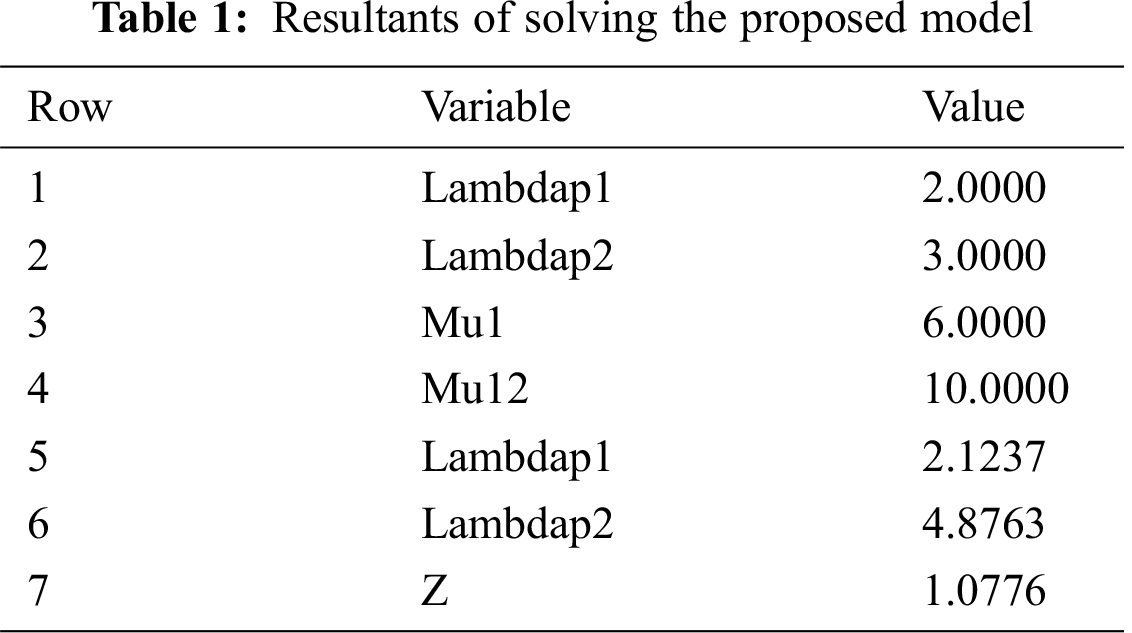
As a simple example, we assume a WSAN including two heterogeneous actors, A1, A2. These actors have the same communication bandwidth on their links, but their throughputs are different (µ1 = 6, µ2 = 10). It is assumed that the average generation rate of global tasks by the sink is λt = 7 tasks per second. It is also supposed that the mean generation rate of local tasks by the actors A1, A2 are λ'1 = 2 and λ'2 = 3 tasks per seconds, respectively. Since sensory information of a local task related to an event is directly transmitted to the closest actor, we can just adjust the assignment rate of global tasks to the actors. Hence, the goal is to determine the best rate of allocation of global tasks to actors through a steady state analysis of the proposed model. Applying Eq. (15) to the assumed WSAN, relation Eq. (16) is resulted. Results achieved from solving Eq. (16) are recorded in Tab. 1.

Goal:

Min{Max[(36−λ1(4−λ1)6(6−λ1)(4−λ1)+43(6−λ1)),(100−λ2(7−λ2)10(10−λ2)(7−λ2)+1.310−λ2)]} (16)

As shown in Tab. 1, to have minimum make-span in the example, the rates of arrival global tasks to the actors A1 and A2 should be λ1 = 2.1237 and λ2 = 4.8763, respectively. As shown in Fig. 4, the presented GSPN model of the supposed WSAN has been simulated using SHARP package. In order to minimize the make-span of the assumed WSAN, the allocation weights of the immediate transitions, tg1 and tg2, should be tune appropriately.

To find the best weights for the immediate transitions tg1 and tg2, the weight of tg1 is grown monotonically by step 0.1 from zero to one. Because of the relation Eq. (17), the weight of tg2 is reduced simultaneously from 1 to 0 by the same step. Fig. 4 shows the GSPN model of the example.

tg1+tg2=1 (17)

SHARPE package provides the facility to compute the steady state probability that a definite place is full. Applying this metric to places representing actors, the period of times in which related actor is busy can be determined. According to the simulation results, the maximum value of these probabilities in PA1 and PA2 is minimized when the weight of tg1 and tg2 attain to 0.3 and 0.7, respectively. Multiplying these weights by λt, the allocation rates of global tasks to A1 and A2 are resulted (λ1 = 2.1, λ2= 4.9). Finally, adding allocation rate of global tasks and local tasks to each actor, the most suitable allocation rate of tasks at each actor will be 4.1 and 7.9 resulted which are lead to minimum make-span. However, the calculated values for λ1 and λ2 are almost the same as the ones attained by analyzing the proposed mathematical approach. However, the correctness and the accuracy of the results gotten from solving the proposed mathematical model are confirmed by the results gotten from GSPN model.

Figure 4: Proposed GSPN model of the example

To evaluate the efficiency of the proposed approach, a more general and thorough evaluation should be performed, which is the subject of the next section.

6  Experimental Results

To illustrate the efficiency of the proposed approach, in a typical scenario, the approach is compared to stochastic allocation (SA) and opportunistic load balancing (OLB) algorithms in terms of make-span and network lifetime. Moreover, to assess the effect of scale on the efficiency of the approach, we executed simulations in both small and large scales using two different settings. In the small scale, we considered a 2D space, square field, 10m × 10m, containing100 sensor nodes with 1 meter transmission range, and 7 actor nodes. We have assumed that the tasks to be executed by actors were independent and that actors could browse the whole network with no constraints on routing hops. In the large scale, we considered a 2D space, square field, 100 m × 100 m containing 10000 sensors with 1 meters transmission range, and 20 actor nodes. In both scenarios, it is assumed that sensory information of a local task is transmitted to the closest actor directly and then, after determining the proper task (local task) by the actor, the task is done by that actor. The sensory information of global tasks is sent to the sink and the sink determines the right actions to be taken by the actors and assigns these actions (global tasks) to proper actors. Since the sink is usually faster than actors and it has less faults (or ideally has no faults at all), we have supposed that the queue of the sink never overloads. The size of a queue at each actor was supposed to be 10 and to simplify we assumed that the sizes of all tasks were the same. Actors were chosen from three different categories with slow, medium and fast service rates. As Figs. 5 and 6 show, the presented approach results in the best make-span in both small scale and large scale; thereafter, OLB results in better make-span in both scales.

Figure 5: Make-span in small scale network

To have better evaluations, we also compared our approach in terms of network lifetime. The network lifetime is evaluated in terms of all of the actor nodes alive (ANA) and half of the actor nodes alive (HNA) for the sake of clarity. As shown in Fig. 7, in terms of ANA our approach has done considerably better in both small and large scales. In the small scale wherein the required time to transmit data between sink and actors is not much compared to the execution time of tasks on the actors, our approach and OLB have nearly similar behavior (Fig. 8) in terms of network lifetime, but it operates considerably better than SA algorithm. All in all, experimental results demonstrate that our proposed approach is the best in extending the network lifetime in both small and large scale settings compare to OLB and SA algorithms, while SA results in the worst network lifetime (Figs. 7 and 8).

Figure 6: Make-span in large scale network

Load balancing is the capital goal of OLB attained by keeping all actors as busy as possible [26]. This algorithm allocates the tasks based on minimum estimated finish time of tasks in arbitrary order. SA algorithm assigns tasks to actors arbitrary and therefore, several tasks may be allocated to some actors while other actors are idle. This will unbalance the energy consumption of the actors and is lead to network partitioning. Thus, as we expected, the SA algorithm results in the worst ANA and HNA in compare with the two other approaches. However, our proposed approach allocates tasks to actors based on their capability to minimize the make-span and implicitly improves the balanced loads on the actors. That is why the experimental results illustrate that our proposed approach can improve the network lifetime in both small and large scales better than the OLB and SA algorithms.

Figure 7: Network lifetime in terms of ANA

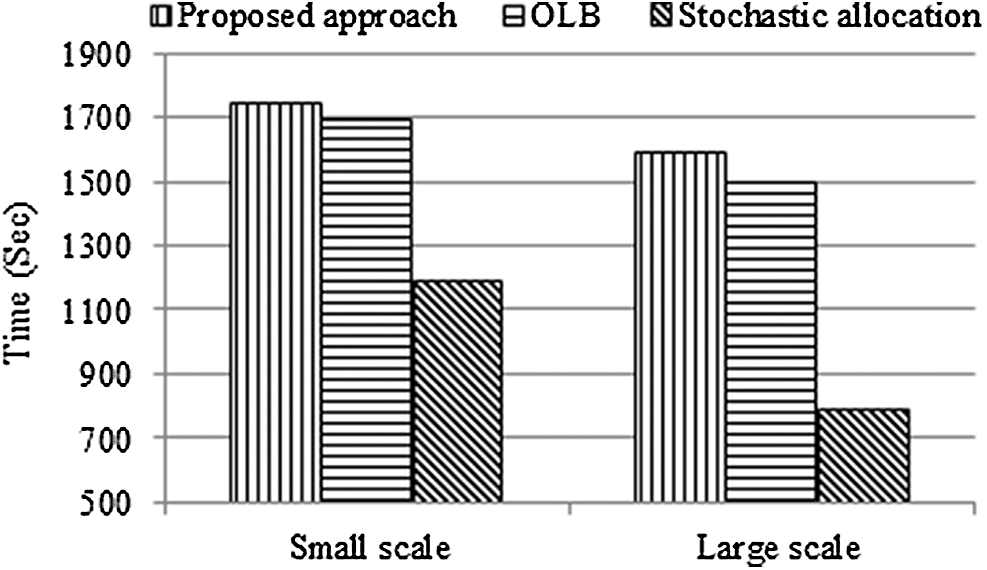
Figure 8: Network lifetime in terms of HNA

7  Conclusion and Future Works

We proposed an analytical approach to reduce the make-span of WSANs in which queuing theory was used to model the network. In the proposed approach, the most appropriate allocation rate of global tasks to each actor is determined by the sink. To achieve this goal, steady state analysis is applied to the proposed model and equalities and inequalities should be solved. Using the arrival rate of tasks to each actor, the completion time of tasks to be performed is minimized. Results of experiments on typical scenarios in small and large scales show the superiority of our proposed approach in terms of reducing make-span and enlarging network lifetime compare to two traditional task allocation algorithms, namely, the OLB, and SA algorithms.

Consideration of multi-objectives (e.g., enhancing remaining energy and reducing make-span), task deadlines in support of real-time applications, limitation of tasks queues capacity, and scalability of the network are the open issues of the approach.

Acknowledgement: The authors want to express their gratitude to the reviewers for their careful and meticulous reading of the paper.

Funding Statement: The authors received no specific funding for this study.

Conflicts of Interest: The authors declare that they have no conflicts of interest to report regarding the present study.

References

 1.  J. Shi, M. Sha and Z. Yang, “Distributed graph routing and scheduling for industrial wireless sensor-actuator networks,” IEEE/ACM Transactions on Networking, vol. 27, no. 4, pp. 1669–1682, 2019. [Google Scholar]

 2.  L. Jóźwiak, “Advanced mobile and wearable systems,” Microprocessors and Microsystems, vol. 50, pp. 202–221, 2017. [Google Scholar]

 3.  M. Sharifi and A.Najari Alamuti, “A hybrid physical architecture for coordination in wireless sensor and actor networks,” International Review on Computers and Software (IRECOS), vol. 2, no. 5, pp. 555–560, 2007. [Google Scholar]

 4.  T. Mylvaganam and M. Sassano, “Autonomous collision avoidance for wheeled mobile robots using a differential game approach,” European Journal of Control, vol. 40, no. 2, pp. 53–61, 2018. [Google Scholar]

 5.  T. Rashid, D. Y. Zhang and D. Wang, “SocialCar: A task allocation framework for social media driven vehicular network sensing systems,” in 15th Int. Conf. on Mobile Ad-Hoc and Sensor Networks (MSNShenzhen, pp. 125–130, 2019. [Google Scholar]

 6.  J. Chen, X. Cao, P. Cheng, Y. Xiao and Y. Sun, “Distributed collaborative control for industrial automation with wireless sensor and actuator networks,” IEEE Transaction on Industrial Electronics, vol. 57, no. 12, pp. 4219–4230, 2010. [Google Scholar]

 7.  M. Okhovvat and M. R. Kangavari, “TSLBS: A time-sensitive and load balanced scheduling approach to wireless sensor actor networks,” Computer Systems, Science and Engineering, vol. 34, no. 1, pp. 13–21, 2019. [Google Scholar]

 8.  J. Yang, H. Z. Li, W. Li and X. B. Liu, “Research on task allocation of geographic location related mobile sensing system,” Journal of Information Hiding and Multimedia Signal Processing, vol. 8, no. 1, pp. 19–30, 2017. [Google Scholar]

 9.  C. M. de Farias, L. Pirmez, F. C. Delicato, W. Li, A. Y. Zomaya et al., “A scheduling algorithm for shared sensor and actuator networks,” in Int. Conf. on Information Networking (ICOINBangkok, pp. 648–653, 2013. [Google Scholar]

10. M. Sharifi and M. Okhovvat, “Scate: A scalable time and energy aware actor task allocation algorithm in wireless sensor and actor networks,” ETRI Journal, vol. 34, no. 3, pp. 330–340, 2012. [Google Scholar]

11. Y. Shu, K. G. Shin, J. Chen and Y. Sun, “Joint energy replenishment and operation scheduling in wireless rechargeable sensor networks,” IEEE Transaction on Industry Informatics, vol. 13, no. 1, pp. 125–133, 2017. [Google Scholar]

12. I. Yang and D. Lee, “Networked fault-tolerant control allocation for multiple actuator failures,” Mathematical Problems in Engineering, vol. 2015, no. 14, pp. 1–14, 2015. [Google Scholar]

13. M. Okhovvat, M. R. Kangavari and H. Zarrabi, “An analytical task assignment model in wireless sensor actor networks,” in IEEE 7th Int. Conf. on Consumer Electronics—Berlin (ICCE-BerlinBerlin, pp. 195–199, 2017. [Google Scholar]

14. M. Moshtagh, J. Fathali and M. Smith, “The stochastic queue core problem, evacuation networks, and state-dependent queues,” European Journal of Operational Research, vol. 269, no. 2, pp. 730–748, 2018. [Google Scholar]

15. J. Kim, A. Dudin, S. Dudin and C. Kim, “Analysis of a semi-open queuing network with Markovian arrival process,” Performance Evaluation, vol. 120, pp. 1–19, 2018. [Google Scholar]

16. K. S. Trivedi, “Probability and statistics with reliability, queuing, and computer science applications,” 2nd ed., Wiley, USA, 2001. [Google Scholar]

17. R. Horst, P. M. Pardalos and N. V. Thoai, Introduction to global optimization (nonconvex optimization and its applications), 2nd ed. New York, USA: Springer, 2017. [Google Scholar]

18. GAMS 2020. [Online]. Available at: https://www.gams.com. [Google Scholar]

19. A. Vörös, D. Darvas, A. Hajdu, K. Marussy, V. Molnár, T. Bartha and I. Majzik, “Industrial applications of the PetriDotNet modeling and analysis tool,” Science of Computer Programming, vol. 157, no. 1, pp. 17–40, 2018. [Google Scholar]

20. J. I. Latorre-Biel and E. Jiménez-Macías, “Petri net models optimized for simulation, simulation modeling practice and theory,” IntechOpen, pp. 1–19, 2018. https://www.intechopen.com/books/simulation-modelling-practice-and-theory/petri-net-models-optimized-for-simulation. [Google Scholar]

21. M. E. Cambronero, H. Macià, V. Valero and L. Orozco-Barbosa, “Modeling and analysis of the 1-wire communication protocol using timed colored petri nets,” IEEE Access, vol. 6, pp. 27356–27372, 2018. [Google Scholar]

22. A. Kozak, D. DorotaFormanowicz and P. Formanowicz, “Structural analysis of a Petri net model of oxidative stress in atherosclerosis,” IET Systems Biology, vol. 12, no. 3, pp. 108–117, 2018. [Google Scholar]

23. M. A. Marsan, G. Balbo, G. Conte, S. Donatelli and G. Franceschinis, Modeling with generalized stochastic petri nets. New York, USA: John Wiley and Sons, 1995. [Google Scholar]

24. Q. Su, F. He, N. Wu and Z. Lin, “A method for construction of software protection technology application sequence based on Petri Net with inhibitor arcs,” IEEE Access, vol. 6, pp. 11988–12000, 2018. [Google Scholar]

25. R. Sahner, K. S. Trivedi and A. Puliafito, Performance and reliability analysis of computer systems—An example – based approach using the sharp software package. Cambridge, MA: Kluwer Academic, 1995. [Google Scholar]

26. D. Kashyap and J. Viradiya, “A survey of various load balancing algorithms in cloud computing,” International Journal of Science and Technology Research, vol. 3, no. 11, pp. 115–119, 2014. [Google Scholar]

This work is licensed under a Creative Commons Attribution 4.0 International License, which permits unrestricted use, distribution, and reproduction in any medium, provided the original work is properly cited.