Computer Systems Science & Engineering DOI:10.32604/csse.2021.016357
Article

Model Implementation and Analysis of a True Three-dimensional Display System

Ye Tian1,2, Yang Yang1,*, Han Yang3 and Ze Ji4

1Changchun University of Science and Technology, Changchun, 130022, China
2Tsinghua University, Beijing, 100084, China
3Academy of Military Sciences, Beijing, 100166, China
4Cardiff University, Cardiff, CF24 3AA, UK
*Corresponding Author: Yang Yang. Email: cloneyang@126.com
Received: 31 December 2020; Accepted: 11 March 2021

Abstract: To model a true three-dimensional (3D) display system, we introduced the method of voxel molding to obtain the stereoscopic imaging space of the system. For the distribution of each voxel, we proposed a four-dimensional (4D) Givone–Roessor (GR) model for state-space representation—that is, we established a local state-space model with the 3D position and one-dimensional time coordinates to describe the system. First, we extended the original elementary operation approach to a 4D condition and proposed the implementation steps of the realization matrix of the 4D GR model. Then, we described the working process of a true 3D display system, analyzed its real-time performance, introduced the fixed-point quantization model to simplify the system matrix, and derived the conditions for the global asymptotic stability of the system after quantization. Finally, we provided an example to prove the true 3D display system’s feasibility by simulation. The GR-model-representation method and its implementation steps proposed in this paper simplified the system’s mathematical expression and facilitated the microcontroller software implementation. Real-time and stability analyses can be used widely to analyze and design true 3D display systems.

Keywords: True 3D display system; method of voxel molding (MVM); Givone–Roessor (GR) model; asymptotic stability; Bounded-Input Bounded-Output (BIBO) stability; real-time display

1  Introduction

In recent years, with advances in optical and computer technology, stereoscopic display technology has undergone accelerated development. As a result, people are pursuing a more realistic display effect from the traditional two-dimensional (2D) display to three-dimensional (3D) display [1]. Among these developments, the most representative display is the true 3D display system.

For a true 3D display system, each voxel’s brightness and color should be controllable, and the relative spatial positional relationship between voxels should also be truly embodied. These goals require finding a suitable model to build a state space for the true 3D display system. Furthermore, the implementation steps and the results of performance analyses must be detailed.

In multidimensional system theory, the Givone–Roessor (GR) [2] and Fornasini-Marchesini (FM) models [3] are two widely used local state-space models. Both have been employed in the state-space modeling of multidimensional systems, including wireless sensor networks [4–8]. Compared with the FM model, the GR model can quantitatively express each dimension’s variables and then be used to analyze each dimension’s influence on the entire system. Therefore, we established a 4D GR model by introducing 3D position coordinates and one-dimensional (1D) time coordinates to model the system’s state space.

Galkowski [9] used the forward transfer operator to represent the transfer function and obtain the system implementation matrix through the matrix transformation for implementing the state-space model. The concept is simple and easily calculable. It can also be used to evaluate the influence of coefficient values on the realization matrix in implementing a multidimensional system. This flexibility, however, also can result in an infinite number of possible intermediate operations in constructing the feature matrix, making it difficult to obtain a general algorithm. Moreover, this method is not easily implemented by a computer program. Xu et al. [10] used the unit retardation factor to represent the transfer function and introduced the elementary operation approach (EOA) to give the implementation method of the system implementation matrix. In this method, however, only one order can be reduced in each supplementary operation. Although it is possible to increase the supplementary operation’s efficiency by some decomposition, only a few transfer functions can be applied to this decomposition method. The matrix method is also used to obtain a GR model with a lower order of the matrix [11], but it cannot be used to analyze the coefficient value's influence on the implementation matrix. Xiong [12] proposed an improved 3D EOA algorithm. Through matrix operation, the state-space model of the GR model can be obtained from the transfer function, and the order of the model is significantly reduced. In this paper, the EOA algorithm is extended to four dimensions and applied to the modeling and implementation steps of a true 3D display system.

When a true 3D display system works, one needs each voxel to transfer the information to the microcontroller as soon as possible for data analysis; thus, it has high real-time and stability requirements. Therefore, one must analyze the real-time functionality and stability of the GR model. Kokil [13] and Xin et al. [14] introduced 2D discrete system stability. However, if it is directly extended to multidimensional systems, many limitations still exist. Agathoklis et al. [15] introduced the bounded-input, bounded-output stability of the traditional multidimensional system, but the practical application still has many limitations. In a true 3D display system with a finite size, the voxel calculation results often must be quantified to achieve the perfect display effect. Therefore, in the present study, we introduced a quantitative model to obtain the necessary and sufficient conditions for the true 3D display system’s stability after quantization, and then provided an example to verify the model.

2  Establishment of GR Model with Method of Voxel Molding

2.1 Method of Voxel Molding

When a true 3D display system is working, a full-body cylinder-voxel space composed of several spatially discrete voxels will exist. It can be imagined that this space is a flask mold, and each voxel in the interior is sand. The sand in a sandbox has a unique 3D space coordinate and a 1D time coordinate. The 3D mathematical model of the displayed object is considered to be a mold. We assume that upon putting the mold into the sandbox, the mold will replace the sand’s space in the original sandbox and form a mold cavity. Based on this assumption, we proposed a 3D model voxel generation method—that is, the method of voxel molding (MVM).

We converted the original space’s image data to voxels according to the display’s requirements, which conform to the display unit's geometric characteristics. Then we inputted the voxels to the display unit for calibration and calculation.

In the cylinder space generated by an LED screen’s rotation, if each voxel’s coordinates generated at a certain angle (such as 3∘ ) are (x,y,z) , then the time corresponding to each voxel is t0,t1,t2,t3,...,tn .

Assuming that the 3D model from the acquisition module is stored in the form of a point cloud, the MVM steps are as follows:

1. We put the 3D model into the voxel space, and the edges of the model coincided with or approximated some voxels in the space, as shown in Fig. 1.

2. The voxel (xi,yj,zk) with the same time {t∈[t0,t1,t2,t3,...,tn]} was set as A={(xi,yj,zk,tn)} , that is, A1=(xi,yj,zk,t1) , A2=(xi,yj,zk,t2) , …, An=(xi,yj,zk,tn) .

3. We reflected the voxels’ data to the LED screen to obtain a set of 3D coordinates.

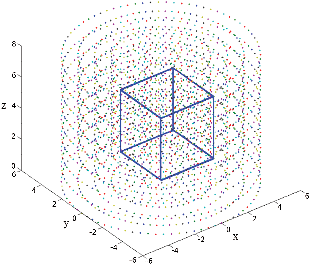
Figure 1: Schematic of 3D mold in voxel space

2.2 Establishment of GR State-space Model

The 3D position coordinates are combined with 1D time coordinates to create a 4D GR state-space model:

[xh⁡(n1+1,n2,n3,t)xv⁡(n1,n2+1,n3,t)xl⁡(n1,n2,n3+1,t)xt⁡(n1,n2,n3,t+1)]=[A1A2A3A4A5A6A7A8A9A10A11A12A13A14A15A16][xh⁡(n1,n2,n3,t)xv⁡(n1,n2,n3,t)xl⁡(n1,n2,n3,t)xt⁡(n1,n2,n3,t)]+[B1B2B3B4]u(n1,n2,n3,t),y(n1,n2,n3,t)=Cx(n1,n2,n3,t)+Du(n1,n2,n3,t), (1)

where

x(n1,n2,n3,t)=(xhT⁡(n1,n2,n3,t),xvT⁡(n1,n2,n3,t),xlT⁡(n1,n2,n3,t),xtT⁡(n1,n2,n3,t))=(xhT⁡(n1,n2,n3,t),xvT⁡(n1,n2,n3,t),xlT⁡(n1,n2,n3,t),xtT⁡(n1,n2,n3,t)),

and n1∈Z , n2∈Z , n3∈Z , and t∈Z . The vectors xh∈Ra , xv∈Rb , xl∈Rc , and xt∈Rd are the vectors of the x-, y-, z-, and time t-axis, respectively. The input vector u∈Rp and the output vector y∈Rq , A1∈Ra×a , A2∈Ra×b , A3∈Ra×c , A4∈Ra×d , A5∈Rb×a , A6∈Rb×b , A7∈Rb×c , A8∈Rb×d , A9∈Rc×a , A10∈Rc×b , A11∈Rc×c , A12∈Rc×d , A13∈Rd×a , A14∈Rd×b , A15∈Rd×c , A16∈Rd×d , B1∈Ra×p , B2∈Rb×p , B3∈Rc×p , B4∈Rd×p , C∈Rq×(a+b+c+d) , and D∈Rq×p .

Assuming that

A=[A1A2A3A4A5A6A7A8A9A10A11A12A13A14A15A16] ,

and letting r denote the order of the matrix, then r=a+b+c+d .

B=(B1T,B2T,B3T,B4T)T . For the single input single output (SISO) system, p=q=1 ; for the multiple input multiple output system, p>1 , q>1 . The voxel causal linear process in the first octant can be expressed in this model.

Considering the voxel space of size N1×N2×N3 , the display of each voxel is a linear process. Because the 3D mathematical model must be observable and realizable, the entire voxel space display is a process of linear causality in the first octant. The state-space model can represent the causality in the first octant.

3  Implementation Steps of GR Model with EOA Transformation

We performed EOA transformation to simplify the implementation of the GR model to the supplementary and transformation operations of the multidimensional characteristic polynomial matrix. This method featured easy calculation and could be used analyze the coefficient correlations on the system implementation matrix. We proposed a 4D EOA transformation and obtained the state-space model of the GR model through matrix operation.

3.1 Elementary Transformation of Matrices

Numerous elementary transformations of matrices are needed for obtaining the state-space matrix. Several of these transformations are defined below.

Let M denote a matrix and the following four kinds of row (column) transformations for a matrix denote the elementary row (column) transformations of a matrix.

1. swaprow(M,i,j) : Exchange the elements in the ith and jth rows of matrix M .

2. addrow(M,i,j,k) : Multiply all the elements in the ith row of matrix M by k , and add them to the corresponding elements in the jth row.

3. swapcol(M,i,j) : Exchange the elements in the ith and jth columns of matrix M .

4. addcol(M,i,j,k) : Multiply all the elements in the ith column of matrix M by k , and add them to the corresponding elements in the jth column.

In addition, define augment(M)=[100M].

3.2 4D EOA Transformation

Next, we implemented the matrix transformation for the 4D GR model in the SISO case (p=q=1 ) as follows:

Let Z=diag{z1Ia,z2Ib,z3Ic,z4Id} and define

M=[xBT(CZ)T(Ir−AZ)T]=[xB1B2B3B4C1z1Ia−(A1z1)T−(A5z1)T−(A9z1)T−(A13z1)TC2z2−(A2z2)TIb−(A5z2)T−(A10z2)T−(A14z2)TC3z3−(A3z3)T−(A7z3)TIc−(A11z3)T−(A15z3)TC4z4−(A4z4)T−(A8z4)T−(A12z4)TId−(A16z4)T], (2)

M0=[x1n(z1,z2,z3,z4)d(z1,z2,z3,z4)]. (3)

As shown in Y. Xiong [12], the 4D GR model’s implementation problem is to convert M0 into matrix M by supplementing operations and elementary transformation without changing the determinant value.

The matrix M requires the following properties:

1.    The first element on the diagonal can only be x .

2.    Other elements on the diagonal can only be 1D linear polynomials about variables zk,k∈{1,2,3,4} , and the constant term can only be 1.

3.    In addition to the first line, the off-diagonal element can only be a linear monomial about variables zk,k∈{1,2,3,4} .

4.    In addition to x , the elements of the first row are constant terms.

5.    The elements of the same row can only contain the same elements zk,k∈{1,2,3,4} , and from the second row all the rows are arranged in the order z1,z2,z3,z4 .

6.    The first element x on the diagonal is just a symbol, not a variable. During transformation, the position and expression of x cannot be changed.

The specific steps of the EOA transformation are as follows:

Step 1: Let any four-dimensional polynomial with no constant term be p′(z1,z2,z3,z4) . One of the variables zk,k∈{1,2,3,4} can be decomposed into the following form:

p′(z1,z2,z3,z4)=p1(zk)+p2(z1,...,zk−1,zk+1,...,z4)+zkp3(z1,z2,z3,z4), (4)

where p1(zk) is a 1D linear polynomial containing only zk ; p2(z1,...,zk−1,zk+1,...,z4) is a 4D linear polynomial without zk . p1(zk) , p2(z1,...,zk−1,zk+1,...,z4) , and p3(z1,z2,z3,z4) do not include a constant term.

Letting d^(z1,z2,z3,z4)=d(z1,z2,z3,z4)−1 , the initial matrix M0 is

M0=[x1n(z1,z2,z3,z4)1+d^(z1,z2,z3,z4)]. (5)

Let p^=d^(z1,z2,z3,z4) , q^=d^(z1,z2,z3,z4) . According to Eq. (4), x and y are decomposed into

p^=p1+p2+z1p3 ,

q^=q1+q2+z1q3, (6)

where p1 and q1 are 1D linear monomials that contain only z1 ; p2 and q2 are 3D linear polynomials that do not contain z1 ; and p3 and q3 are 4D polynomials.

The following operations are then performed:

M1=augment(M0)=addrow(M1,3,2,−z1)=addcol(M1,3,2,p3)=addcol(M1,3,1,q3)=[x10q1+q21+p1+p2−z1q3p31]. (7)

Then, the new rows generated by each operation in p3 , q3 , and M1 are sequentially operated so that terms with z1 in M1 become linear monomials concerning z1 .

Each row in M1 performs the same operation on the variables z1 , z2 , z3 , and z4 in turn, so that the diagonal elements other than x in M1 are all 4D linear polynomials with the constant term of 1.

Step 2: Assume that the matrix M1 obtained through Step 1 is

M1=[x10a1z1+a2z2+a3z3+a4z41+b1z1+b2z2+b3z3+b4z4c1z1+c2z2+c3z3+c4z4∗#1], (8)

where * and # are both linear polynomials; ai, bi, ci, and di are all coefficients, and i = {1,2,3,4}.

Convert matrix M1 obtained in the first step to M2 so that the diagonal elements in M2 except x are 1D linear polynomials with a constant term of 1, and the non-diagonal elements except the first row are all linear monomials about the variables zk,k∈{1,2,3,4} .

Perform the following operation on M1 in Eq. (8):

M2=augment(M1)→M2=addrow(M2,4,2,−1)→M2=addcol(M2,4,1,a2z2)→M2=addcol(M2,4,2,b2z2)→M2=addcol(M2,4,3,c2z2)=[x100a1z1+a3z3+a4z41+b1z1+b3z3+b4z4c1z1+c3z3+c4z4−1∗#10a2z2b2z2c2z21]. (9)

In the same row, perform similar operations on variables z3 and z4 . Then, matrix M2 is finally obtained and the first three elements of the second row in M2 are a1z1 , 1+b1z1 , and c1z1 , respectively; the remaining elements are −1:

M2=[x10000a1z11+b1z1c1z1−1−1−1∗#1000a2z2b2z2c2z2100a3z3b3z3c3z3010a4z4b4z4c4z4001]. (10)

Step 3: Through appropriate row and column transformations, each row in M2 is arranged in the order z1 , z2 , z3 , and z4 , and all of the 1D linear polynomial elements are moved to the diagonal position. Then, the term −1 is eliminated through column transformation. Finally, matrix M3 is obtained:

M3=[x10100a1z11+b1z1c1z1b1z1b1z1b1z1∗#1###a2z2b2z2c2z21+b2z2b2z2b2z2a3z3b3z3c3z3b3z31+b3z3b3z3a4z4b4z4c4z4b4z4b4z41+b4z4], (11)

and matrices A , B , and C are derived from Eq. (11).

3.3 Example

A strict causal transfer function is expressed as follows:

H(z1,z2,z3,z4)=z1+z1z2+z1z3+z1z41+z1z2+z1z3+z2z3+z1z4, (12)

and, due to the strict causality, D=H(0,0,0,0)=0 .

The initial matrix is constructed as follows:

M0=[x1z1+z1z2+z1z3+z1z41+z1z2+z1z3+z2z3+z1z4]and (13)

transformed to give

M1=augment(M0)→M1=addrow(M1,3,2,−z1)→M1=addcol(M1,3,1,z2+z3+z4)→M2=augment(M1)→M2=addrow(M2,4,2,−z2)→M2=addcol(M2,4,2,z3)→M3=augment(M2)→M3=addrow(M3,5,2,−1)→M3=addcol(M3,5,4,−z2)→M4=augment(M3)→M4=addrow(M4,6,3,−1)→M4=addcol(M4,6,1,z3+z4)→M4=addcol(M4,6,2,z3+z4)→M5=augment(M4)→M5=addrow(M5,7,6,−1)→M5=addcol(M5,7,1,z4)→M5=addcol(M5,7,2,z4)→M5=swaprow(M5,4,5)→M5=swapcol(M5,4,5)→ .

Then,

M=[x101000z11−z100−z1−z1z2z21z20000001−z2000z30z3100z3z30z3010z4z40z4001] (14)

is obtained.

According to Eq. (2), a=1 , b=2 , c=2 , and d=1 . Therefore, the order of the realization matrix is r=6 . Then,

A=[0−10−1−1−11000000−10−1−1−1001000100000100000],B=[101000], (15)

C=[110011],D=0,

are obtained. At time t , and letting the control variables

u(n1,n2,n3)=[n1+50n2+10000], (16)

the distribution of variables in the 3D volume space at t is simulated. The results are shown in Fig. 2.

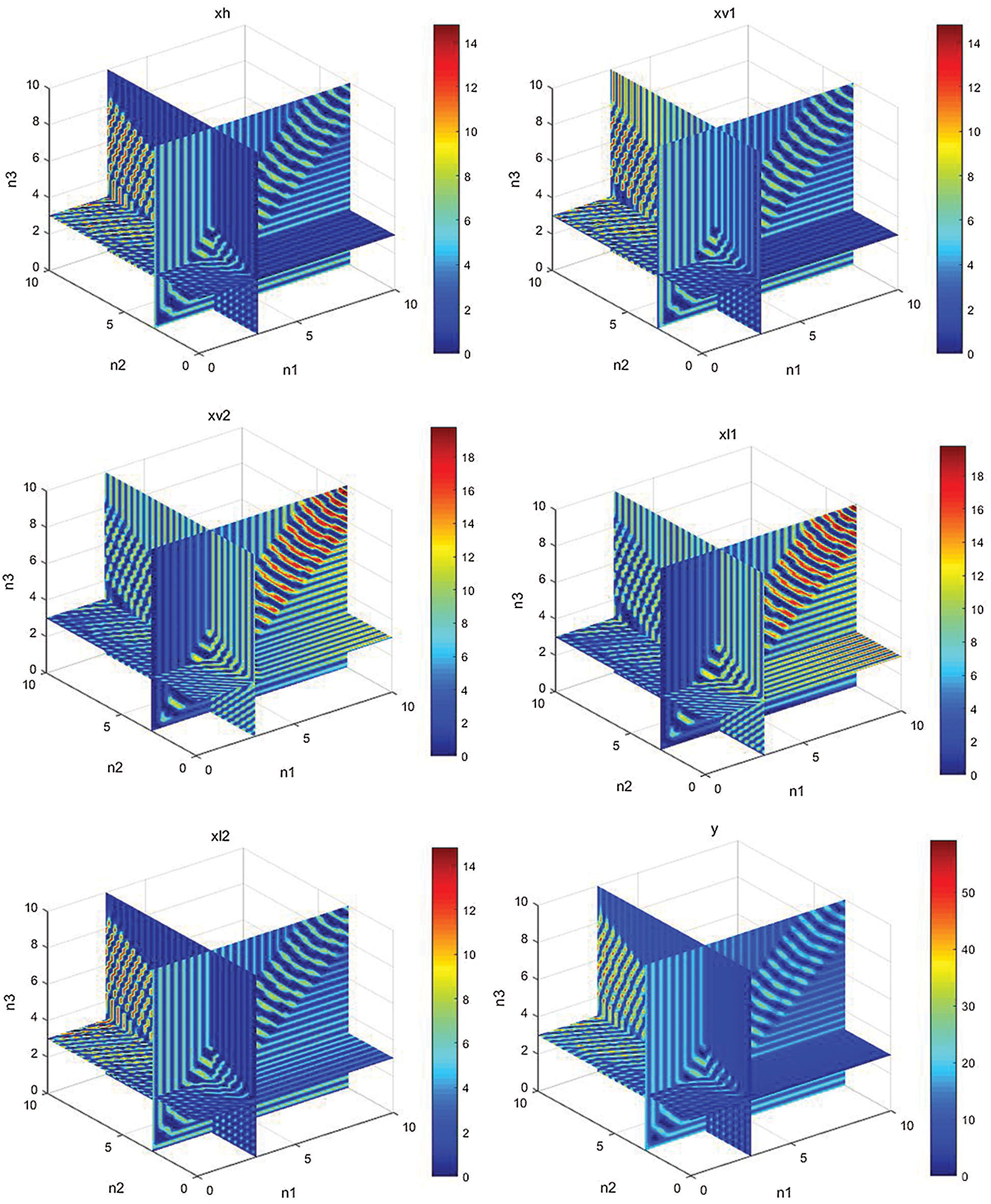
Figure 2: Simulation results in 3D space

4  Performance Analysis of GR model

We then studied the real-time performance and stability of the true 3D display system from the GR model’s state-space matrix perspective.

4.1 Real-time Analysis

4.1.1 Working Process of True 3D Display System

In the GR model, (n1,n2,n3) are the coordinates of the voxel in space, and t represents the sampling time index. x(n1,n2,n3,t) , y(n1,n2,n3,t) , and u(n1,n2,n3,t) are the state, output, and input vectors of the voxel, respectively. At time t , voxel (n1,n2,n3) sends vector xh(n1+1,n2,n3,t) to voxel (n1+1,n2,n3) , xv(n1,n2+1,n3,t) to voxel (n1,n2+1,n3) , and xl(n1,n2,n3+1,t) to voxel (n1,n2,n3+1) . Then, we calculated the output vector y(n1,n2,n3,t) .

In information processing, the problem of communication delay has always been difficult to solve [16]. For a true 3D display system with high real-time requirements and large scale, the communication between voxels will be seriously delayed, which is not conducive to the microcontroller’s data calculation and analyses. Therefore, changing the system matrix to satisfy the real-time requirements of the system is critical.

4.1.2 Implementation of Delayed Response

In model (1), if matrices A1 , A2 , A3 , A5 , A6 , A7 , A9 , A10 , and A11 are all zero, the substate vector xh(n1+1,n2,n3,t) of voxel (n1+1,n2,n3) in the x-axis direction, xv(n1,n2+1,n3,t) of voxel (n1,n2+1,n3) in the y-axis direction, and xl(n1,n2,n3+1,t) of voxel (n1,n2,n3+1) in the z-axis direction are only related to xt(n1,n2,n3,t) . Thus, it is not necessary to calculate the substate vectors for voxel (n1,n2,n3) at time t . The substate vector xt(n1,n2,n3,t+1) is used only by voxel (n1,n2,n3) , and we perform this calculation process at time t+1 . In this way, substate vectors xh(n1+1,n2,n3,t) , xv(n1,n2+1,n3,t) , and xl(n1,n2,n3+1,t) cannot be calculated at time t , and thus there is no delay in data communication. Model (1) is then changed to

[xh⁡(n1+1,n2,n3,t)xv⁡(n1,n2+1,n3,t)xl⁡(n1,n2,n3+1,t)xt⁡(n1,n2,n3,t+1)]=[000A4000A8000A12A13A14A15A16][xh⁡(n1,n2,n3,t)xv⁡(n1,n2,n3,t)xl⁡(n1,n2,n3,t)xt⁡(n1,n2,n3,t)]+[B1B2B3B4]u(n1,n2,n3,t). (17)

4.2 Stability Analysis

4.2.1 Quantitative Model

In a true 3D display system, each state component represents the gray value in a specific direction that must be controlled between (0,255). Therefore, the calculation results of each voxel must be quantized after being transmitted to the microcontroller.

Since the display system may have dimensions of different sizes, or there may be a direction that requires higher accuracy, the calculation accuracy in each direction will be different when voxels are transmitting information. In this case, the following quantitative model is adopted:

[xh(n1+1,n2,n3,t)]=Qch[[A1A2A3A4]x(n1,n2,n3,t)+[B1]U(n1,n2,n3,t)],[xv(n1,n2+1,n3,t)]=Qcv[[A5A6A7A8]x(n1,n2,n3,t)+[B2]U(n1,n2,n3,t)],[xl(n1,n2,n3+1,t)]=Qcl[[A9A10A11A12]x(n1,n2,n3,t)+[B3]U(n1,n2,n3,t)],[xt(n1+1,n2,n3,t)]=Qp[[A1A2A3A4]x(n1,n2,n3,t)+[B4]U(n1,n2,n3,t)]. (18)

In this model, Qch , Qcv , Qcl , and Qp denote the quantization operators of the x-, y-, z-, and t-axis, respectively.

4.2.2 Asymptotic Stability

In this paper, we studied the global asymptotic stability based on the 4D quantization model. Assuming that the volume space of the display system is N1×N2×N3 , then n1∈[0,N1−1] , n2∈[0,N2−1] , and n3∈[0,N3−1] . First, the following conclusion is given.

Model (18) is asymptotically stable if and only if

x(t+1)=Qp[A16x(t)] (19)

is asymptotically stable.

The detailed proof is shown in Yang et al. [17].

4.2.3 Example

The following is a concrete example of a true 3D display system. Let the GR model of a true 3D display system with a size of 4×4×4 be expressed as follows:

[xh(n1+1,n2,n3,t)xv(n1,n2+1,n3,t)xl(n1,n2,n3+1,t)xt(n1,n2,n3,t+1)]=[0000.50000.50000.50.50.50.50.375][xh(n1,n2,n3,t)xv(n1,n2,n3,t)xl(n1,n2,n3,t)xt(n1,n2,n3,t)]+[0001]U(n1,n2,n3,t), (20)

where 0≤n1≤4 , 0≤n2≤4 , 0≤n3≤4 , and U(n1,n2,n3,t)={10≤t≤50else .

As explained in Section 4.2.2, system (20) is asymptotically stable if and only if the system

x(t+1)=Qp[A16x(t)] (21)

is asymptotically stable.

The Euclidean norm of state vectors of voxels (4,4,4) and (1,1,1) are obtained by simulation, represented by p1 and p2 , respectively. The simulation results are shown in Fig. 3.

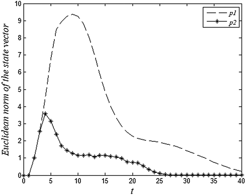
Figure 3: Euclidean norm of voxel (4,4,4) and (1,1,1) state vectors in true 3D display system of size 4×4×4

As shown in Fig. 3, after some time, the state vectors of voxels (4,4,4) and (1,1,1) tended to be 0, whereas the state vector of voxel (4,4,4) reached 0 later than that of voxel (1,1,1) . This confirmed the causality of the system in the first octant.

5  Conclusions

For the modeling and analyses of a true 3D display system, we established a 4D GR model by combining the 3D azimuth coordinates and 1D time coordinates of voxels in the imaging space. Therefore, we obtained the state-space expression of the true 3D display system. We then proposed the implementation steps with 4D EOA transformation for the GR model’s realization matrix; after describing the system working process, we analyzed the real-time and stability performance of the true 3D display system. By simplifying the system matrix, we derived the conditions for the global asymptotic stability of the system. Experimental results showed that in a true 3D display system with a size of 4×4×4 , the state vector of the voxel point converged to 0, and thus was asymptotically stable. The proposed GR-model-representation method and its implementation steps for a true 3D display system could simplify the system’s mathematical expression and facilitate microcontroller software implementation. Real-time and stability analyses can be applied widely in the analysis and design of true 3D display systems.

Acknowledgement: We thank LetPub (www.letpub.com) for its linguistic assistance during the preparation of this manuscript.

Funding Statement: This work was supported by the Key Research and Development Projects of Science and Technology Development Plan of Jilin Provincial Department of Science and Technology (20180201090gx).

Conflicts of Interest: The authors declare that they have no conflicts of interest to report regarding the present study.

References

 1.  T. Liu, “Review on research progress of true-3d volumetric display technology,” Advanced Display, vol. 10, no. 5, pp. 30–40, 2010. [Google Scholar]

 2.  R. N. Yang, W. X. Zheng and Y. R. Yu, “Event-triggered sliding mode control of discrete-time two-dimensional systems in Roesser model,” Automatica, vol. 114, no. 5, pp. 108813, 2020. [Google Scholar]

 3.  X. D. Z. Wu, “Realization method of multidimensional system and discussion of transformation between Roesser model and Fornasini-Marchesini model,” M.S. theses. Wuhan University of Science and Technology, China, 2019. [Google Scholar]

 4.  J. Yang, “Formation control and collaborative searching of swarm robotics,” Ph.D. dissertation. Harbin Institute of Technology, China, 2018. [Google Scholar]

 5.  B. Sumanasena and P. Bauer, “A Roesser model based multidimensional systems approach for grid sensor networks,” in IEEE Asilomar Conf. on Signals, Pacific Grove, CA, USA, pp. 2151–2154, 2010. [Google Scholar]

 6.  A. A. Hady, “Duty cycling centralized hierarchical routing protocol with content analysis duty cycling mechanism for wireless sensor networks,” Computer Systems Science and Engineering, vol. 35, no. 5, pp. 347–355, 2020. [Google Scholar]

 7.  M. E. Bayrakdar, “Cost effective smart system for water pollution control with underwater wireless sensor networks: a simulation study,” Computer Systems Science and Engineering, vol. 35, no. 4, pp. 283–292, 2020. [Google Scholar]

 8.  S. Kaur and V. K. Joshi, “Hybrid soft computing technique based trust evaluation protocol for wireless sensor networks,” Intelligent Automation & Soft Computing, vol. 26, no. 2, pp. 217–226, 2020. [Google Scholar]

 9.  K. Galkowski, “The state-space realization of ann-dimensional transfer function,” International Journal of Circuit Theory and Applications, vol. 9, no. 2, pp. 189–197, 1981. [Google Scholar]

10. L. Xu and S. Yan, “A new elementary operation approach to multidimensional realization and LFR uncertainty modeling: The MIMO case,” IEEE Transactions on Circuits and Systems I: Regular Papers, vol. 59, no. 3, pp. 638–651, 2012. [Google Scholar]

11. L. Xu, H. J. Fan and Z. P. Lin, “A direct-construction approach to multidimensional realization and LFR uncertainty modeling,” Multidimensional Systems and Signal Processing, vol. 19, no. 3, pp. 323–359, 2008. [Google Scholar]

12. Y. Xiong, “Multidimensional Roesser state space model based on wireless sensor networks,” M.S. theses. Wuhan University of Science and Technology, China, 2016. [Google Scholar]

13. P. Kokil, “An improved criterion for the global asymptotic stability of 2d discrete state-delayed systems with saturation nonlinearities,” Birkhauser Boston Inc, vol. 36, no. 1, pp. 2209–2222, 2017. [Google Scholar]

14. G. Xin, W. Lin, C. Fuyong, H. Li and W. Zhang, “Reliability analysis of slope stability considering temporal variations of rock mass properties,” Computers, Materials & Continua, vol. 62, no. 3, pp. 263–281, 2020. [Google Scholar]

15. P. Agathoklis and L. T. Bruton, “Practical-BIBO stability of n-dimensional discrete systems,” IEE Proceedings G (Electronic Circuits and Systems), vol. 130, no. 6, pp. 236–242, 1983. [Google Scholar]

16. B. Nagaraj, D. Pelusi and J. I. Chen, “Special section on emerging challenges in computational intelligence for signal processing applications,” Intelligent Automation & Soft Computing, vol. 26, no. 4, pp. 737–739, 2020. [Google Scholar]

17. Y. Yang, Y. Tian, Z. Liu and G. L. Chen, “Roesser model of true 3d display system and its performance analysis,” Journal of Systems Science and Mathematical Sciences, vol. 39, no. 4, pp. 534–544, 2019. [Google Scholar]

This work is licensed under a Creative Commons Attribution 4.0 International License, which permits unrestricted use, distribution, and reproduction in any medium, provided the original work is properly cited.