DOI:10.32604/csse.2021.018086
| Computer Systems Science & Engineering DOI:10.32604/csse.2021.018086 | |
| Article |
Semisupervised Encrypted Traffic Identification Based on Auxiliary Classification Generative Adversarial Network
1State Grid Jiangsu Electric Power Co., Ltd. Information and Telecommunication Branch, NanJing, 210003, China
2Institute of Information and Communication, Global Energy Interconnection Research Institute, State Grid Key Laboratory of Information and Network Security, Nanjing, 210003, China
3Engineering Research Center of Post Big Data Technology and Application of Jiangsu Province, Research and Development Center of Post Industry Technology of the State Posts Bureau (Internet of Things Technology), Broadband Wireless Communication Technology Engineering Research Center of the Ministry of Education, Nanjing University of Posts and Telecommunications, Nanjing, 210003, China
4Department of Electrical Engineering and Computer Science, Cleveland State University, Cleveland, 44115, USA
*Corresponding Author: Jiaming Mao. Email: 513222462@qq.com
Received: 24 February 2021; Accepted: 21 April 2021
Abstract: The rapidly increasing popularity of mobile devices has changed the methods with which people access various network services and increased network traffic markedly. Over the past few decades, network traffic identification has been a research hotspot in the field of network management and security monitoring. However, as more network services use encryption technology, network traffic identification faces many challenges. Although classic machine learning methods can solve many problems that cannot be solved by port- and payload-based methods, manually extract features that are frequently updated is time-consuming and labor-intensive. Deep learning has good automatic feature learning capabilities and is an ideal method for network traffic identification, particularly encrypted traffic identification; Existing recognition methods based on deep learning primarily use supervised learning methods and rely on many labeled samples. However, in real scenarios, labeled samples are often difficult to obtain. This paper adjusts the structure of the auxiliary classification generation adversarial network (ACGAN) so that it can use unlabeled samples for training, and use the wasserstein distance instead of the original cross entropy as the loss function to achieve semisupervised learning. Experimental results show that the identification accuracy of ISCX and USTC data sets using the proposed method yields markedly better performance when the number of labeled samples is small compared to that of convolutional neural network (CNN) based classifier.
Keywords: Encrypted traffic recognition; deep learning; generative adversarial network; traffic classification; semisupervised learning
Traffic classification and identification can be used to improve network management and security monitoring to improve service quality and provide a foundation for network design and planning. Network traffic identification has been studied in depth. Based on the classification methods used, network traffic identification can be divided into methods based on host attributes, payload, machine learning and deep learning. As early as 1995, scholars used traditional identification methods based on service host attributes to identify network traffic [1]. As more programs were developed to use dynamically allocated port numbers to camouflage traffic, traditional methods began to fail quickly. Academia then began to study the method of mining the flow characteristics of applications through the flow payload to classify applications [2,3]. The current identification method based on payload can manage most identification problems in nonencrypted traffic scenarios but cannot identify encrypted traffic.
With the enhancement of user security awareness and the wide application of SSL, SSH, VPN and other technologies, the proportion of encrypted traffic in network transmission is increasing. Traditional methods have been unable to accurately identify application traffic. Many scholars use machine learning to manage the problem of encrypted traffic identification. Methods based on machine learning do not need to analyze the specific structure of traffic packets, and their identification algorithms will automatically extract traffic characteristics to form a classifier [4–6]. However, the feature design of machine learning must rely on the experience of experts, and the constantly changing characteristics of encrypted traffic make this work time-consuming and labor-intensive. With increasing demand for encrypted traffic identification, the high analysis and labor costs of traditional machine learning have gradually become prohibitive.
Compared to machine learning, deep learning can better express the essential characteristics of data, which is attractive in many applications. [7,8] For example, reference Wang et al. [9] uses a data packet header and payload as input and uses convolutional neural network (CNN) and long short-term memory network (LSTM) for traffic identification. References Aceto et al. [10,11] use the first N bytes of the payload and original data; certain features in the first 20 packets before interactive communication is used as input; and the algorithm uses multilayer perceptron (MLP) for traffic identification. Reference Lopez-Martin et al. [12] combines multiple neural networks for IoT traffic identification, and reference Höchst et al. [13] uses an autoencoder (SAE) to determine web browsing interactions, game downloads, online playback uploads and other actions in network traffic. Most existing deep learning-based traffic recognition methods are based on supervised learning methods and rely on a large amount of labeled data. Conversely, unlabeled data is relatively easy to obtain. How to combine a large amount of unlabeled traffic data with a small amount of labeled traffic data to complete the classification task in a semisupervised way and alleviate the dependence of many of labeled data sets has important research significance.
To describe semisupervised learning, this paper proposes a semisupervised encrypted traffic recognition method based on the auxiliary classification generation adversarial network (SACGAN). This method implements semisupervised learning with the help of a small amount of encrypted traffic data from real applications, the data generated by the generated adversarial network (GAN), and unlabeled real traffic data. In the case of few labeled data samples, better recognition results can be obtained than supervised learning methods under the same conditions. The main contribution of this article is summarized as follows:
a) The network structure of the ACGAN is modified, and the loss function of the generator and discriminator is modified to make it possible to use unlabeled samples for semisupervised learning.
b) The improved network structure is used for encrypted traffic identification, and a semisupervised encrypted traffic identification scheme based on the ACGAN is designed.
c) Using the proposed method and the CNN classification method in the paper [14], a classification experiment was performed on the ISCX and USTC data sets. The results show that under the same conditions, the proposed method is more accurate when there are fewer labeled samples.
The organizational structure of this paper is as follows. The first chapter is an introduction, which introduces the current research status in the field of encryption traffic identification and the purpose and significance of this paper’s work. The second chapter discusses related studies and introduces the research status of the encrypted traffic identification and semisupervised encrypted traffic identification using GAN. The third chapter introduces the proposed methods, including the network structure, loss function and training method of the semisupervised auxiliary classification generating adversarial network (SACGAN). In chapter four, we introduce the proposed experiments, and perform classification experiments on ISCX and USTC data sets. Chapter five summarizes the article and proposes future research.
Since Goodfellow proposed GAN in 2014 [15], GAN has been considered a promising technology. In recent years, GAN has demonstrated advantages in image, sound, and text generation [13–20]. Due to similarities between traffic data, text and sentences, scholars consider using GAN to generate traffic data. GAN is often used to generate adversarial attack traffic to spoof detection systems [21–23]. Because data consistent with the real data distribution can be generated through antagonistic learning, GAN can also be used to balance the management of traffic data sets. The authors of reference [24] use an unsupervised learning method called auxiliary classi-fier GAN (AC-GAN) to generate comprehensive traffic samples to balance primary and secondary classes on NIMS, a well-known traffic data set that contains only SSH and non-SSH classes. Douzas et al. [25] used a conditional generation adversarial network (CGAN) to obtain the true distribution of the small sample by adding conditional in-formation to the GAN. A trained generator is then used to generate flow and perform sample balancing. However, instability and pattern collapse problems often occur in this model during training [26–28]. Similarly, Zheng et al. [29] proposed CWGAN-GP as a new oversampling method, which can learn from real data distribution based on the global information of the data set thus improving the low recognition rate of mi-nority groups in the imbalanced data set and concurrently solving the problem of mode collapse.
Currently, the semisupervised framework based on deep learning is primarily used in the fields of computer vision and natural language processing [30,31]. Existing research on semisupervised deep learning architecture is divided into two categories: (1) methods of unsupervised pretraining followed by supervised adjustment, (2) methods of unsupervised and supervised training simultaneously. Recently, Rezaei et al. [32] reduced the size of the tagged data set required to train deep learning classifiers using a semisupervised learning approach based on the concept of transfer learning. They pretrained a CNN model with large unlabeled data sets and then transfer the learned weights to the new model using labeled data sets to train it and achieved good results. However, semisupervision based on transfer learning is differ-ent from the method proposed in this paper. Conversely, the proposed approach has an end-to-end advantage. Although there are various methods for semisupervised learn-ing using GAN, there are relatively few studies on semisupervised recognition of en-crypted traffic using GAN. Reference Salimans et al. [33] proposes to produce real data from the cat-egory and regard the generated data as the category. They assume that half of the data comes from the true distribution and define supervised and unsupervised losses. The discriminator minimizes supervised and unsupervised losses during training, while the generator is the opposite. BadGAN [34] theoretically showed the feasibility of using a complementary generator to alternately train the model by minimizing the KL diver-gence between the distribution and target, and maximizing the conditional entropy of the discriminator. CatGAN [35] replaces the discriminator in a GAN from binary clas-sification to multiclassification, takes the cross entropy between the distribution of la-beled samples and the conditional distribution of unlabeled samples as the objective function, and minimizes the cross entropy of labeled data during training. The cross entropy and conditional entropy of real data are used to optimize the discriminator, and the cross entropy of real data categories and conditional entropy of generated data are maximized for semisupervised classification. Although these methods use the un-supervised data generated by a GAN to train the discriminator supervised and de-scribe semisupervision, many unlabeled samples are not used in the training process.
Iliyasu et al. [36] proposed a semisupervised learning method based on a deep convolutional Generative Adversarial Network (DCGAN). This network uses samples generated by the generator and unlabeled data to improve performance on a few labeled samples. The performance of the trained classifier reduces the difficulty of data set collection and labeling. Their method can use few labeled samples (only 10% of the data set) to achieve 89% and 78% accuracy on the QUIC and ISCX VPN-NonVPN data sets, respectively. We use the auxiliary classification generation adversarial net-work (ACGAN) to generate traffic samples by using class labels, and modify the loss function of the generator, which also achieved good results on ISCX and USTC data sets.
Based on the semisupervised classification model idea, we apply an ACGAN [37], which is widely used in image and video fields, to the semisupervised traffic classification field and include the following three steps: data preprocessing, model training, and semisupervised traffic recognition. When a traffic classification task is to be performed, the following steps are followed:
a) First, the original data is preprocessed, and the traffic packet data is filtered, truncated/zero-filled, and standardized to form a packet byte vector (PBV).
b) Then the SACGAN is constructed based on the method described in this article. The standardized PBV is sent to the semisupervised traffic classification model, and the SACGAN are trained using the labeled and unlabeled real data.
c) Iteratively update the network to stabilize the SACGAN network and calculate the classification results. Fig. 1 shows the overall flow of the proposed SACGAN for traffic identification.
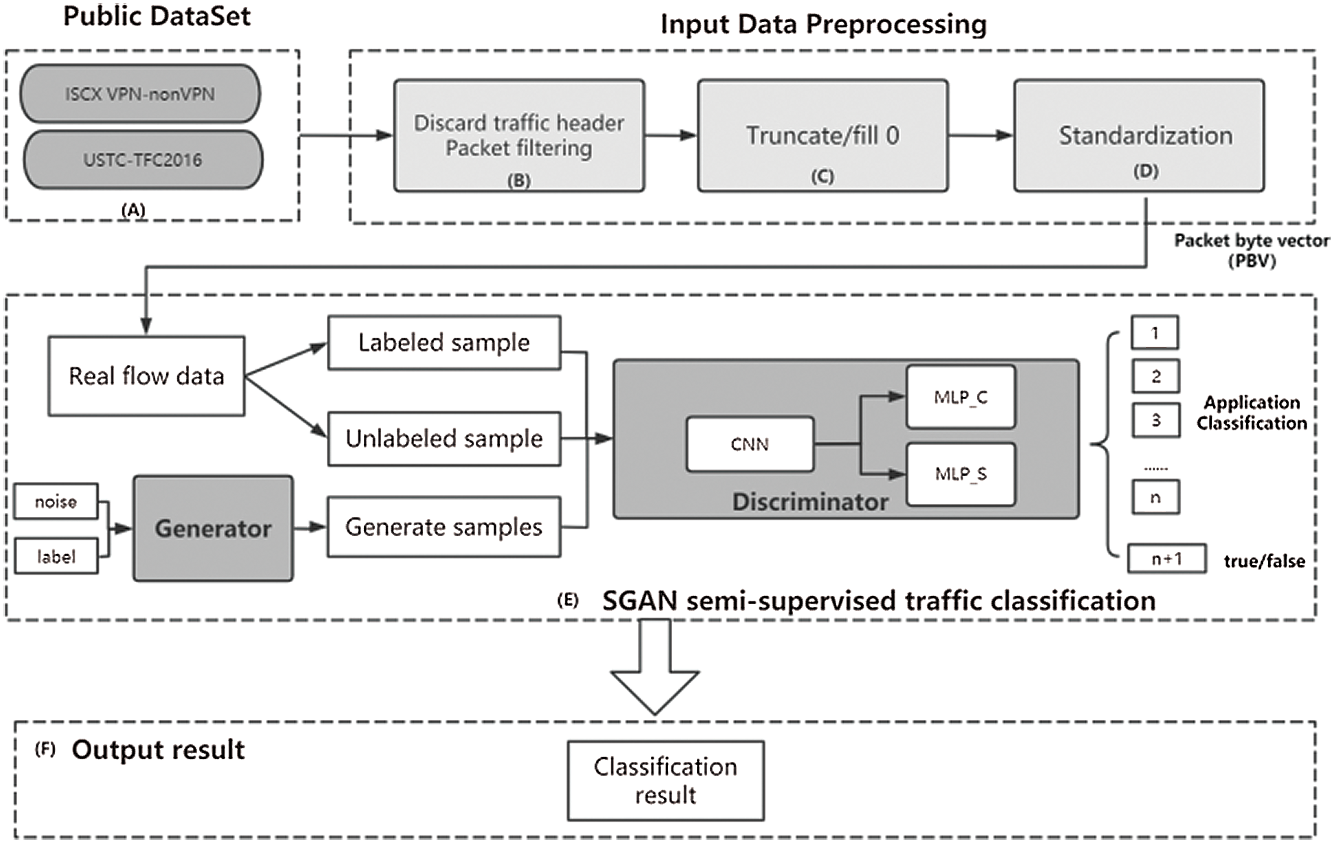
Figure 1: Overall SACGAN process
3.2 Improved Semisupervised Auxiliary Classification Generative Adversarial Network (SACGAN)
Fig. 2 shows the network structure of SACGAN. It consists of two parts: generator and discriminator. The generator receives the combined vector of noise and tags to generate traffic data. The discriminator receives real labeled data, real unlabeled data and data generated by the generator to output true and false discrimination and class labels.
During design, the network structure of the DCGAN [38], WGAN [39] and the semisupervised model [40] are referenced as follows:
a) We use a convolutional layer with strides to replace the pooling layer, use con-volution to replace the pooling layer of the discriminator network, and use de-convolution to replace the pooling layer of the generated model.
b) LeakyReLU [41] is used for activation in both the generator and discriminator, and the generator output layer uses the tanh function.
c) After updating the parameters of the discriminator, the absolute value is truncated to not exceed a fixed constant C.
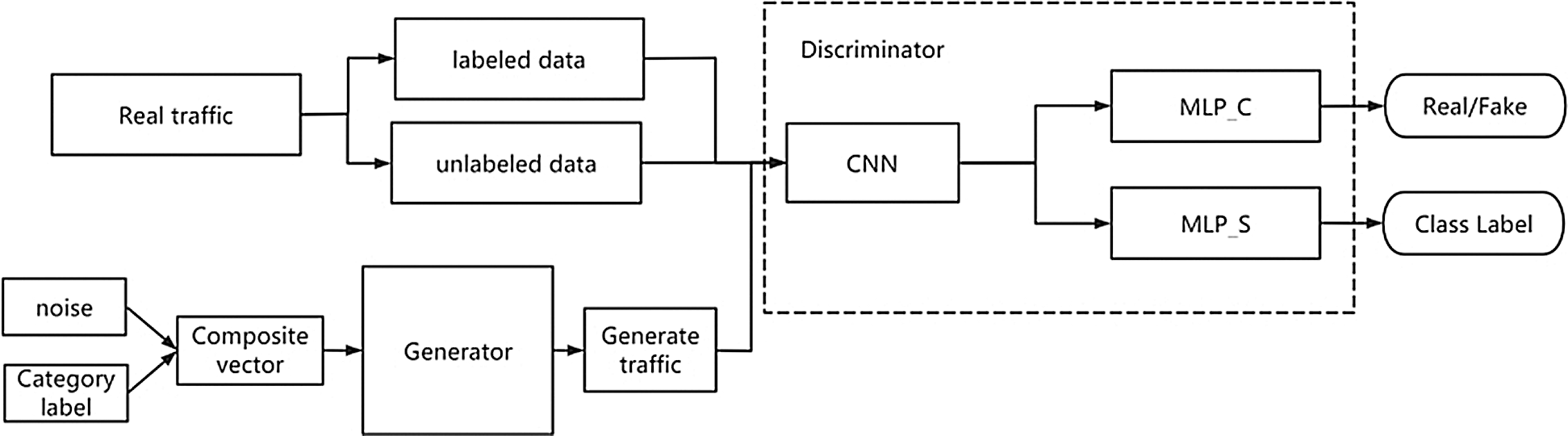
Figure 2: Network structure of the SACGAN
During implementation, the discriminator is composed of a CNN network for feature extraction and two MLP networks for classification and true-false discrimina-tion. Based on reference Salimans et al. [40], the output layer of the discriminator is built using a stacked model with shared weights. The two MLP networks multiplex the output of the CNN network. In Keras, custom functions are applied from the Lambda layer to the input layer of the network.
a. Loss function
The loss function of the SACGAN’s discriminator has two parts (classification loss and adversarial loss), as shown in formula (1). Formula 2) represents the adversarial loss, (i.e., the unlabeled loss), and formula (3) represents the classification loss, (i.e., the labeled loss):
Define
Formula (3) represents Lipschitz continuous, which means that an additional restriction is imposed on the function
In particular, we can use a set of parameters
By training the neural network, a set of
Formula (6) is the adversarial loss of the discriminator.
For the classification loss, the classification loss uses cross entropy because part of the convolutional neural network and the fully connected classifier at the end respectively complete independent classification tasks.
The discriminator is an N+1-dimensional classifier, its input is data samples, and its output is an N+1-dimensional vector:
b. Discriminator network structure
As shown in Fig. 3, the discriminator D is composed of 3 convolutional layers and 2 fully connected layers in series. The real traffic sample PBV with a length of 1480 through data preprocessing is used to form and generate a three-dimensional tensor (20*74*1) that is consistent with the flow through dimensional transformation (reshape). This tensor is then sent to the 3-layer convolution kernel
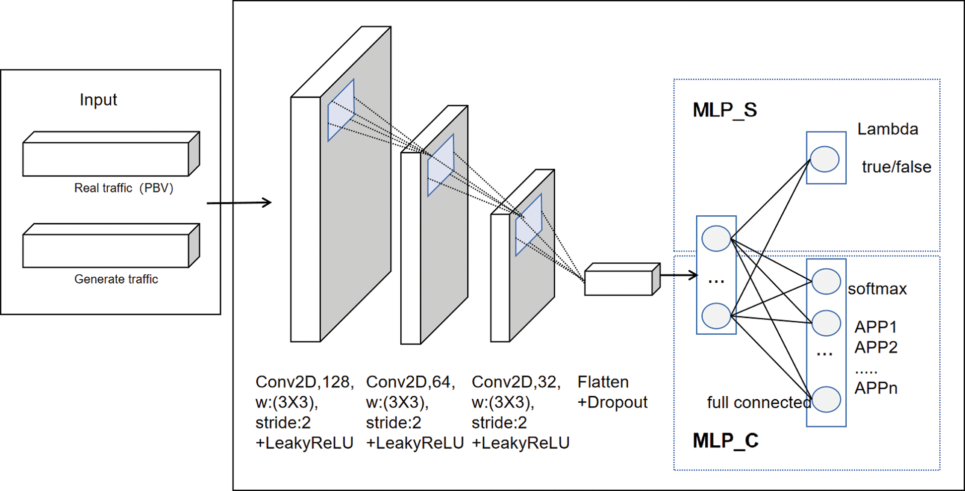
Figure 3: SACGAN discriminant network structure diagram
a. Loss function
To solve the defect of Jensen-Shannon (JS) divergence, the Wasserstein distance is used, which represents the EM distance from the real data set
b. Generator network structure
Network parameters are shown in Fig. 4. The generator G is constructed using a 1-layer deconvolution network and a 1-layer convolution network. First, 100-dimension random noise

Figure 4: SACGAN generated network structure diagram
3.3 SACGAN-Based Semisupervised Encryption Flow Identification Method
We capture original data packets in the PCAP (a file format, saved by Wireshark software) format and preprocess them as inputs for subsequent model training. Typically, PCAP preprocessing has four steps: filtering, truncation/zero padding, normalization and packet labeling.
a. Filtering:
First, we delete the ethernet header of the original data packet, data link layer information such as mac address, frame type, etc., and discard packets without application layer data. Filtering reduces the size of the input data packet. Additionally, to obtain better performance, noise is also filtered.
b. Truncation and zero padding:
To fix the input size of each data packet in the model, the TCP header is truncated to 20 bytes, and the UDP header is zero-filled to 20 bytes. The application layer data is truncated and zero-filled to form a fixed-length data packet. Because most data packets are less than or equal to 1460 bytes in length, the data length of the application layer is set to 1460 bytes. Finally, data with a length of 1480 bytes is formed.
c. Normalization
Each processed data is sent as a Packet Byte Vector (PBV). For example,
where
d. Packet labeling
Finally, the traffic that can be marked in each packet is labeled with the corresponding application to form a labeled sample, and the remainders are merged into unlabeled samples to form a data set for model training.
SACGAN training uses a combination of supervised and unsupervised losses, which can improve model learning. Because the adversarial loss
• When optimizing
• When optimizing
• During one update, the generator is updated twice, the feature extraction network is updated twice, and the branch network is updated once.
Using the gradient penalty to combat loss, the loss
The experiment in this chapter uses the ISCX VPN-nonVPN and USTC-TFC2016 data sets, as shown in Tab. 1. We select 10,000 pieces of data randomly from 9 applications of USTC-TCF2016.

For comparison, two data sets are investigated experimentally using the CNN-based classification model [14] and the SACGAN-based classification model. Before experimentation, we selected a specified number of labeled data from the data set through the code and used the remainder of the data set as unlabeled data for the experiment.
The network structure of the SACGAN’s discriminator and generator is shown in Section 3.2. On the selected data set, the batch gradient descent method is used for training, with a batch size of 256. Noise is randomly sampled from the uniform distribution of [−1, 1] with a sample size of 100. The learning rate parameter is 0.0002, and the Adam optimizer is used to optimize the loss function of the generator and the discriminator.
The CNN network structure used is shown in reference Wang et al. [14]. The batch gradient descent method is used to train the selected data set and the batch size 128. The Rmsprop optimizer is used to optimize the cross entropy loss function.
This article uses a SACGAN to perform classification experiments when there are only 1000, 2000, 3000 and 4000 labeled data in each class sample. Under the same conditions, this network is compared to the classification results of CNN to demonstrate the superior performance of the SACGAN in semisupervised encryption traffic classification.In the experiment, the data set was split into a training set and test set according to the ratio of 6:4 for cross-validation. The results in section 4.3 are based on the test set.
To evaluate the performance of the model, we use the following two types of indicators:
a. Precision and recall
False positive (FP) indicates that the traffic of noncategory C, where C refers to a specific category, is classified as category C. True Negative (TN) indicates that the traffic of noncategory C is classified as noncategory C. False negative (FN) indicates that traffic belonging to category C is classified as noncategory C. True positive (TP) indicates that traffic belonging to category C is classified as category C.
The precision rate (henceforth “precision”) is calculated using formula (11), and the recall rate (henceforth “recall”) is calculated using formula (13):
b. F1-Score
The F1score is a weighted and average of the precision and recall rates, and is used to comprehensively describe the entire index [42]. The most common formula for calculating the F1-scorescore is:
Fig. 5 shows the change in the confrontation loss on the SACGAN discriminator and generator. The confrontation loss of the discriminator gradually decreases, the confrontation loss of the generator gradually increases, and both stabilize after approximately 2000 rounds.

Figure 5: SACGAN training loss (a) Training loss of “ISCX VPN-nonVPN” dataset (b) Training loss of “USTC-TFC2016” dataset
As shown in Tab. 2, we use the SACGAN and CNN to perform classification experiments with 1000, 2000, 3000, and 4000 labeled samples, the following classification results are produced.
When the number of labeled samples is 1000, the classification accuracy of SACGAN is improved by approximately 5% compared to the CNN. When the number of labeled samples is 2000, it is improved by approximately 3% compared to the CNN. When the number of labeled samples is 3000, it is improved by below 1% compared to the CNN. When the number of labeled samples is 4000, the classification accuracy of the SACGAN is similar to that of the CNN.
Accuracy from the SACGAN remains poor regarding classification performance. We use the evaluation indicators introduced in Section 4.2 to analyze the improvement of each application more comprehensively.

a. Precision:
As shown in Fig. 6, in addition to the two applications of Facebook and Hangout, SACGAN’s precision index is basically better than that of CNN when there are labeled samples in 1000, 2000, and 3000. Among them, the improvement of AIM_Chat is greater, and the improvement is close to 20%; ICQ has improved significantly, with an increase of close to 5%; other applications such as Netflix, SCPDown, Skype, Spotify, Tort Witter, VoIP buster, and YouTube also have a small increase.

Figure 6: ISCX data set precision comparison (a) 1000 labeled data (b) 2000 labeled data (c) 3000 labeled data (d) 4000 labeled data
As shown in Fig. 7, SACGAN’s precision index is basically better than CNN when the number of labeled samples is 1000, 2000, 3000. Among them, Gmail increases by about 10% when there are 1000 labeled samples, and about 5% when there are 2000 labeled samples. BitTorrent, Outlook, and Skype improve significantly, with an increase of about 5% when there are 1000 labeled samples, and an increase of about 2% when the number of labeled samples is 2000 and 3000. Other applications also have a small improvement when there are 1000~3000 labeled samples.
b. Recall:
As shown in Fig. 8, in the experiments of 1000, 2000 and 3000 labeled samples, the recall of Gmail, netfliex, SCPDown, SFTPDown, Skype, Spotify, TorTwitter, Vimeo, VoipBuster, and YouTube are better than CNN. Among them, the improvement of Gmail is more significant, close to 20%.

Figure 7: USTC data set precision comparison (a) 1000 labeled data (b) 2000 labeled data (c) 3000 labeled data (d) 4000 labeled data

Figure 8: ISCX data set recall comparison (a) 1000 labeled data (b) 2000 labeled data (c) 3000 labeled data (d) 4000 labeled data
As shown in Fig. 9, with 1000, 2000, and 3000 labeled samples, except for BitTorrent, SACGAN’s recall index is better than CNN. Among them, the improvement of Gmail is significant, with an increase of about 5%. With 1000 and 2000 labeled samples, Outlook has improved significantly, with an increase of about 2.5%.

Figure 9: USTC data set recall comparison (a) 1000 labeled data (b) 2000 labeled data (c) 3000 labeled data (d) 4000 labeled data

Figure 10: ISCX data set recall comparison (a) 1000 labeled data (b) 2000 labeled data (c) 3000 labeled data (d) 4000 labeled data
c. F1-score:
As shown in Fig. 10, similar to the precision index, except for Facebook and Hangout, SACGAN’s f1-score index is basically better than CNN when the number of labeled samples is 1000, 2000, and 3000. Among them, AIM_Chat has a greater improvement, which is about 5% to 10%. Email, Gmail, and ICQ have been significantly improved, and the increase is large. Other applications such as Netflix, SCPDown, Skype, Spotify, TorTwitter, VoipBuster, YouTube also have a small increase.
As shown in Fig. 11 similar to the precision index, when the number of labeled samples of SACGAN is 1000, 2000, and 3000, the f1-score index is basically better than that of CNN. Among them, the improvement of Gmail is greater, which is about 3%-12%; Skype has a significant improvement, an increase of about 1%~5%; other applications also have a small increase.
From the above experimental results, it can be seen that when there is less labeled data, the classification accuracy of most applications of SACGAN is greatly improved compared to CNN.

Figure 11: USTC data set recall comparison (a) 1000 labeled data (b) 2000 labeled data (c) 3000 labeled data (d) 4000 labeled data
In this paper, we modified the network structure of the auxiliary classification generation adversarial network and modified the loss function of the generator and the discriminator. We designed a semi-supervised encrypted traffic recognition scheme based on the auxiliary classification Generative Adversarial Network. Using the proposed method and the classification method of CNN in the paper [14], classification experiments were carried out on two data sets: ISCX and USTC. The results show that under the same conditions, the proposed method has higher recognition accuracy when there are fewer labeled samples.
Acknowledgement: We thank the anonymous reviewers and editors for their very constructive comments.
Funding Statement: This work is supported by the Science and Technology Project of State Grid Jiangsu Electric Power Co., Ltd. under Grant No. J2020068.
Conflicts of Interest: The authors declare that they have no conflicts of interest to report regarding the present study.
1. K. C. Claffy, H. Braun and G. C. Polyzos, “A parameterizable methodology for Internet traffic flow profiling,” IEEE Journal on Selected Areas in Communications, vol. 13, no. 8, pp. 1481–1494, 1995. [Google Scholar]
2. R. Gu, H. Wang, Y. Sun and Y. Ji, “Fast traffic classification using joint distribution of packet size and estimated protocol processing time,” IEICE Transactions on Information and System, vol. 93, no. 11, pp. 2944–2952, 2010. [Google Scholar]
3. S. H. Yeganeh, M. Eftekhar, Y. Ganjali, R. Keralapura and A. Nucci, “CUTE: Traffic classification using terms,” in Proc. ICCCN, Munich, MUC, Germany, pp. 1–9, 2012. [Google Scholar]
4. H. A. H. Ibrahim, S. M. Nor and H. A. Jamil, “Online hybrid internet traffic classification algorithm based on signature statistical and port methods to identify internet applications,” in Proc. ICCSCE, Penang, PEN, Malaysia, pp. 185–190, 2013. [Google Scholar]
5. M. Conti, L. V. Mancini, R. Spolaor and N. V. Verde, “Can’t you hear me knocking: Identification of user actions on android apps via traffic analysis,” in Proc. CODASPY, New York, NY, USA, pp. 297–304, 2019. [Google Scholar]
6. D. Kim, G. Shin and M. Han, “Analysis of feature importance and interpretation for malware classification,” Computers, Materials & Continua, vol. 65, no. 3, pp. 1891–1904, 2020. [Google Scholar]
7. C. Du, S. Liu, L. Si, Y. Guo and T. Jin, “Using object detection network for malware detection and identification in network traffic packets,” Computers, Materials & Continua, vol. 64, no. 3, pp. 1785–1796, 2020. [Google Scholar]
8. C. Mo, W. Xiaojuan, H. Mingshu, J. Lei and K. Javeed, “A network traffic classification model based on metric learning,” Computers, Materials & Continua, vol. 64, no. 2, pp. 941–959, 2020. [Google Scholar]
9. W. Wang, Y. Sheng, J. Wang, X. Zeng, X. Ye et al., “HAST-IDS: Learning hierarchical spatial-temporal features using deep neural networks to improve intrusion detection,” IEEE Access, vol. 6, pp. 1792–1806, 2018. [Google Scholar]
10. G. Aceto, D. Ciuonzo, A. Montieri and A. Pescapé, “Mobile encrypted traffic classification using deep learning,” in Proc. TMA, Vienna, VIE, AT, pp. 1–8, 2018. [Google Scholar]
11. G. Aceto, D. Ciuonzo, A. Montieri and A. Pescapé, “Mobile encrypted traffic classification using deep learning: Experimental evaluation, lessons learned and challenges,” IEEE Transactions on Network and Service Management, vol. 16, no. 2, pp. 445–458, 2019. [Google Scholar]
12. M. Lopez-Martin, B. Carro, A. Sanchez-Esguevillas and J. Lloret, “Network traffic classifier with convolutional and recurrent neural networks for internet of things,” IEEE Access, vol. 5, pp. 18042–18050, 2017. [Google Scholar]
13. J. Höchst, L. Baumgärtner, M. Hollick and B. Freisleben, “Unsupervised traffic flow classification using a neural autoencoder,” in Proc. LCN, Singapore, SGP, pp. 523–526, 2017. [Google Scholar]
14. P. Wang, F. Ye, X. Chen and Y. Qian, “Datanet: Deep learning based encrypted network traffic classification in SDN home gateway,” IEEE Access, vol. 6, pp. 55380–55391, 2018. [Google Scholar]
15. I. J. Goodfellow, “Generative adversarial networks,” arXiv e-prints, arXiv:1406.2661, 2014. [Google Scholar]
16. C. Ledig, L. Theis, F. Huszar, J. Caballero, A. Cunningham et al., “Photo-realistic single image super-resolution using a generative adversarial network,” in Proc. CVPR, Honolulu, HNL, USA, pp. 105–114, 2017. [Google Scholar]
17. H. W. Dong, W. Y. Hsiao, L. C. Yang and Y. H. Yang, “MuseGAN: Multi-track sequential generative adversarial networks for symbolic music generation and accompaniment,” in Proc. AAAI, New Orleans, NO, USA, pp. 117–125, 2018. [Google Scholar]
18. O. Olabiyi, A. Salimov, A. Khazane and E. T. Mueller, “Multi-turn dialogue response generation in an adversarial learning framework,” arXiv e-prints, arXiv:1805.11752, 2018. [Google Scholar]
19. F. Zhang, H. Zhao, W. Ying, Q. Liu, A. Noel et al., “Human face sketch to rgb image with edge optimization and generative adversarial networks,” Intelligent Automation & Soft Computing, vol. 26, no. 4, pp. 1391–1401, 2020. [Google Scholar]
20. X. Chen, J. Chen and Z. Sha, “Edge detection based on generative adversarial networks,” Journal of New Media, vol. 2, no. 2, pp. 61–77, 2020. [Google Scholar]
21. W. Hu and Y. Tan, “Generating adversarial malware examples for black-box attacks based on GAN,” arXiv e-prints, arXiv:1702.05983, 2017. [Google Scholar]
22. J. Y. Kim, S. J. Bu and S. B. Cho, “Malware detection using deep transferred generative adversarial networks,” in Proc. ICONIP, Guangzhou, GZ, China, pp. 556–564, 2017. [Google Scholar]
23. Z. Lin, Y. Shi and Z. Xue, “IDSGAN: Generative adversarial networks for attack generation against intrusion detection,” arXiv e-print, arXiv:1809.02077, 2018. [Google Scholar]
24. L. Vu, C. Thanh Bui and U. Nguyen, “A deep learning based method for handling imbalanced problem in network traffic classification,” in Proc. SoICT, Nha Trang City, NTC: Viet Nam, pp. 333–339, 2017. [Google Scholar]
25. G. Douzas and F. Bacao, “Effective data generation for imbalanced learning using conditional generative adversarial networks,” Expert Systems with Applications, vol. 91, no. 2, pp. 464–471, 2018. [Google Scholar]
26. M. Arjovsky and L. Bottou, “Towards principled methods for training generative adversarial networks,” arXiv e-prints, arXiv:1701.04862, 2017. [Google Scholar]
27. M. Arjovsky, S. Chintala and L. Bottou, “Wasserstein generative adversarial networks,” in Proc. ICML, Sydney, SYD, AUS, pp. 214–223, 2017. [Google Scholar]
28. U. Fiore, A. De Santis, F. Perla, P. Zanetti and F. Palmieri, “Using generative adversarial networks for improving classification effectiveness in credit card fraud detection,” Information Sciences, vol. 479, no. 4, pp. 448–455, 2019. [Google Scholar]
29. M. Zheng, T. Li, R. Zhu, Y. H. Tang, M. J. Tang et al., “Conditional wasserstein generative adversarial network-gradient penalty-based approach to alleviating imbalanced data classification,” Information Sciences, vol. 512, pp. 1009–1023, 2020. [Google Scholar]
30. A. Rasmus, M. Berglund, M. Honkala, H. Valpola and T. Raiko, “Semi-supervised learning with ladder networks,” in Advances in neural information processing systems, pp. 3546–3554, 2015. [Google Scholar]
31. R. Johnson and T. Zhang, “Supervised and semi-supervised text categorization using LSTM for region embeddings,” in Proc. ICML, New York, NY, USA, pp. 526–534, 2016. [Google Scholar]
32. S. Rezaei and X. Liu, “How to achieve high classification accuracy with Just a few labels: A semi-supervised approach using sampled packets,” arXiv e-prints, arXiv:1812.09761, 2018. [Google Scholar]
33. T. Salimans, I. Goodfellow, W. Zaremba, V. Cheung, A. Radford et al., “Improved techniques for training GANs,” arXiv e-prints, arXiv:1606.03498, 2016. [Google Scholar]
34. Z. Dai, Z. Yang, F. Yang and W. W. Cohen, “Good semi-supervised learning that requires a bad GAN,” in Proc. NIPS, New York, NY, USA, pp. 6513–6523, 2017. [Google Scholar]
35. J. T. Springenberg, “Unsupervised and semi-supervised learning with categorical generative adversarial networks,” arXiv e-prints, arXiv:1511.06390, 2015. [Google Scholar]
36. A. S. Iliyasu and H. Deng, “Semi-supervised encrypted traffic classification with deep convolutional generative adversarial networks,” IEEE Access, vol. 8, pp. 118–126, 2020. [Google Scholar]
37. A. Odena, C. Olah and J. Shlens, “Conditional image synthesis with auxiliary classifier GANs,” arXiv e-prints, arXiv:1610.09585, 2016. [Google Scholar]
38. A. Radford, L. Metz and S. Chintala, “Unsupervised representation learning with deep convolutional generative adversarial networks,” arXiv e-prints, arXiv:1511.06434, 2015. [Google Scholar]
39. M. Arjovsky, S. Chintala and L. Bottou, “Wasserstein GAN,” arXiv e-prints, arXiv:1701.07875, 2017. [Google Scholar]
40. T. Salimans, I. Goodfellow, W. Zaremba, V. Cheung and A. Radford, “Improved techniques for training GANs,” arXiv e-prints, arXiv:1606.03498, 2016. [Google Scholar]
41. B. Xu, N. Wang, T. Chen and M. Li, “Empirical evaluation of rectified activations in convolutional network,” arXiv e-print, arXiv:1505.00853, 2015. [Google Scholar]
42. H. Kim, K. C. Claffy, M. Fomenkov, D. Barman, M. Faloutsos et al., “Internet traffic classification demystified: Myths, caveats and the best practices,” in Proc. CoNEXT, Madrid, Spain,2008. [Google Scholar]
 | This work is licensed under a Creative Commons Attribution 4.0 International License, which permits unrestricted use, distribution, and reproduction in any medium, provided the original work is properly cited. |