DOI:10.32604/csse.2022.018430
| Computer Systems Science & Engineering DOI:10.32604/csse.2022.018430 | |
| Article |
A Particle Swarm Optimization Based Deep Learning Model for Vehicle Classification
1Department of Computer Science, College of Computer Engineering and Sciences in Al-Kharj, Prince Sattam bin Abdulaziz University, P.O. Box 151, Al-Kharj, 11942, Saudi Arabia
2Department of Computer Science, COMSATS University Islamabad, Wah Cantt, 47010, Pakistan
3University of Jeddah, College of Computer Science and Engineering Department of Cybersecurity, Jeddah, 21959, Saudi Arabia
*Corresponding Author: Adi Alhudhaif. Email: a.alhudhaif@psau.edu.sa
Received: 09 March 2021; Accepted: 30 April 2021
Abstract: Image classification is a core field in the research area of image processing and computer vision in which vehicle classification is a critical domain. The purpose of vehicle categorization is to formulate a compact system to assist in real-world problems and applications such as security, traffic analysis, and self-driving and autonomous vehicles. The recent revolution in the field of machine learning and artificial intelligence has provided an immense amount of support for image processing related problems and has overtaken the conventional, and handcrafted means of solving image analysis problems. In this paper, a combination of pre-trained CNN GoogleNet and a nature-inspired problem optimization scheme, particle swarm optimization (PSO), was employed for autonomous vehicle classification. The model was trained on a vehicle image dataset obtained from Kaggle that has been suitably augmented. The trained model was classified using several classifiers; however, the Cubic SVM (CSVM) classifier was found to outperform the others in both time consumption and accuracy (94.8%). The results obtained from empirical evaluations and statistical tests reveal that the model itself has shown to outperform the other related models not only in terms of accuracy (94.8%) but also in terms of training time (82.7 s) and speed prediction (380 obs/sec).
Keywords: Vehicle classification; intelligent transport system; deep learning; constrained machine learning; particle swarm optimization; CNN GoogleNet
Research in various real-world domains has provided next-generation advancements and solutions to problems. These advancements have also had an impact on the automobile industry. In the past, it was easy to differentiate between the relatively few vehicles makes and models simply by looking at them once. The current variety of vehicles, however, is huge in terms of models and makes, which makes classifying them a challenging task. This challenge is a critical image analysis problem and requires an intelligent traffic classification system to differentiate between types of vehicles such as cars, trucks, ambulances, and bicycles. Vehicle classification is an important domain in the field of image classification and can be used in different applications for solving critical real-world problems such as traffic analysis, traffic surveillance, and traffic security management [1]. The challenge in vehicle classification is the diversity of vehicle colors, models, and makes. The massive variation in vehicles these days makes it tough for a human to classify different vehicles just by looking at them because most vehicles are similar in build and shape but vary slightly in some respects. For an algorithm that is to be run on computer, this challenge becomes even bigger [2]. With the progress in research, various methodologies have been proposed that make this classification task fairly easier to some extent. These methodologies are classified into two categories: handcrafted and deep learning methods. Each has benefits and limitations depending upon the nature of data and problem statement [3].
Earlier, when the field of artificial intelligence did not receive much attenion, various conventional and handcrafted methods were used for image classification that demanded a lot of manual human contribution, consumed much time, wasted a great many resources, and yielded poor results. Recent expansions in the field of machine learning, artificial intelligence, and deep learning have guided this research to a new dimension [4]. Convolutional neural networks are products of deep learning that are widely used in most image processing problems.
The concept of CNN was provided by Fukushima et al. and modified by LeChun et al. A CNN is a collection of multiple layers comprising of neurons regularized together in a compact way. A deep convolutional neural network consists of multiple convolutional layers, pooling layers, activation layers, rectified linear units (ReLU), flatten layers and fully connected layers. CNNs can be trained on large datasets where they extract features automatically using their embedded layers [5]. Fig. 1 illustrates the basic structure of a simple CNN.
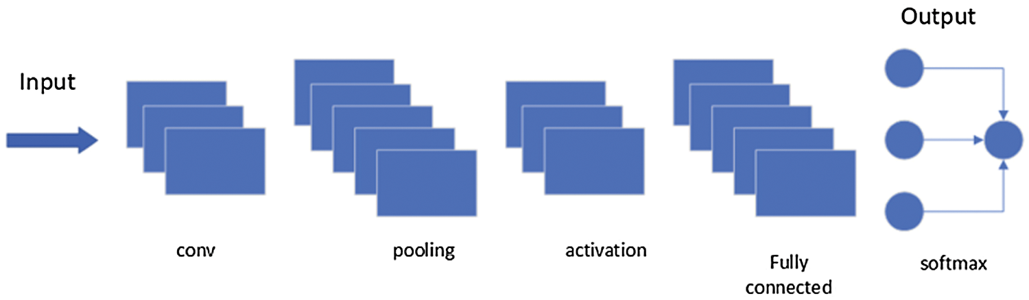
Figure 1: A standard Convolutional Neural Network (CNN) architecture [6]
The convolutional layers of a CNN are used to extract all important features, including shape, edges, lines, points, color, and textures. The input taken by the convolutional layer is a normal three-dimensional (a x b x c) RGB image where a indicates height, b indicates the width, and c indicates the image’s total number of channels. The convolutional layer outputs a feature map comprising all the extracted and learned features from the image dataset [7].
Taking the feature map generated by the convolutional layer as an input, the pooling layer reduces the computational burden on the network by optimizing parameters obtained from the features maps and thus helps control overfitting [8]. The activation function determines whether to activate a particular neuron depending upon the relevancy of the information that it is receiving, which brings a non-linearity to the network. Various activation functions are used for solving different contextual problems, such as sigmoid function, rectified linear unit (ReLU) function, and tangent hyperbolic (tanh) function [9].
A fully connected layer combines all the values coming from the input into a final variant of the results to proceed to classification stage. At the end, the classification is performed with the help of the SoftMax layer, and the probabilities are calculated for each individual class [10].
This paper proposes a particle swarm optimization-(PSO) based deep-learning approach for vehicle image classification. The dataset used for this purpose is obtained from Kaggle and contains eight different classes of vehicles, which are maintained and balanced using augmentation. The pre-trained deep-learning model GoogleNet is used for feature learning and extraction from the input images. The features are then optimized and reduced using the nature-based optimization algorithm PSO. The derived features from the model are passed on to the classification learner, where different classifiers are implemented. The CSVM classifier outperforms all others with an accuracy of 94.8% while maintaining brisk speed on the given dataset.
The rest of the paper is organized as follows. Section 2 presents the review of relevant techniques that have addressed vehicle classification problems. Section 3 provides detailed insight into our proposed model. Section 4 describes our experiments and reports the results. Finally, Section 5 provides our conclusions and discusses possible future directions.
Lu et al. [11] presented an image dataset, Frontal-103, for fine-grained vehicle classification that contains frontal vehicle images. The dataset comprises 65,433 images taken from the Internet containing 1759 vehicle models that are further categorized in 103 vehicle makes. The images are labelled as one of eight viewpoints: left, right, front, rear, left front, right front, left rear, or right rear. The proposed dataset is trained and tested on various convolutional neural networks (CNNs), namely AlexNet, VGG-16, VGG-19, ResNet18, ResNet50, and DenseNet121 where ResNet50 obtained the maximum overall accuracy (91.28%). Castro et al. [12] created a dataset using free images on the internet. The dataset contains 14,144 images in total with 10,880 images for training and 3264 images for validation, categorized in five classes: Sedan, Buses, SUV, Pickup trucks, and Motorcycles. A novel CNN proposed for classification consists of five convolutional layers, five max pooling layers, and two fully connected layers, which takes fewer parameters than standard CNNs and is resource friendly. The proposed model shows an accuracy of 96% on the dataset used.
Garcia et al. [13] made use of a dataset from Stanford university dataset holding 16,000 vehicle images with the aim to recognize the current view perspective of vehicles, including front view, rear view, side view and tilted view. The data is divided into exactly these four perspective classes with 735 images in frontal view, 274 images in rear view, 1020 images in side view, and 13,907 images in tilted view. A deep learning model was constructed using Keras and TensorFlow libraries with Python and comprises various layers including convolutional layers, ReLU, and a SoftMax layer for classification. The accuracy obtained with the proposed model was 88%. Soon et al. [14] used the BIT-Vehicle dataset, which consists of 9850 vehicle images in six vehicle categories: bus, minivan, microbus, sedan, SUV and truck. Images containing multiple images were segmented, and the final numbers of images for each vehicle class were 558 bus, 883 microbus, 476 minivan, 5922 sedan, 1392 SUV, and 822 truck images. A novel PCA convolutional network (PCN) was used in which the time-consuming back propagation approach of CNN was resolved by formulating the convolutional filters with the help of principal component analysis (PCA), which reduces the training burden and produces flexible features considering various aspects. This approach yields an average accuracy of above 88.35% in various conditions. Sowmya et al. [15] used a custom made dataset containing 5500 images of buses, trucks, and motorcycles obtained from various internet resources and standard ImageNet datasets. 3000 images are kept for training, 1500 for validation, and 1000 for testing purposes.
Dehkordi et al. [16] obtained a dataset comprising images and videos by means of a roadside camera. The dataset consists of 7000 images in frontal and rear-view perspective. The work calculates the coordinates of the vanishing point using vehicle motion estimation. It then analyses the structure, shadows, and color of the vehicle and compares it to the trained benchmark vehicle images to find out the exact vehicle model and make. Bag of words feature extraction was used for this process. The model achieves an average accuracy of 89.5%. Dabiri et al. [17] proposed deep learning based classification model CNN-VC for vehicle discrimination based on vehicle GPS trajectory. In this model, the vehicle’s motion mirage while moving is obtained using a navigation module which delivers the accurate GPS coordinates and distance. The model then provides the accurate vehicle class prediction based on location and distance data gathered from GPS and navigation sensors, obtaining an average accuracy of 85.6%.
On the other hand, in this paper we propose a PSO-based deep learning approach for vehicle image classification. The dataset used for this purpose is obtained from Kaggle and contains eight different vehicle classes that are maintained and balanced using augmentation. The pre-trained deep learning model GoogleNet is used for feature learning and extraction from the input images. The features are then optimized and reduced using nature-based optimization algorithm PSO. The derived features from the model are passed on to the classification learner which implements various classifiers. The CSVM classifier outperforms all others with an accuracy of 94.8% while maintaining brisk speed on the given dataset.
In the proposed work, a nature-inspired feature optimizer, PSO, is combined with the pre-trained deep model GoogleNet to create a classification model for vehicle image classification. The eight-vehicle-type Kaggle dataset, in its raw form, is unbalanced and unmaintained; we balance, arrange, and maintain it by rotating it 90, 180, and 135 degrees and flipping it horizontally and vertically. The images are then resized at 224 x 224 dimensions to indent scale uniformity within the whole dataset. The guided filter is used in the preprocessing stage for data enhancement. The preprocessed images are passed on to the pre-trained GoogleNet model for feature learning and extraction. The learned features are then optimized with the help of particle swarm optimization (PSO). The optimized features are given to various classifiers and are tested for a number of performance parameters. The quadratic SVM classifier outperforms all others in terms of accuracy (94.8%) and time consumption. The proposed model schema is illustrated in Fig. 2.
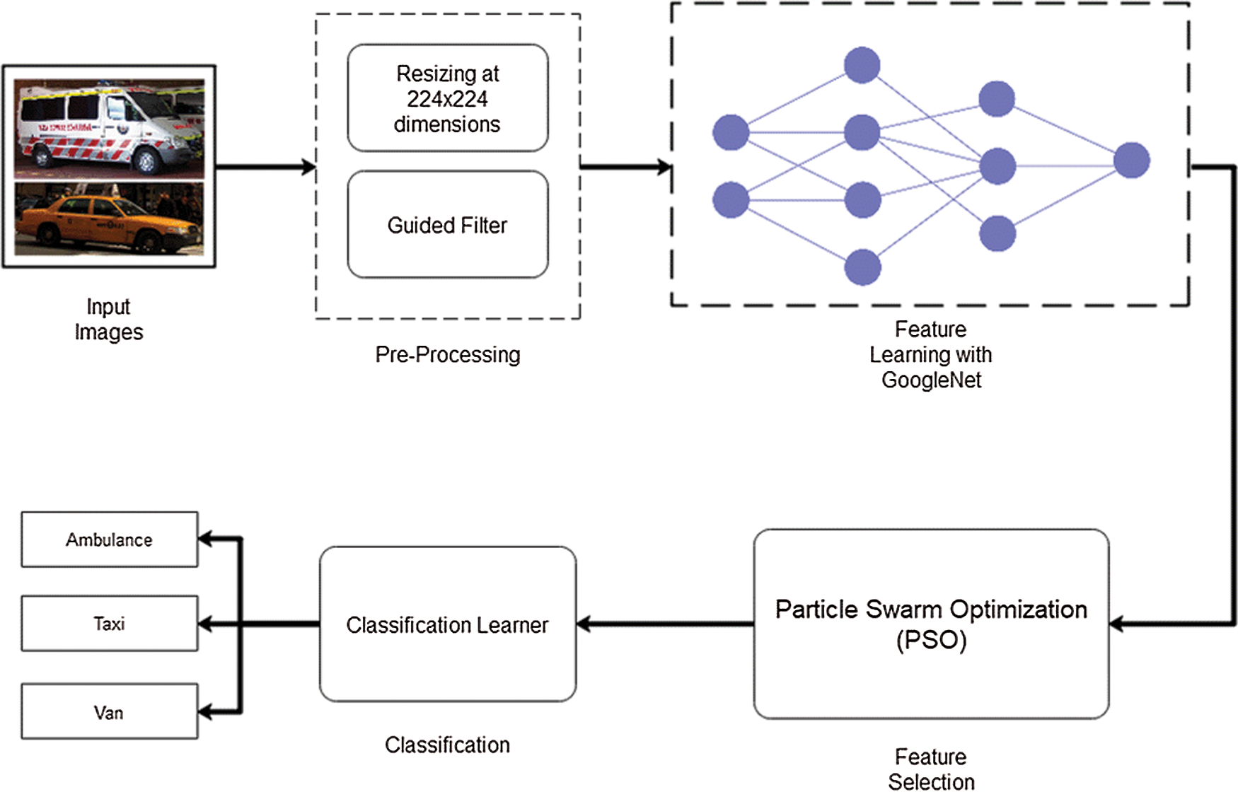
Figure 2: Architecture of proposed model
3.1 Data Acquisition and Pre-Processing
The Kaggle dataset used in the proposed work, which originally contained seventeen different vehicle classes, has been reduced to eight: ambulance, bicycle, boat, bus, helicopter, tank, taxi and van. Apart from these vehicles, other uncommon and unnecessary vehicles classes have been removed to reduce complexity and computational burden. The images are in RGB color channel and are non-uniform with different scales. The dataset contains images obtained in various random perspectives with side, rear, and frontal views. Data classes can be visualized in Fig. 3.
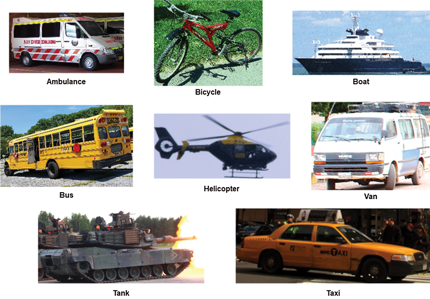
Figure 3: Dataset images
The dataset in its raw form is unbalanced and biased and is rearranged and balanced using image augmentation techniques, namely image rotation at 90, 180, and 135 degrees and vertical and horizontal image flipping, as shown in Fig. 4. The final dataset contains 4000 total images divided into eight different vehicle classes, each of which contains 500 images.
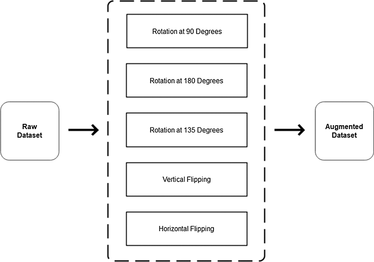
Figure 4: Data augmentation
The dataset contains images that are in RGB color channels and/or vary in terms of scale and size. To create uniformity and harmony among all the dataset images, all the images are resized to 224 × 224 dimensions. Resizing creates a biasness among data and reduces the computational burden for the deep convolutional neural network to which the images will be passed as an input in the next stage. Fig. 5 highlights the pre-processing steps carried out in ongoing work.
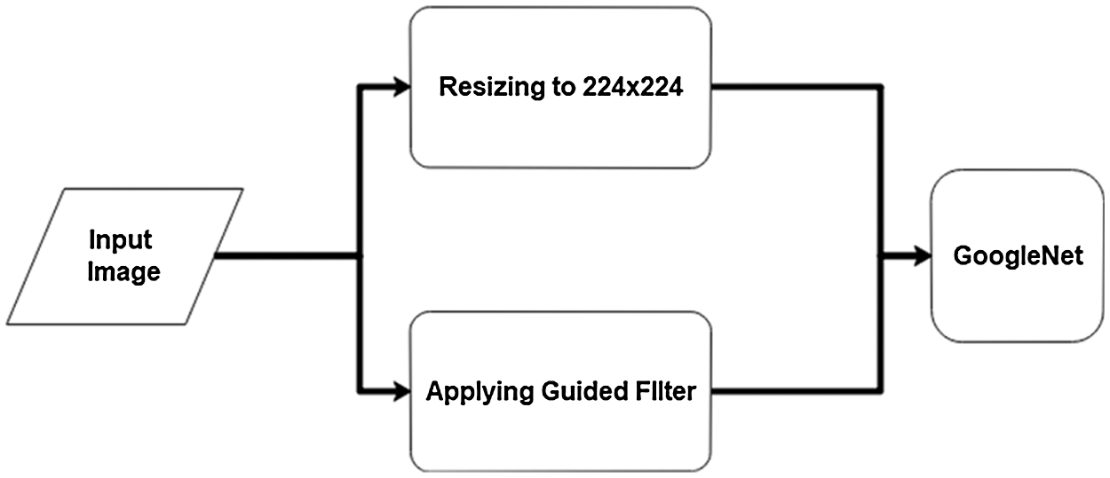
Figure 5: Preprocessing
After data acquisition, arrangement, balancing, maintenance, and processing, the next stage is feature extraction. In the proposed work, feature learning and extraction is performed by the pre-trained deep convolutional neural network GoogleNet. The following sections explain this process. GoogleNet is a 22-layer deep CNN trained on the ImageNet dataset, a vast benchmark dataset containing a wide variety of images belonging to different objects. This pre-trained model can classify images into 1000 object categories. It takes input images in size of 224 x 224 dimensions [18]. Fig. 5 shows an approximate illustration of GoogleNet. It contains a large number of small convolutional layers that reduce computational burden and perform deep feature learning. The standard GoogleNet architecture is highlighted in Fig. 6.
In the proposed work, a total of 4000 images (see Tab. 1), categorized in eight different classes with 500 images in each class, are given to the pre-trained GoogleNet model, which uses its deep layers to perform feature learning and extraction. In the proposed model, classification is not performed by the SoftMax layer of GoogleNet; rather, extracted features are taken out of the model right before they move to the last classification layer. This is done so that features are optimized using particle swarm optimization (PSO) and then classified manually using the classification learner.
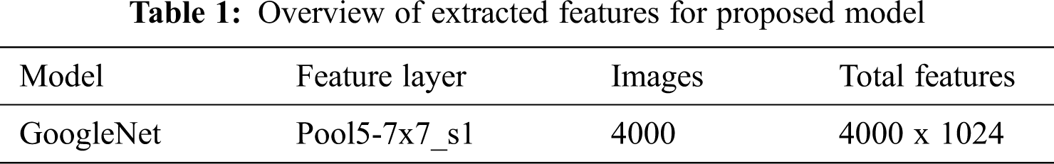
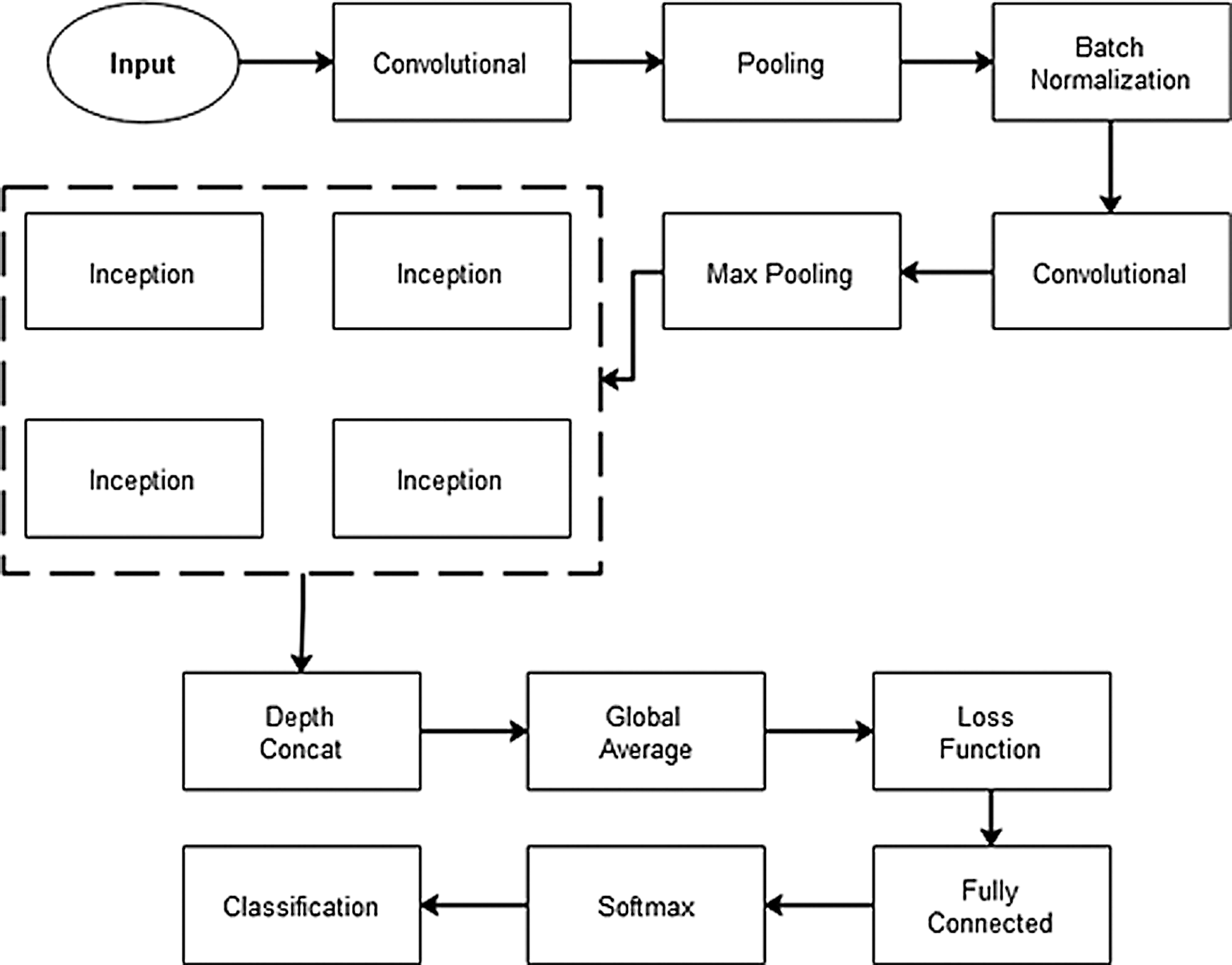
Figure 6: GoogleNet architecture [19]
The extracted features from the GoogleNet are numerous, which can create computational burden for the classifier and produce complexity in terms of time and space. This many features can also lead to inaccuracy and false prediction. Therefore, to reduce and optimize these obtained features, a feature selector is implemented in the proposed work: Particle Swarm Optimization (PSO).
PSO is a population-based algorithm that works on the idea and inspiration of bird flocks, fish schools, and other swarms. The name “Particle Swarm Optimization” comprises three words: Particle, which denotes a single entity or solution of a huge problem; Swarm, which denotes any problem that is computationally very expensive and cannot be solved without optimization; and Optimization, which marks the finding of a best solution for a given problem [20]. PSO is a stochastic approach-based algorithm that finds the solution of a given problem randomly without following any specific steps. To begin the solution formulation process in PSO, a swarm of agents is allocated that starts finding the optimal solution of the given problem in swarms on the basis of fitness value estimation in each iteration. When any agent finds out the solution, it updates its neighbors, which update their fitness values and distance vectors accordingly [21].
Particles change and update their position, velocity and fitness values using Eq. (1). Where “vel” indicates velocity of the particle, “const” indicates acceleration constant, rand function is used for random movement of swarm, and part indicates particle identity [22].
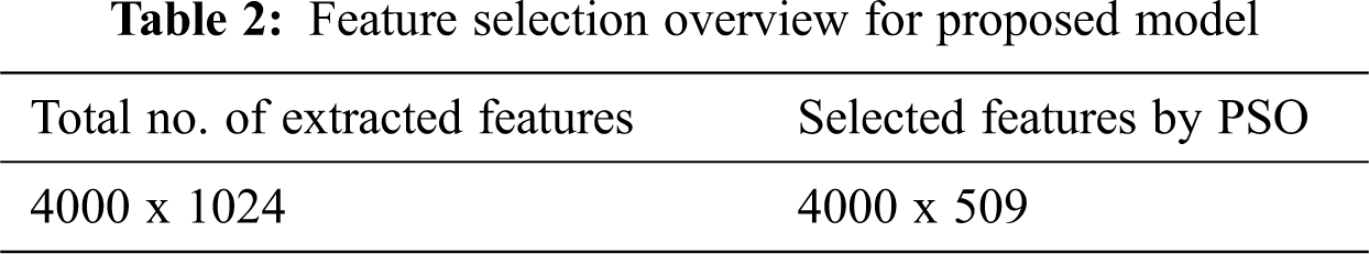
Tab. 2 shows an overview of selected features and their correspondence to the extracted features. GoogleNet extracts a total of 1024 features from 4000 images provided to it. When these features are passed on to the PSO, it optimizes them to 509 features, selecting those most suitable and rectifying others.
In the last stage, classification, the finalized selected features are classified and tested. In the proposed model, the features learned by the GoogleNet are taken out of the last pooling layer to prevent the SoftMax layer from classifying them. These features are optimized using PSO. The selected features are then passed onto the classification learner where they are tested and classified using various classifiers, including tree classifiers fine tree (FT) and medium tree (MT), linear discriminant classifier (LD), k-nearest neighbor classifier Cosine KNN (CSKNN), and support vector machine (SVM) classifiers. The support vector machine classifiers stand out in terms of accuracy and time consumption; the Cubic SVM (CSVM) classifier provides an accuracy of 94.8% while maintaining an equally good time consumption rate, which is better than other classifiers and works on the dataset used.
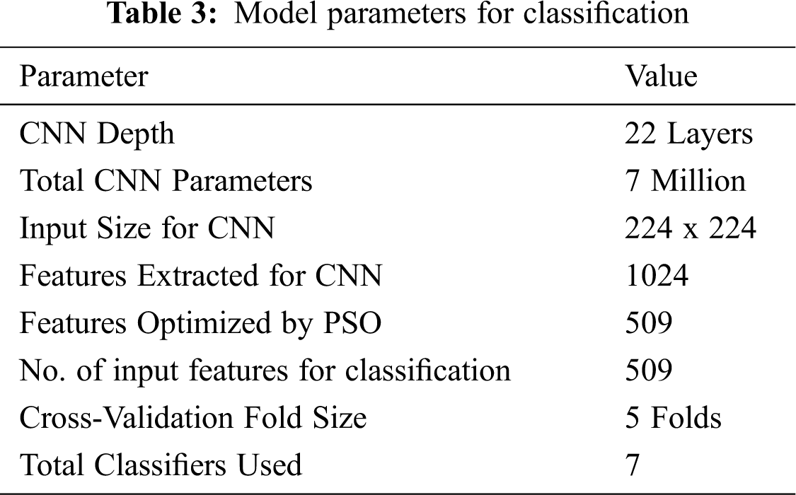
In the proposed work, appropriate data augmentation and preprocessing steps are performed on the raw vehicle dataset. The finalized data set contains a total of 4000 images categorized into eight different vehicle classes. The preprocessed images are given to the pre-trained GoogleNet convolutional neural network for feature learning. Extracted features are then optimized using the nature-based optimization model, the PSO algorithm, and passed onto the classification learner to be classified using various classifiers. A few main training parameters are highlighted in Tab. 3.
The experiments are performed on Intel Core i5 with 8GB RAM running on Windows 10 OS. The system houses a 256 GB solid-state drive (SSD) on which the MATLAB 2020a version has been installed.
Tab. 4 displays the results of various classifiers that classify data based on the optimized features given to them. The results are compared and evaluated with the help of evaluation measures recall and kappa. The Cubic SVM classifier yields an accuracy of 94.8%, far better than that of other classifiers used. Fig. 7 shows the confusion matrix for the proposed model where the highest accuracy yielding model CSVM is in operation. Fig. 8 demonstrates the scatter plotting for CSVM. The data division is visualized in the plot, which highlights various results affecting data artifacts and parameters; the proposed model provides the quality results.
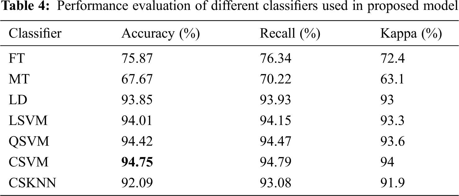
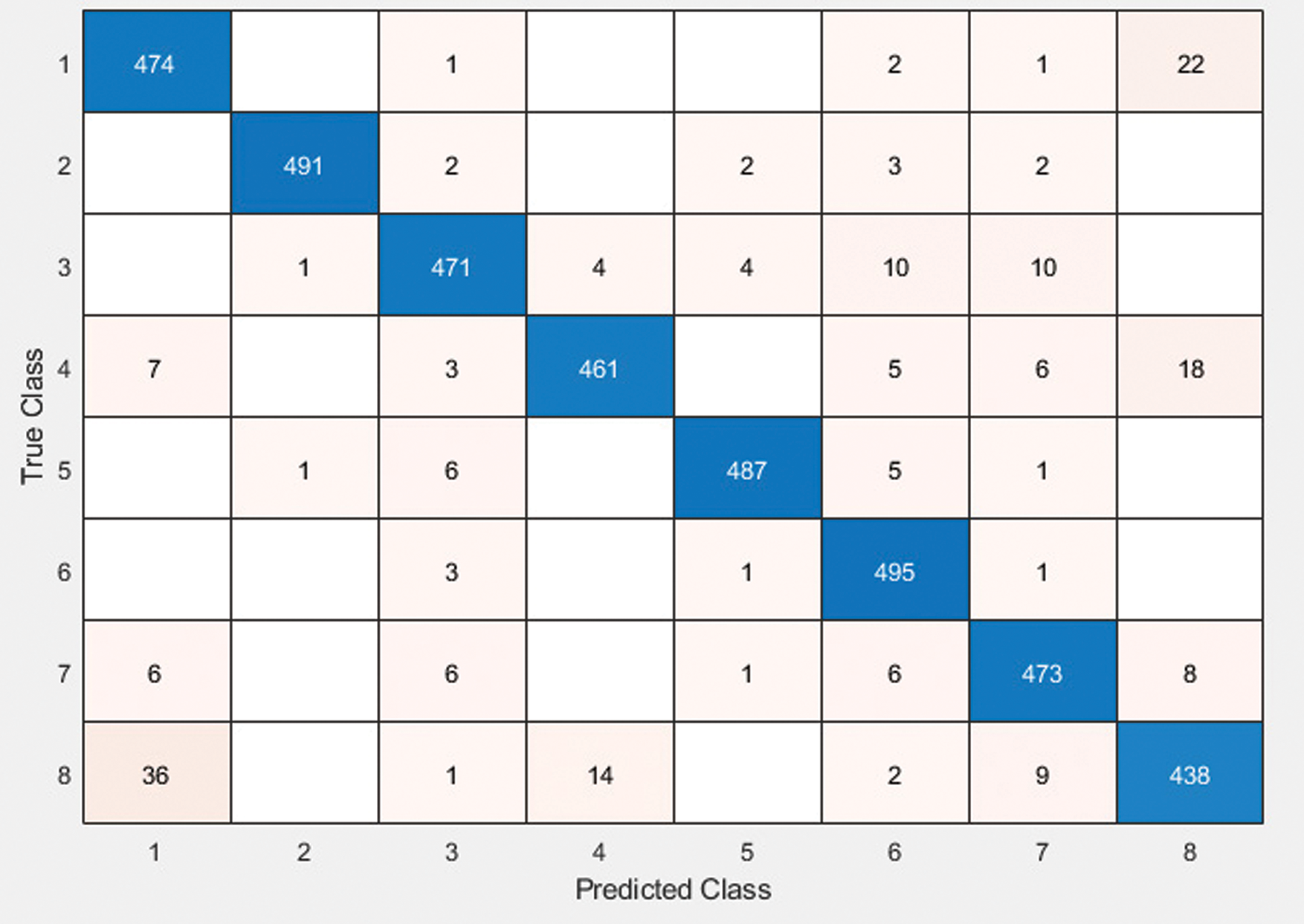
Figure 7: Confusion matrix for CSVM
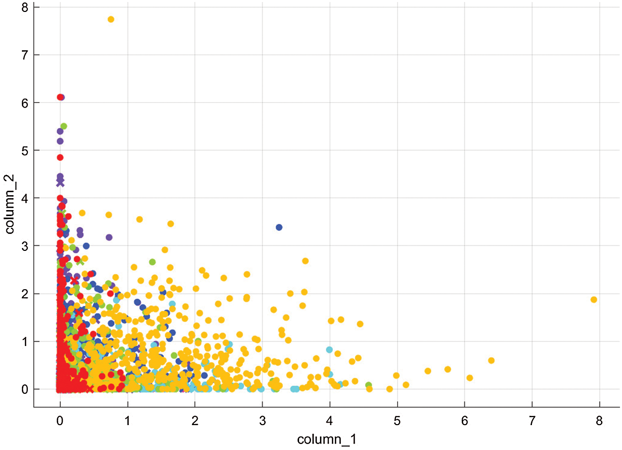
Figure 8: Scatter plot for CSVM
Fig. 9 shows the training time comparison of various classifiers. The prediction rate for most of the classifiers is extremely fast, but they show reduced accuracy. The CSVM classifier provides the best balance of accuracy and time exertion and was therefore chosen for the proposed model.
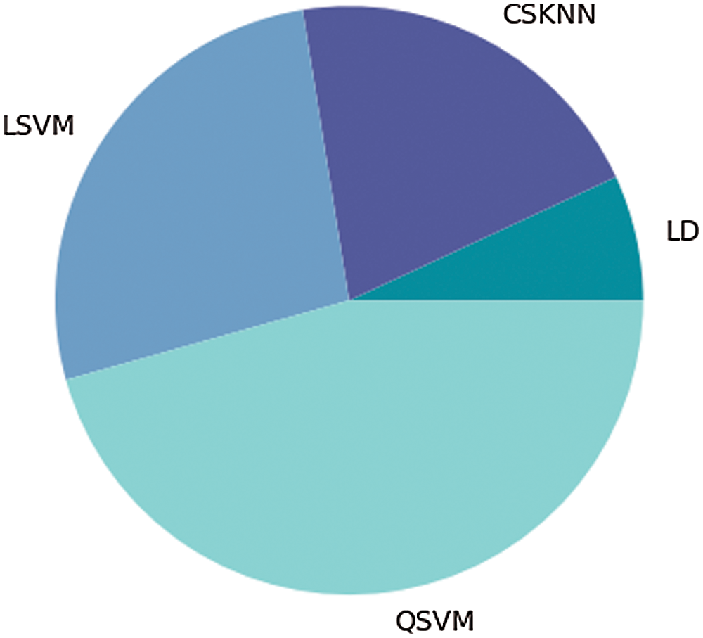
Figure 9: Training time comparison among various classifiers
Fig. 10 shows the prediction speed comparison between different classifiers. The linear discriminant classifier provides the best prediction speed with 3100 observations/sec, thus providing fast prediction although compromising on accuracy.
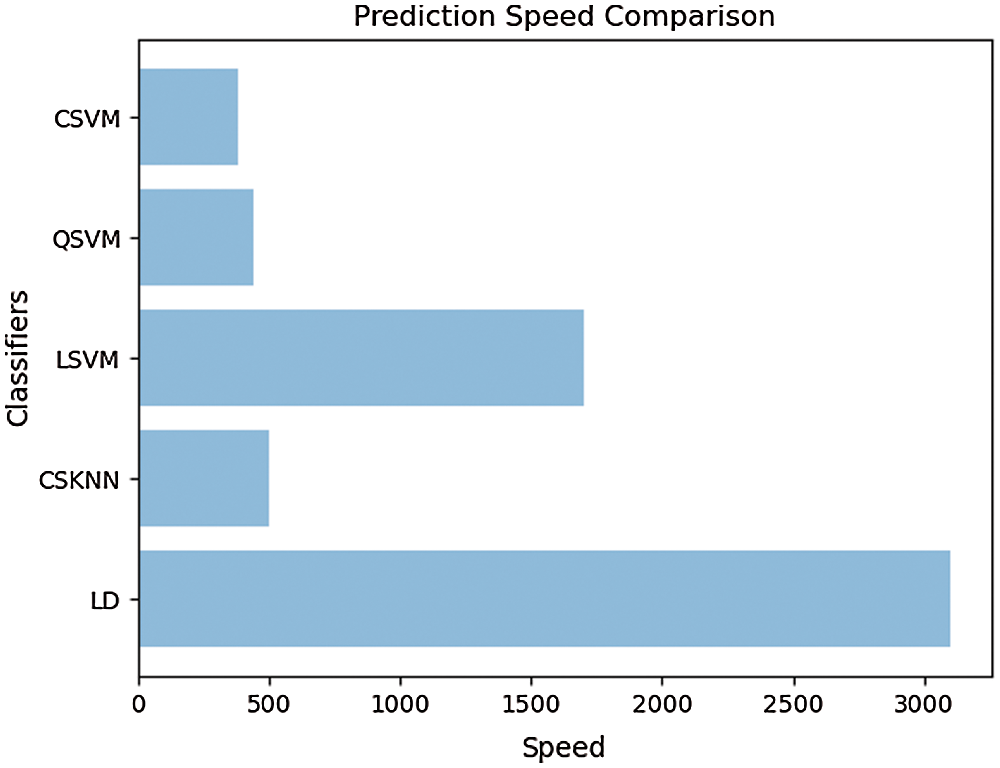
Figure 10: Prediction speed comparison between classifiers
Fig. 11. Shows the comparison based on accuracy results, training time, and prediction speed among various classifiers used. This gives a fair idea that some classifiers are better in prediction speed but compromise in providing better accuracy, whereas other do the reverse. CSVM is the only classifier that maintains the balance of everything by providing the best accuracy results and also maintaining an efficient training time and prediction speed. Tab. 5, shows the comparison of the proposed work with state of the arts. The proposed model excels from previous contributions in terms of accuracy and speed. Tab. 6 shows the comparison of proposed work with existing and latest works. The proposed model outperforms others in terms of accuracy and time consumption.
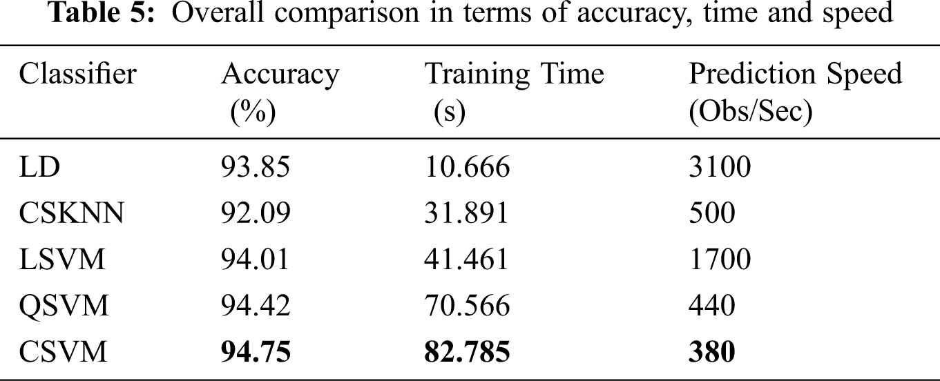
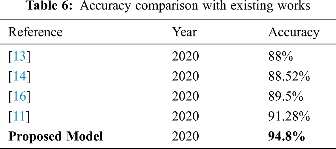
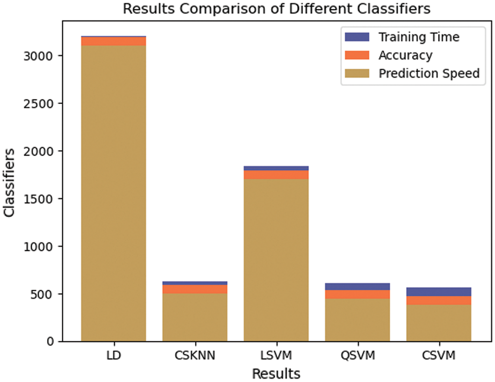
Figure 11: Prediction speed and training time comparison between classifiers
It is evident from the results reported above that when eight separate classifiers were implemented on the selected number of features derived from PSO, some contrasting results were achieved in terms of accuracy, training time, and prediction speed. We aim to conclude a classifier which when merged with the proposed model, provides a better balance of all the mentioned parameters. In this case, C-SVM is a classifier that provides the best accuracy of 94.8% while maintaining an optimal speed to time ratio. Therefore, C-SVM is chosen as the finalized classifier for our architecture. The proposed model stands out from all the previous works in terms of accuracy, time, and speed.
Vehicle classification is a challenging problem in the vast field of image classification. An autonomous and compact vehicle classification system can help in various tasks such as security, traffic analysis, and self-driving. In the proposed work, a PSO based deep learning model is proposed for classifying eight different types of vehicles. Data augmentation and filtering steps are performed before the images are passed on to the CNN GoogleNet, which performs feature learning and extraction. The features are optimized and reduced using the PSO algorithm. The selected features are finally tested and classified using a different set of classifiers. The CSVM classifier provides the best balance of accuracy, speed, and time consumption and outperforms the previous approaches.
Data Availability: The dataset used in this work is publicly available at Kaggle and can be accessed at “https://www.kaggle.com/iamsandeepprasad/vehicle-data-set”.
Funding Statement: This project was supported by the Deanship of Scientific Research at Prince Sattam Bin Abdulaziz University, Saudi Arabia under the research project # 2020/01/14224.
Conflicts of Interest: The authors declare that there is no conflict of interest regarding the publication of this paper.
1. Y. Zhou, H. Nejati, T. T. Do, N. M. Cheung and L. Cheah, “Image-based vehicle analysis using deep neural network,” A systematic study, in 2016 IEEE Int. Conf. on Digital Signal Processing (DSPBeijing, China, pp. 276–280, 2016. [Google Scholar]
2. X. Yu and P. D. Prevedouros, “Performance and challenges in utilizing non-intrusive sensors for traffic data collection,” Advances in Remote Sensing, vol. 2, no. 2, pp. 45–50, 2013. [Google Scholar]
3. L. Nanni, S. Ghidoni and S. J. P. R. Brahnam, “Handcrafted vs. non-handcrafted features for computer vision classification,” Pattern Recognition, vol. 71, pp. 158–172, 2017. [Google Scholar]
4. K. Makantasis, K. Karantzalos, A. Doulamis and N. Doulamis, “Deep supervised learning for hyperspectral data classification through convolutional neural networks,” in 2015 IEEE Int. Geoscience and Remote Sensing Sym. (IGARSSMilan, Italy, pp. 4959–4962, 2015. [Google Scholar]
5. Y. Gao, S. Guo, K. Huang, J. Chen, Q. Gong et al., “Scale optimization for full-image-CNN vehicle detection,” in 2017 IEEE Intelligent Vehicles Sym. (IVLos Angeles, CA, USA, pp. 785–791, 2017. [Google Scholar]
6. D. Weimer, B. Reiter and M. Shpitalni, “Design of deep convolutional neural network architectures for automated feature extraction in industrial inspection,” CIRP Annals, vol. 65, no. 1, pp. 417–420, 2016. [Google Scholar]
7. C. Wang, D. Yogatama, A. Coates, T. Han, A. Hannun et al., “Lookahead convolution layer for unidirectional recurrent neural networks,” ICLR 2016 Workshop, 2016. [Google Scholar]
8. J. Ryu, M. H. Yang and J. Lim, “Dft-based transformation invariant pooling layer for visual classification,” in Proc. of the European Conf. on Computer Vision (ECCVpp. 84–99, 2018. [Google Scholar]
9. F. Agostinelli, M. Hoffman, P. Sadowski and P. Baldi, “Learning activation functions to improve deep neural networks,” arXiv preprint arXiv:1412.6830, 2014. [Google Scholar]
10. W. Ma and J. Lu, “An equivalence of fully connected layer and convolutional layer,” arXiv preprint arXiv: 1712. 0152, 2017. [Google Scholar]
11. L. Lu, P. Wang and H. Huang, “A Large-Scale frontal vehicle image dataset for fine-grained vehicle categorization,” IEEE Transactions on Intelligent Transportation Systems, 2020. [Google Scholar]
12. J. J. Castro, J. C. Quiñonez, L. R. Hernández, G. Galaviz, D. Balbuena et al., “A Lean Convolutional Neural Network for Vehicle Classification,” in 2020 IEEE 29th Int. Sym. on Industrial Electronics (ISIEDelft, Netherlands, pp. 1365–1369, 2020. [Google Scholar]
13. C. M. García, W. F. Fuentes, D. H. Balbuena, J. C. R. Quiñonez, O. Sergiyenko et al., “Classification of Vehicle Images through Deep Neural Networks for Camera View Position Selection,” in 2020 IEEE 29th Int. Sym. on Industrial Electronics (ISIEDelft, Netherlands, pp. 1376–1380, 2020. [Google Scholar]
14. F. C. Soon, H. Y. Khaw, J. H. Chuah and J. Kanesan, “Semisupervised PCA convolutional network for vehicle type classification,” IEEE Transactions on Vehicular Technology, vol. 69, no. 8, pp. 8267–8877, 2020. [Google Scholar]
15. V. Sowmya and R. Radha, “Efficiency-optimized approach-vehicle classification features transfer learning and data augmentation utilizing deep convolutional neural networks,” International Journal of Applied Engineering Research, vol. 15, no. 4, pp. 372–376, 2020. [Google Scholar]
16. R. Dehkordi and H. Khosravi, “Vehicle type recognition based on dimension estimation and bag of word classification,” Journal of AI and Data Mining, vol. 8, no. 3, pp. 427–438, 2020. [Google Scholar]
17. S. Dabiri, N. Marković, K. Heaslip and C. Reddy, “A deep convolutional neural network based approach for vehicle classification using large-scale GPS trajectory data,” Transportation Research Part C: Emerging Technologies, vol. 116, pp. 102644, 2020. [Google Scholar]
18. MathWorks, “GoogleNet convolutional neural network,” 2020. [Google Scholar]
19. N. Kasim, N. Mat, N. Rahman, Z. Ibrahim and N. Mangshor, “Celebrity face recognition using deep learning,” Indonesian Journal of Electrical Engineering and Computer Science, vol. 12, no. 2, pp. 476–481, 2018. [Google Scholar]
20. J. Kennedy and R. Eberhart, “Particle swarm optimization,” Proceedings of ICNN’95-Int. Conf. on Neural Networks, vol. 4, pp. 1942–1948, 1995. [Google Scholar]
21. R. Poli, J. Kennedy and T. Blackwell, “Particle swarm optimization,” Swarm Intelligence, vol. 1, no. 1, pp. 33–57, 2007. [Google Scholar]
22. Y. Shi, “Particle swarm optimization: Developments, applications and resources,” Proceedings of the 2001 congress on evolutionary computation (IEEE Cat. No. 01TH8546), vol. 1, pp. 81–86, 2001. [Google Scholar]
 | This work is licensed under a Creative Commons Attribution 4.0 International License, which permits unrestricted use, distribution, and reproduction in any medium, provided the original work is properly cited. |