Computer Systems Science & Engineering DOI:10.32604/csse.2022.017744
Article

Model of a Composite Energy Storage System for Urban Rail Trains

Liang Jin1,*, Qinghui Meng1 and Shuang Liang2

1Department of Mechanical and Electrical, Henan Polytechnic Institute, Nanyang, 473000, China
2University of Florence, Firenze, 50041, Italy
*Corresponding Author: Liang Jin. Email: 19530521@163.com
Received: 09 February 2021; Accepted: 09 April 2021

Abstract: Urban rail transit can solve the current inconvenient transportation problem for China’s large urban population. A compound onboard energy storage system can meet vehicles’ traction requirements and recover energy in vehicles’ braking stage to improve energy utilisation. However, the composite onboard energy storage system has several concerns, such as its power and energy demand, battery aging, and maintenance costs. Therefore, the NSGA-II algorithm is proposed to optimise matching the composite energy storage system parameters for urban rail trains.

The NSGA-II algorithm was used with an improved elite retention strategy to optimise the parameters matching of the composite power supply. The optimisation’s objective concerns the replacement costs and economy of the composite power supply. The method increases the vertical diversity of searching and avoids genetic precocity. The NSGA-II algorithm calls the simulation model of composite power supply in real-time and simultaneously optimises the composite power supply and control parameters. The Pareto set of optimisation objectives and corresponding parameters and control strategies of composite power supply are obtained. The NSGA-II algorithm can optimise the composite energy storage system’s parameters and improve the train and the composite power supply’s performance indexes. The algorithm greatly reduces the composite power supply’s capacitance and reduces the system’s total energy consumption. Then, the multi-component energy loss caused by the multi-power source system can be effectively controlled. The total capacitance is reduced by 12.1%, the battery life is prolonged by 18.86%, and the optimised composite power supply’s energy storage is increased by 17.6%.

Keywords: Manuscript; preparation; typeset; format

1  Introduction

The goal of optimising the urban rail composite energy storage system is to reduce fuel consumption and emissions to meet the dynamic performance and performance constraints of its components. These characteristics are related to the parameters of the components of the power system. They are also affected by the control strategy’s parameters. This is a nonlinear and complex coupling relationship between the main components of the system. Therefore, there are still phases between the objective functions [1–3]. This paper addresses dealing with the multi-objective conflict problem and achieving the best overall performance.

The main methods of solving complex constrained nonlinear multi-objective optimisation problems can be divided into two categories: gradient-based and non-gradient-based. Gradient-based optimisation methods, such as sequential quadratic programming (SQP), assume that the objective function is continuous and differentiates and satisfies the Lipchitz condition [2–6]. The composite energy storage system is a complex nonlinear system. Its genetic algorithm has been widely used in multi-objective optimisation. It has also been applied in the parameter optimisation of hybrid electric vehicle components. However, it is rarely used in urban rail trains, which is worth studying [7–10].

However, current research has mainly solved this multi-objective problem by setting weights for different objective functions. This method can simplify the problem to some extent. However, it is challenging to determine the weights that are in line with the actual situation. The applied multi-objective genetic algorithm uses the non-dominant sorting method to deal with multiple objective functions, which can reduce oil consumption. The Pareto optimal solution set of this kind of integrated optimisation problem can be obtained by optimising the control strategy parameters with both consumption and emission as the optimisation objectives. This solution can provide various options for setting control strategy parameters [11–15].

2  Multi Objective Genetic Algorithm

2.1 Multi Objective Optimisation

There are often design and decision-making problems in engineering under multiple criteria or multiple design objectives [16]. If these objectives conflict, it is necessary to find the best design scheme to meet these objectives. The general expression of the multi-objective optimisation problem is as follows:

minf1(x1,x2,⋯,.xn)⋯⋯⋯⋯minfr(x1,x2,⋯,xn)maxfr+1(x1,x2,⋯,xn)⋯⋯⋯⋯maxfm(x1,x2,⋯,xn)s.t.gi(x)≥0,i=1,2,⋯,phj(x)=0,i=1,2,⋯,q (1)

Among them, f(x) is a multi-objective function, whereas gi(x)≥0 , hj(x)=0 is a set of constraints. The common method to solve the multi-objective optimisation problem is to transform the multi-objective into a single objective for optimisation. Common methods are the objective weighting method, hierarchical optimisation method, ε —constraint method, global quasi measurement method and objective planning method. There are often conflicts in the optimisation problem among the sub-objectives. Improving one sub-objective performance index will degrade the other sub-objective performance. Therefore, there is usually no optimal solution for all the objective functions simultaneously. French economist Pareto [17] first studied the multi-objective optimisation problem in economics and developed the Pareto optimality Theory. The multi-objective optimisation problem needs to optimise a set of functions whose solution is a set of points [18–20], called the Pareto optimal set. The Pareto optimal solution definition is as follows:

To minimise multi-objective problems, n objective components fk(k=1,...,n) can make of the vector f(x)=(f1(x),f2(x),...,fn(x)) f (x) = (F1 (x), F2 (x), … FN (x)), where xu∈U is the decision variable, and if xu is the Pareto optimal solution. It is satisfied if there is no variable xv∈U , v=f(xv)=(v1,v2,...,vn) dominates u=f(xu)=(u1,u2,...,un) . In other words, there is no xv∈U , which makes the following formula hold:

∀i∈{1,2,...,n},vi≤ui∧∃i∈{1,2,...,n},vi<ui (2)

In general, a multi-objective optimisation problem has multiple Pareto optimal solutions. The set of these solutions becomes the Pareto optimal solution set. The key to the multi-objective optimisation problem is to solve the Pareto optimal solution set. Fig. 1 shows a double objective unconstrained minimisation problem. The shadow part is the solution space. Notably, “R” is not the optimal solution, and point “C” is smaller than “R” in both objectives. Not all the solutions on the boundary “ABC” are optimal in the shadow. Still, all the solutions on the curve “ABC” are optimal, Pareto solutions.

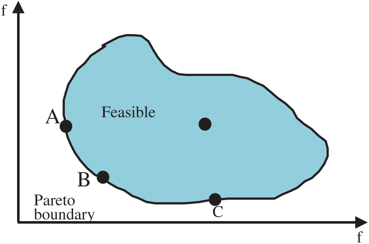
Figure 1: Pareto boundary diagram

2.2 Fast Non-Dominated Sorting Method

The non-dominated sorting method is used in the NSGA algorithm. The computational complexity of this method is O( mN3 ). Meanwhile, the computational complexity of the fast non-dominated sorting method is only O( mN3 ) in the NSGA-II algorithm. The following briefly explains the origin of the computational complexity of the two:

2.2.1 Computational Complexity of Non-Dominated Sorting Algorithm

Each individual must be compared with other individuals in the population to rank the population with m number and N size and determine whether the individual is dominated. In this way, each individual needs a total of mN times of comparison and O( mN ) calculation complexity. When this step is completed, continue to find all the individuals on the first non-dominated layer, which needs to traverse the entire population and have a total computational complexity of O( mN2 ). In this step, all the individuals in the first non-dominated layer are found. The previous operation is repeated to find the individuals in the subsequent levels. In the worst case (one individual at each level), all individuals of the whole population are graded. The computational complexity of this algorithm is O( mN3 ).

2.2.2 Computational Complexity of Fast Non-Dominated Sorting Algorithm

For each individual i in the population, there are two parameters: ni and Si . ni is the number of individuals who dominate the individual solution and Si is the set of individuals who are dominated by the individual solution.

(1) find all the individuals ni=0 in the population and store them in the current non-dominated set Z1 ;

(2) for each individual j in the current non-dominated set Z1 , traverse the set Sj of individuals it controls. Following this, subtract 1 from each individual in the set Sj . In other words, the solution’s number of individuals of the dominated individual t is nt reduced by 1 since the individual j of the dominated individual t was stored in the current non-dominated set Z1 . If nt−1=0 , the individual t is stored in another set H;

(3) as a set Z1 of first-order non-dominated individuals, the solution for the individuals is optimal. It only dominates the individual, but not any other individual. It assigns the same non-dominating order to all the individuals in the set ranki . Then, it continues to perform the above classification operation on the set Z1 . It also assigns the corresponding non-dominating order until all the individuals are classified. In other words, all individuals are assigned the corresponding non-dominating order.

Each iterative of operations (1) and (2) of the above fast non-dominated sorting algorithm steps requires N calculations. Therefore, the computational complexity of the whole iterative process is the largest. Therefore, the computational complexity of the whole fast non-dominated sorting algorithm is as follows: max(mN2,N2)=mN2

2.2.3 Congestion Determination

In the original NSGA algorithm, the shared niche technology is used to ensure the population’s diversity population [21,22]. However, the decision-maker needs to specify the value of the shared parameter shareσ . The crowding degree concept is quoted in NSGA-II to overcome this deficiency in the NSGA algorithm. The crowding degree refers to the density of individuals around a given point in the population, expressed by id , intuitively expressed by the length of the largest rectangle containing individuals but excluding other individuals around the individuals, as shown in Fig. 2.

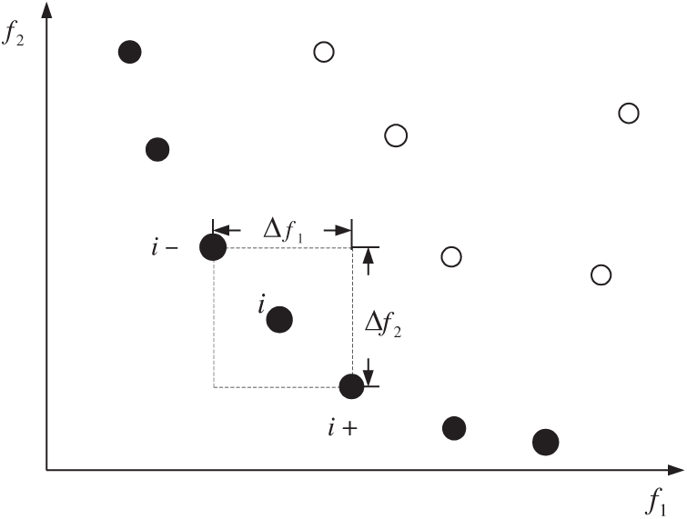
Figure 2: Individual crowding degree

In the non-dominated sorting genetic algorithm (NSGA-II) with an elite strategy, the crowding degree’s calculation is an important factor to ensure the population’s diversity. The calculation steps are as follows:

(1) the crowding degree id of each point is set to O;

(2) the population is non-dominated for each optimisation objective, and the crowding degree of two individuals on the boundary is infinite od=ld=∞ ;

(3) calculate the crowding degree of other individuals in the population:

id=∑j=1m(|fji+1−fji−1|) (3)

In the above formula, id represents the crowding degree of point i, fji+1 is the function value of the j objective function of point i+1, and fji−1 is the function value of the j objective function of point i-1.

2.2.4 Elite Strategy

The NSGA-II algorithm introduces the elite strategy to prevent losing excellent individuals in the process of population evolution. By mixing the parent population and the offspring population, non-dominated sorting can better avoid the loss of excellent individuals in the parent population. The execution steps of the elite strategy are shown in Fig. 3:

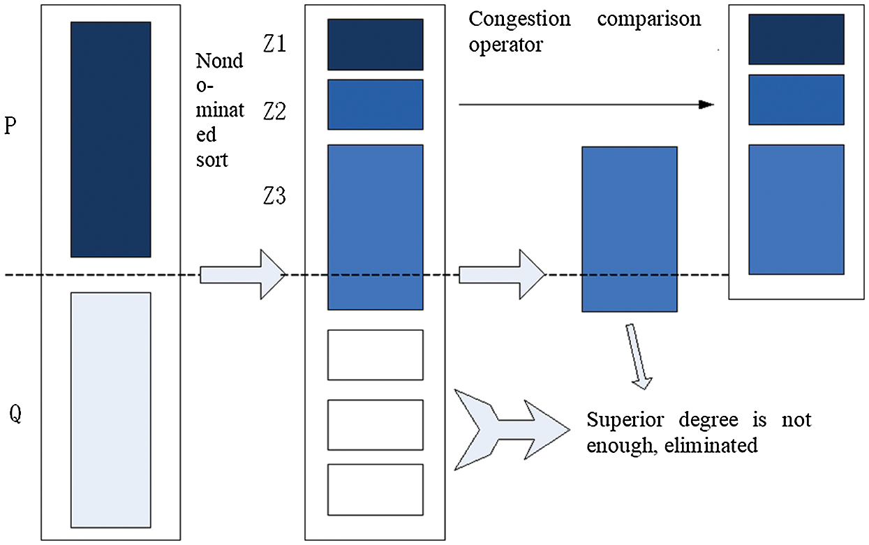
Figure 3: Execution steps of elite strategy

First, the offspring population Qt of the t generation and the parent population Pt should be combined to form a new species group Rt with the population size of 2N. Then, population Rt is arranged in the non-dominated order, a series of non-dominated sets Zi are obtained, and the crowding degree of each individual is calculated. Because the individuals of both parents and children are included in population Rt , the individuals included in the non-dominated set Z1 after non-dominated sorting are the best set of individuals Zi in the whole population Z1 . Therefore, the population will be put into the new parent population Pt+1 . If the size of population Pt+1 is smaller than N at this time, it is necessary to continue to add the next level of the non-dominated set Z2 to population Pt+1 until the size of the population exceeds that of the non-dominated set Zn . Following this, the crowding degree comparison operator is used for each individual in the population. The first individual is taken {num(Zn)−(num(Pt+1)−N)} to make the population reach the size. Then, the new offspring population Qt+1 is generated through genetic operators, such as selection, crossover and mutation.

In the NSGA-II algorithm, a congestion comparison operator is introduced to ensure the diversity of non-inferior solutions. The crowding degrees of all individuals in the population are compared. Therefore, there is no dependence on the shared parameters shareσ in the NSGA algorithm in this process.

3  Simulation Results

In this paper, the experimental environment parameters are as follows: the population size is 100, the default evolution algebra is 100, the mating pool size is 50, the crossover probability is 0.9, the mutation probability is 0.1, the probability level is 0, the weight coefficient is 1, the regularisation factors are 1.05 and 1, the uncertainty level of determined parameters is, and the penalty factor is 1000. The calculation results in this paper are as follows in the Figs. 4–6.

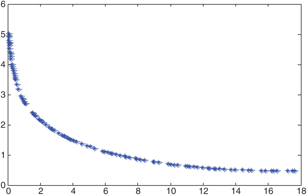
Figure 4: Simulation results

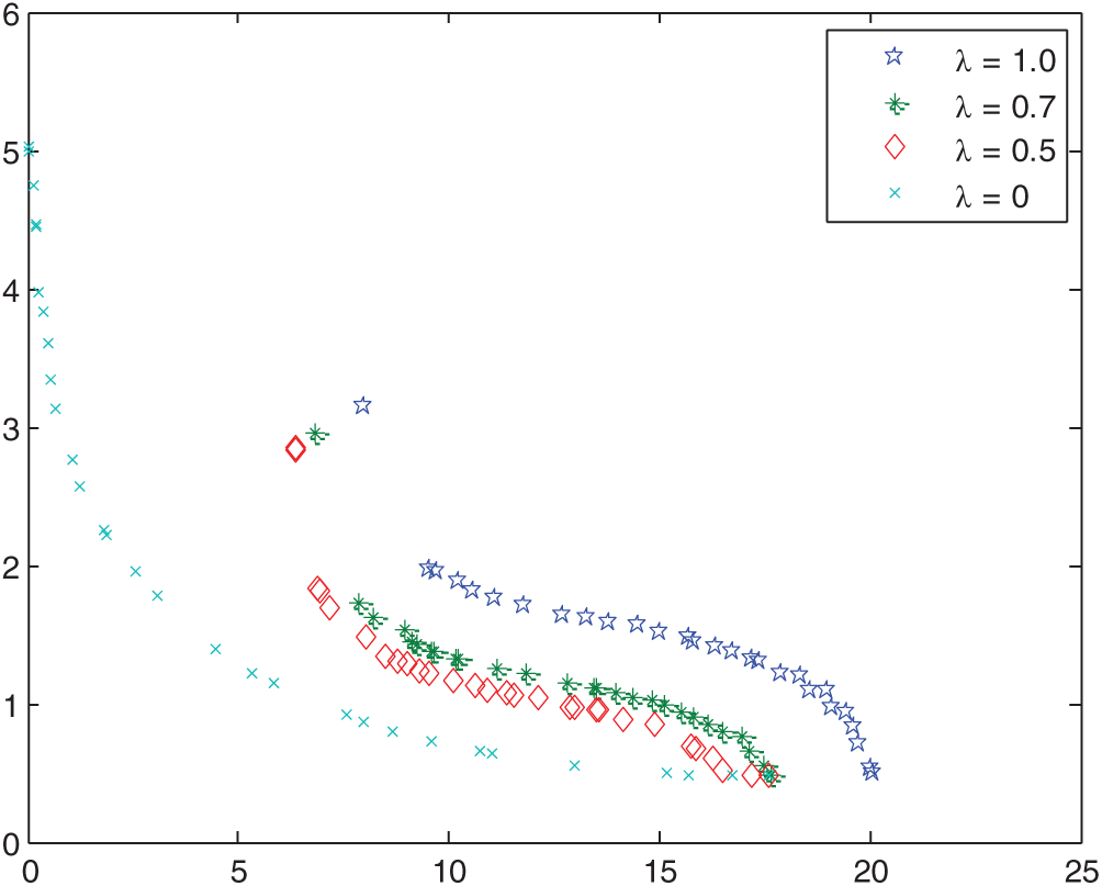
Figure 5: Pareto front under different constraint probability levels λ

Figure 6: Pareto front under different multi-objective weight coefficients β

(1) The influence of constraint probability level λ

Generally, the interval uncertainty constraints can be satisfied at a certain level of possibility in interval number optimisation. Then, uncertainty constraints can be transformed into deterministic constraints. Therefore, selecting the probability level affects the distribution of non-inferior solutions directly and plays a key role in the final optimisation results. In this section, we will discuss the Pareto frontier under different probability values. We will further explain the probability value’s influence on the final optimisation results by analysing the final MATLAB simulation results. The following is the Pareto front in the case of the weight coefficient β = 1. The probability level values are λ = 0, λ = 0.5, λ = 0.7, λ = 1.0, respectively which is shown in the Fig. 5.

(2) The selection of the multi-objective weight coefficient β

This section will discuss the optimisation results of the same objective function under different values of the multi-objective weight coefficient β. Following this, it will determine the influence of the multi-objective weight coefficient β on the final optimisation results. The following is a list of the final optimisation results when the multi-objective weight coefficient β = 0, β = 0.5, β = 0.7 and β = 1.0 at the possibility level λ = 0 in the Fig. 6.

4  Conclusions

The NSGA-II algorithm is used to solve the multi-objective joint optimisation problem of the composite energy storage system. The algorithm aims to improve vehicles’ economy and the replacement costs of the composite energy storage system. The algorithm can call the working condition model of the composite energy storage system in real-time and read the simulation results for further processing. According to the Pareto set of the two objective values obtained by the algorithm, the initial cost, average daily cost and battery life mileage of each solution in the Pareto set are further compared and optimised. The final solution is obtained. The final matching parameters significantly reduce the composite energy storage system’s replacement costs without reducing the whole vehicle’s economy. At the same time, the initial cost and other indicators also achieve satisfactory results.

Acknowledgement: We thank the team members for their hard work, the scientific research platform provided by the University, and the strong support from government funds.

Funding Statement: This work was supported by Henan province’s project of science and technology under Grant No. 202102210134.

Conflicts of Interest: The authors declare that they have no conflicts of interest to report regarding the present study.

References

 1.  T. He and R. Q. Xiong, “Research on multi-objective real-time optimization of automatic train operation (ATO) in urban rail transit,” Journal of Shanghai Jiaotong University (Science), vol. 23, no. 2, pp. 121–129, 2015. [Google Scholar]

 2.  Z. Chen, B. Mao and Y. Bai, “Optimization on energy-efficient operations for trailing train in urban rail system with fixed run-time,” Journal of the China Railway Society, vol. 39, no. 8, pp. 10–17, 2017. [Google Scholar]

 3.  H. Li, J. Peng and J. Wang, “An adaptive parallel charging system for energy-storage urban rails,” Proceedings of the American Control Conf., vol. 24, no. 5, pp. 1573–1578, 2015. [Google Scholar]

 4.  S. J. Li, R. H. Xu and K. Han, “Demand-oriented train services optimization for a congested urban rail line: Integrating short turning and heterogeneous headways,” Transportmetrica A: Transport Science, vol. 18, no. 6, pp. 1–35, 2019. [Google Scholar]

 5.  B. James and Y. Bengio, “Random search for hyper-parameter optimization,” Journal of Machine Learning Research, vol. 13, no. 1, pp. 281–305, 2012. [Google Scholar]

 6.  Y. H. Li, X. M. Lu and C. Narayan, “Rule-Based control strategy with novel parameters optimization using NSGA-II for Power-Split PHEV operation cost minimization,” IEEE Transactions on Vehicular Technology, vol. 63, no. 7, pp. 3051–3061, 2015. [Google Scholar]

 7.  T. Y. Lin, L. B. Qiao and T. Zhang, “Stochastic primal-dual proximal extragradient descent for compositely regularized optimization,” Neurocomputing, vol. 15, no. 12, pp. 254–268, 2017. [Google Scholar]

 8.  J. Su, Z. Sheng, A. X. Liu and Y. Chen, “A partitioning approach to RFID identification,” IEEE/ACM Transactions on Networking, vol. 28, no. 5, pp. 2160–2173, 2020. [Google Scholar]

 9.  J. Su, Z. Sheng, A. X. Liu, Y. Han, Y. Chen et al., “Capture-aware identification of mobile RFID tags with unreliable channels,” IEEE Transactions on Mobile Computing, vol. 56, no. 12, pp. 1–14, 2020. [Google Scholar]

10. X. Zhao, X. Wang and H. Sun, “A self-adaptive differential evolution algorithm with an external archive for unconstrained optimization problems,” Journal of Intelligent & Fuzzy Systems, vol. 29, no. 5, pp. 2193–2204, 2015. [Google Scholar]

11. V. Pombo and J. Murta-Pina, “Distributed energy resources network connection considering reliability optimization using a NSGA-II algorithm,” in 11th IEEE Int. Conf. on Compatibility, Cadiz, Spain, pp. 631–642, 2017. [Google Scholar]

12. A. Y. Hamed, M. H. Alkinani and M. R. Hassan, “A genetic algorithm to solve capacity assignment problem in a flow network,” Computers Materials & Continua, vol. 64, no. 3, pp. 1579–1586, 2020. [Google Scholar]

13. S. G. Nair and N. Senroy, “Parameter optimization and sizing of flywheel energy storage system,” in IEEE Recent Advances in Intelligent Computational Systems. Trivandrum, Kerala, India, pp. 1325–1331, 2015. [Google Scholar]

14. F. Chou, W. Ho and C. Chen, “Niche genetic algorithm for solving multiplicity problems in genetic association studies,” Intelligent Automation & Soft Computing, vol. 26, no. 3, pp. 501–512, 2020. [Google Scholar]

15. Y. Huang, X. Chen, K. Yuan, J. Zhang and B. Liu, “Directional modulation based on a quantum genetic algorithm for a multiple-reflection model,” Computers Materials & Continua, vol. 64, no. 3, pp. 1771–1783, 2020. [Google Scholar]

16. J. Su, R. Xu, S. Yu, B. Wang and J. Wang, “Idle slots skipped mechanism based tag identification algorithm with enhanced collision detection,” KSII Transactions on Internet and Information Systems, vol. 14, no. 5, pp. 2294–2309, 2020. [Google Scholar]

17. L. Li, L. Sun, J. Guo, S. Li and P. Jiang, “Identification of crop diseases based on improved genetic algorithm and extreme learning machine,” Computers Materials & Continua, vol. 65, no. 1, pp. 761–775, 2020. [Google Scholar]

18. J. Su, R. Xu, S. Yu, B. Wang and J. Wang, “Redundant rule detection for software defined networking,” KSII Transactions on Internet and Information Systems, vol. 14, no. 6, pp. 2735–2751, 2020. [Google Scholar]

19. A. Alhroob, W. Alzyadat, A. T. Imam and G. M. Jaradat, “The genetic algorithm and binary search technique in the program path coverage for improving software testing using big data,” Intelligent Automation & Soft Computing, vol. 26, no. 4, pp. 725–733, 2020. [Google Scholar]

20. S. Abed, M. H. Ali and M. Al-Shayeji, “Enhanced GPU-based anti-noise hybrid edge detection method,” Computer Systems Science and Engineering, vol. 35, no. 1, pp. 21–37, 2020. [Google Scholar]

21. A. Y. Hamed, M. H. Alkinani and M. R. Hassan, “A genetic algorithm optimization for multi-objective multicast routing,” Intelligent Automation & Soft Computing, vol. 26, no. 6, pp. 1201–1216, 2020. [Google Scholar]

22. R. Saraçoğlu and A. F. Kazankaya, “Developing an adaptation process for real-coded genetic algorithms,” Computer Systems Science and Engineering, vol. 35, no. 1, pp. 13–19, 2020. [Google Scholar]

This work is licensed under a Creative Commons Attribution 4.0 International License, which permits unrestricted use, distribution, and reproduction in any medium, provided the original work is properly cited.