Computer Systems Science & Engineering DOI:10.32604/csse.2022.018911
Article

FPD Net: Feature Pyramid DehazeNet

Shengchun Wang1, Peiqi Chen1, Jingui Huang1,* and Tsz Ho Wong2

1College of Information Science and Engineering, Hunan Normal University, Changsha, 410081, China
2Blackmagic Design, Rowville, VIC, 3178, Australia
*Corresponding Author: Jingui Huang. Email: hjg@hunnu.edu.cn
Received: 25 March 2021; Accepted: 08 May 2021

Abstract: We propose an end-to-end dehazing model based on deep learning (CNN network) and uses the dehazing model re-proposed by AOD-Net based on the atmospheric scattering model for dehazing. Compare to the previously proposed dehazing network, the dehazing model proposed in this paper make use of the FPN network structure in the field of target detection, and uses five feature maps of different sizes to better obtain features of different proportions and different sub-regions. A large amount of experimental data proves that the dehazing model proposed in this paper is superior to previous dehazing technologies in terms of PSNR, SSIM, and subjective visual quality. In addition, it achieved a good performance in speed by using EfficientNet B0 as a feature extractor. We find that only using high-level semantic features can not effectively obtain all the information in the image. The FPN structure used in this paper can effectively integrate the high-level semantics and the low-level semantics, and can better take into account the global and local features. The five feature maps with different sizes are not simply weighted and fused. In order to keep all their information, we put them all together and get the final features through decode layers. At the same time, we have done a comparative experiment between ResNet with FPN and EfficientNet with BiFPN. It is proved that EfficientNet with BiFPN can obtain image features more efficiently. Therefore, EfficientNet with BiFPN is chosen as our network feature extraction.

Keywords: Deep learning; dehazing; image restoration

1  Introduction

Due to the presence of turbid media in the atmosphere (e.g., dust, mist, smoke, and haze), the visibility of the images captured by the camera will be greatly affected, such as the loss of contrast and saturation, and the overall brightness of the image will be dark. This lack of clarity also has an adverse effect on the post-processing of the computer vision system, which interferes with the performance of the computer vision system. Therefore, we need clear images as input to the computer vision system.

Single image dehaze is an image recovery process that goes through an atmospheric scattering model to obtain clear images. However, it is difficult to solve because of the difficulty in estimating the atmospheric scattered light and transmission maps. Within the last few decades, a variety of different dehazing methods have been proposed to solve this problem. We can broadly classify them into two categories, including traditional prior-based methods [1–6] and deep learning-based methods [7–10]. The major difference between these methods is that the former is based on statistical prior information for dehazing and while the latter is self-adaptive dehazing through learning.

2  Related Work

2.1 Traditional Methods

In traditional prior-based methods, many different images of statistical prior information are used as additional constraints to compensate for the loss of information during corruption. Dark channel prior (DCP) improves the dark channel prior dehazing algorithm by computing the transmission matrix more efficiently [11,12]. Meng et al. [5] obtains clearer images through boundary constraints and contextual regularization. Color attenuation prior (CAP) is performed on blurred images to establish a linear model of scene depth, and then the model parameters are learned supervised. However, the dehazing performance of the above methods is not always satisfactory because of the physical parameters estimates for a single image which is often inaccurate.

2.2 Learning-based Methods

With the success of CNNs for advanced vision tasks such as image classification [13], target detection [14], and instance segmentation [15], attempts have been made to use CNNs to perform image dehaze. In deep learning-based dehazing methods, dehazing is often performed by estimating the transmission matrix, learning the mapping, and estimating the numerical gap between clear and hazy images. For example, Dehaze-Net deal with hazy images by estimating the transmission matrix, but an inaccurate estimation of the transmission map will reduce the model's dehazing effect. The method of using GAN network to denoise often uses a generator to generate a denoised image and a discriminator to judge the effect of denoising, such as [16]. AOD-Net uses a deformed atmospheric scattering model, which generalizes two unknowns in the atmospheric scattering model to a single unknown to reduce the loss in the dehazing process. AOD-Net uses a lightweight network to improve the speed of dehazing. However, there is a difference in effect compared with other networks. Instead of end-to-end dehazing and dehazing by estimating the transmission matrix, GCA-Net dehazes hazy images by estimating the difference between the clear image and the hazy image, which greatly improves the effect and quality of dehazing. Since GCA-Net uses ReLU [17] as an activation function in the network, the result obtained by GCA-Net is often positive, but in reality, a portion of the pixel difference between the clear and hazy images is negative, which prevents GCA-Net from fully estimating the difference between the clear and hazy images, resulting in an increase in loss.

2.3 Pyramid Structure

The pyramid structure has been widely used in various fields of computer vision. The spatial pyramid pooling methods [18–20] use different proportions to extract information from the context of the picture, thereby reducing the computational complexity. SPP-Net [21] introduces spatial pyramid pooling into CNN, which relieves the limitation of CNNs on the input image size. PSP-Net [22] performs spatial pooling on several different scales and has achieved excellent results in the direction of semantic segmentation. In the field of target detection, FPN [23] performs hierarchical prediction on high-level and low-level semantics [24]. The network proposed in this paper combines high-level and low-level semantics. Compared with the use of two networks in Chen et al. [25] to extract image features separately, FPN can effectively reduce the amount of calculation, and can make full use of the underlying features, thereby effectively obtaining global and local features.

2.4 Multi-scale Features in the Dehazing Network

Many dehazing networks use different methods to obtain multi-scale features of hazy images. Dehaze-Net uses convolution kernels of different sizes to try to obtain multi-scale features of the image. Similar to Dehaze-Net, AOD-Net uses 1×1 , 3×3 , 5×5 and 7×7 convolution kernels to obtain multi-scale features of the hazy image, and uses intermediate connections to connect features of different sizes to compensate for the loss of information in the convolution process. GCA-Net uses smoothed dilated convolution to solve the contradiction between the required multi-scale context inference and the spatial resolution information lost during downsampling. GCA-Net uses a method which is similar to FPN to obtain three different levels of feature maps, and then perform feature fusion through gated fusion subnets to obtain low-level and high-level semantic features of the image. Compared with the method of using different sizes of convolution kernels and smoothed dilated convolution, the feature extractor using FPN structure can obtain feature maps of different sizes more effectively and can effectively extract low-level and high-level semantic features of hazy images.

2.5 Main Contributions

In this paper, we propose a new dehazing method, FPD-Net. FPD-Net is inspired by the FPN structure in target detection and uses the FPN structure for feature extraction. The feature extractor of the FPN structure can take into account both global and local features well, and it is easier to obtain the comprehensive features of the image. Wang et al. [26] proposed a block dehazing, and matching the whole image uniformly does not have a good dehazing effect, so block dehazing is carried out according to the hazy level and then matched separately. In the feature extraction process of pictures, the receptive fields are different for different sizes of feature maps. For the neural network, the large-size feature map can better extract the detailed features, which is suitable for extracting the features of hazy images with a big difference in the concentration of regional haze, and the small-size feature map can better take into account the global features, which is suitable for extracting the features of haze images with a big difference in the concentration of regional haze. The FPD-Net uses the FPN structure as a feature extractor to obtain five feature maps with different sizes, and then the FPD-Net uses bilinear interpolation to make all the feature maps of the same size, and then fusion decoding by the convolutional neural network to obtain a composite feature. This process enables FPD-Net to synthesize the global and local features, and finally obtain a better dehazing result.

In this paper, the main contributions are in the following three areas:

This paper presents a new type of dehazing network, FPD-Net. FPD-Net uses the FPN network in the target detection domain as a feature extractor and uses different sized feature maps for dehazing to better obtain the features of the hazy image in different size regions.

The FPD-Net has been shown to achieve better qualitative and quantitative performance than all previous state-of-the-art image dehazing methods. At the same time, FPD-Net provides excellent performance in terms of speed and performance while maintaining the highest quality of dehazing.

FPD-Net adopts full convolutional structure and bilinear interpolation for up-sampling, there is no restriction on the size of the input picture, so you can input any size picture for dehazing, and keep the original size to output clear picture.

3  Method

In this section, we will first describe the dehazing model used by FPD-Net and then go on to describe the network structure of FPD-Net in detail. The network structure of FPD-Net is composed of two parts: the first part is to calculate k(x) based on the input hazy image, the second part is the physical model part, using the k(x) obtained by the first part to gets a clear image. The physical model in Eq. (3), and the network is shown in Fig. 1.

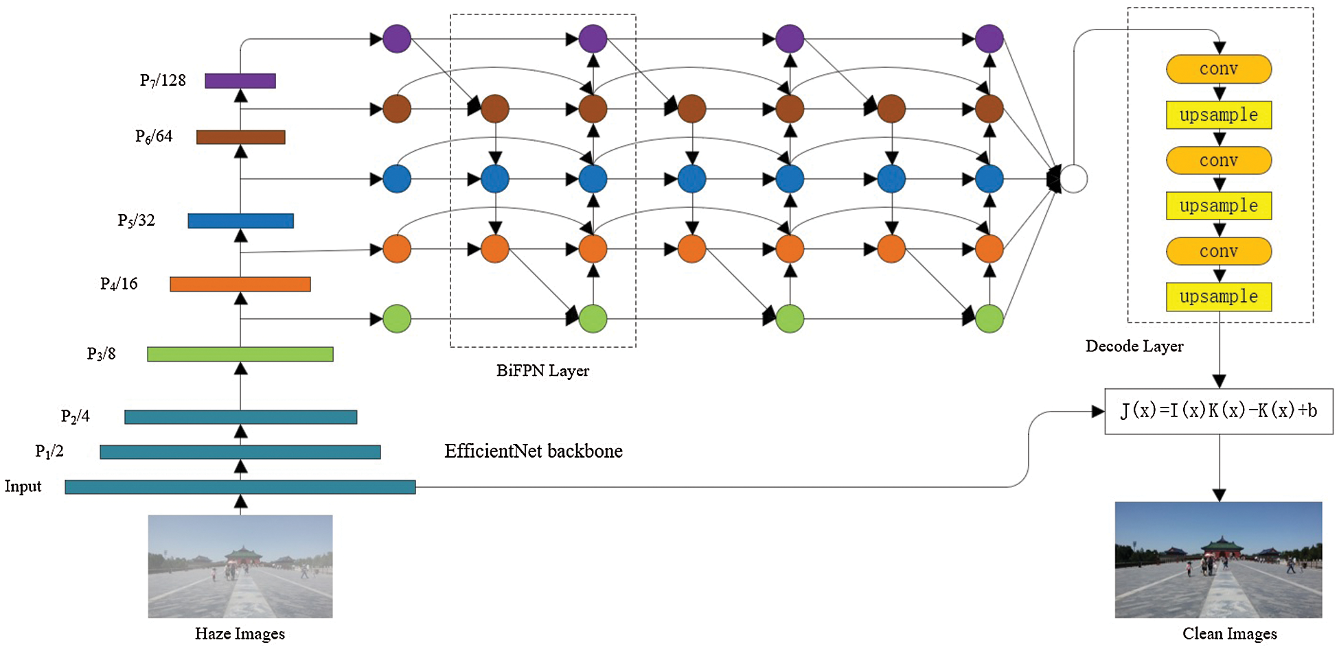
Figure 1: Network structure

3.1 Physical Model and Its Changing Formula

The generation of hazy images usually follows a physical model, the atmospheric scattering model [27–29]:

I(x)=J(x)t(x)+A(1−t(x)) (1)

where I(x) and J(x) denote the observable hazy image and the actual clear image respectively. A is the global atmospheric light, and t(x) denotes the transmission matrix. Many previous neural network-based dehazing methods estimate the transmission matrix t(x) or global atmospheric light A first, and finally, obtain clear images through the atmospheric scattering model. AOD-Net deforms the model according to the atmospheric scattering model, converting the model with two unknowns into a physical model with only one unknown, which can effectively reduce the loss due to the existence of two unknowns. The error introduced by two unknowns. In the following, we will present this model.

We can rewrite Eq. (1) to get the following formula:

J(x)=1t(x)I(x)−A1t(x)+A (2)

Convert Eq. (2) to get a physical model with only one unknown:

J(x)=k(x)I(x)−k(x)+b,where,k(x)=1t(x)(I(x)−A)+(A−b)I(x)−1 (3)

Thus, the original unknowns t(x) and A in Eq. (2) are integrated into the new variable k(x) , and b is a constant deviation with a default value of one. The resulting deformed physical model Eq. (3) contains only one unknown, which effectively reduces the bias introduced by the two unknowns.

3.2 FPN Feature Extraction Layer

For the feature extraction layer, we choose to use a network with strong feature extraction capability and high efficiency. Tan et al. [30] pointed out that EfficientNet compared to ResNet [31], DenseNet [32], ResNeXt [33], and SeNet [34], etc., while maintaining lightweight, it can have stronger feature extraction capabilities, so we choose to use EfficientNet serves as the backbone network. Tan et al. [35] compared with PA Net [36] and NAS-FPN [37], the proposed BiFPN has a smaller number of parameters and excellent performance. In this article, we will use Bi FPN. In this part, we also tried to use ResNet and FPN for feature extraction. With the continuous deepening of ResNet layers, the network's dehaze effect is better. We used gradient cropping in the training process. Gradient cropping can make the network dehazing effect using ResNet and FPN as a feature extractor better. Gradient cropping has been widely used in recurrent network training [38]. However, due to the relatively large ResNet network, the speed is slower than EfficientNet, and the effect of EfficientNet dehaze is better. When EfficientNet is used as the backbone network, the deeper network dehaze effect is better, but the training period and prediction time are longer, and the occupied video memory is also more. For comprehensive consideration, we chose EfficientNet-B0 and BiFPN as the feature extractor with better dehazing results, faster speed, and lighter network. We can see the comparison result of EfficientNet with BiFPN and ResNet with FPN in Fig. 2.

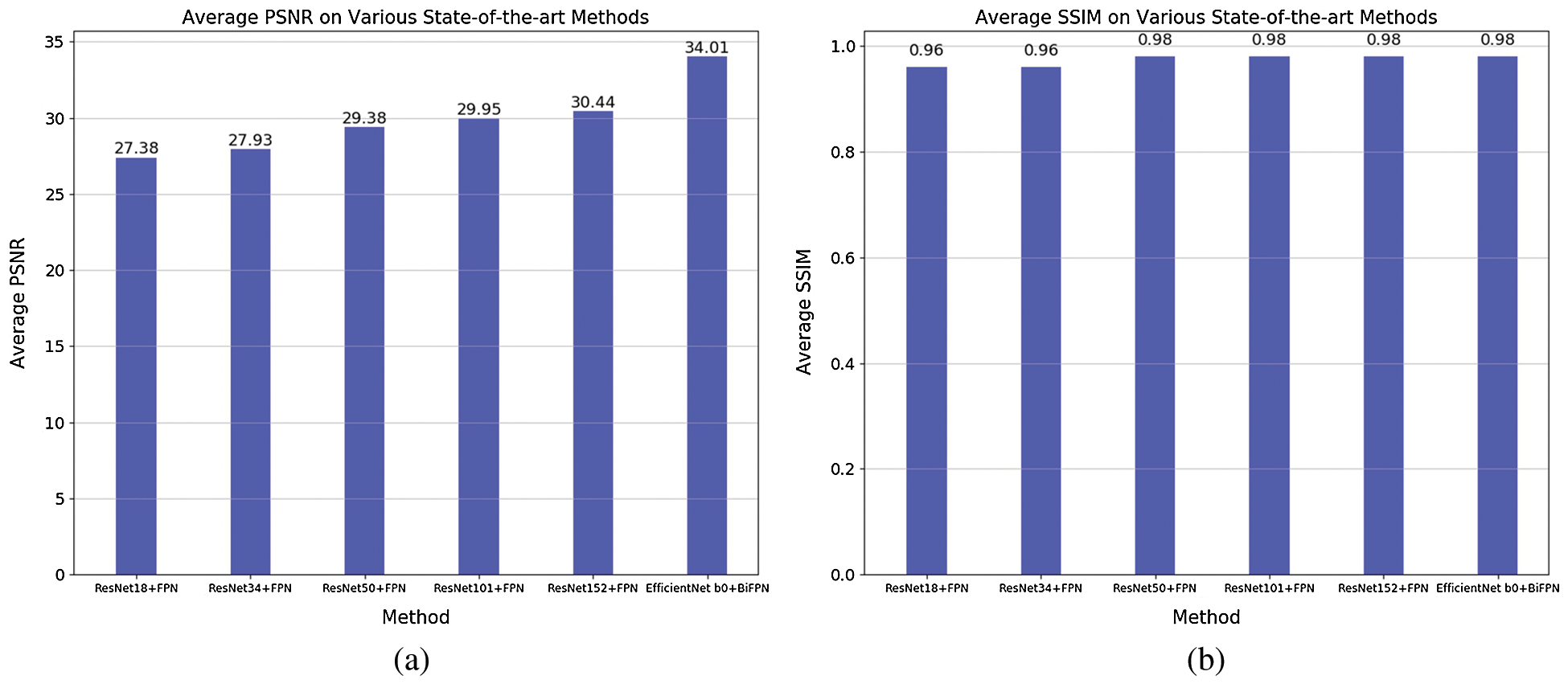
Figure 2: Comparison of EfficientNet with BiFPN and ResNet with FPN. (a) PSNR, (b) SSIM

ConvNet layer i can be defined as a function: Yi=Fi(Xi) , where Fi is the operation, Xi is the input data, and Yi is the output data. We can divide the convolutional layer of CNNs into multiple stages, and all layers of each stage have the same structure. For example, EfficientNet has 8 stages of convolution. Therefore, we can define the convolutional layer N of s stage CNNs as:

Ns=⊙i=1…s⁡FiLi(x⟨Hi,Wi,Ci⟩) (4)

where FiLi represents ConvNet layer i is repeated Li times in stage i , and ⟨Hi,Wi,Ci⟩ represents the shape of the input tensor X of the i layer. ⊙ represents the composition operator, which represents the composition of FsLs , Fs−1Ls−1 , …, F1L1 .

Tan et al. [30] scaled all layers at a constant ratio, and got the following formula:

Ns(d,w,r)=⊙i=1…sF^id·L^i(X〈r·H^i,r·W^i,r·C^i〉) (5)

where d , w , r are the coefficients used to scale the depth, width and resolution of the network, Fi^ , Li^ , Hi^ , Wi^ , Ci^ are predefined parameters in the baseline network.

Under the constraints of d⋅w2⋅r2≈2 , they found that Efficient-B0 has the best effect when d=1.2 , w=1.1 , and r=1.15 .

We use Efficient-B0 as the backbone network to get five feature maps of different sizes. Similar to Refs. [22,39], feature maps of different sizes are extracted, the purpose is to better obtain features of different proportions and different sub-regions.

P3,P4,P5,P6,P7=M(Ihaze) (6)

Pi=Conv(Ni+1(d=1.2,w=1.1,r=1.15)),i=3…7 (7)

where M represents the feature extraction operation of the backbone network, Ihaze represents the input haze image, Conv is used to represent the convolution operation, the number of channels of Pi is unified to 64 through Conv , and Ni+1 represents the backbone performs i convolutional layers stage.

Fast normalized fusion enables BiFPN to obtain very good results while maintaining fast calculations. The formula is as follows:

O=∑iwiε+∑jwj (8)

where wi is a learnable weight and 0≤wi≤1 , ε=0.0001 is a small value to ensure the stability of the value.

We express BiFPN as the following formula:

P3out,P4out,P5out,P6out,P7out=BiFPN(P3in,P4in,P5in,P6in,P7in) (9)

And the specific calculation of Piout(i=3,4,…,7) is as follows. Where Piin is the input feature, Pitd is the intermediate result, and Piout is the output feature. Resize is usually an up-sampling or down-sampling operation.

P3out=Conv(w1⋅P3in+w2⋅Resize(P4td)w1+w2+ε) (10)

Pitd=Conv(w1⋅Piin+w2⋅Resize(Pi+1td)w1+w2+ε),wherei=4,5 (11)

P6td=Conv(w1⋅P6in+w2⋅Resize(P7in)w1+w2+ε) (12)

Piout=Conv(w′1⋅Piin+w′2⋅Pitd+w′3⋅Resize(Pi−1out)w′1+w′2+w′3+ε),wherei=4,5,6 (13)

P7out=Conv(w1⋅P7in+w2⋅Resize(P6out)w1+w2+ε) (14)

P3 , P4 , …, P7 passes through three consecutive BiFPN layers to obtain new features P3out , P4out , …, P7out . Then we use the upsampling method of bilinear interpolation to make the five feature maps of different sizes consistent in size, and fuse the feature maps to obtain the fused feature FF:

FF=Conv(P3out+∑i=4…7Resize(Piout)) (15)

3.3 Decode Layer

Similarly to Refs. [40–43], we use a simple decoder to stitch five feature maps together for fusion decoding and finally obtain k(x) . The Decode layer is composed of three decode modules D:

D(FF)=upsample(Conv(FF)) (16)

where upsameple represents the up-sampling operation, and FF is the fusion feature obtained by the FPN feature extraction layer.

BiFPN can effectively obtain detailed information and global information and can obtain very good performance under a lightweight network structure. Using EfficientNet-B0 and BiFPN can achieve high-efficiency results while keeping the network lightweight. At the same time, this article changes the BiFPN upsampling process. BiFPN originally used the unpooling method, so the size of the input image needs to be limited, resulting in a reduction in a network application. In this paper, unpooling is changed to bilinear interpolation, so that small-size feature maps can be directly consistent with the size of the feature map to be fused through bilinear interpolation, so there is no need to limit the size of the input picture, which increases the network application scenes.

3.4 Clean Image Generation Module

In the second part, we use the dehazing model which was proposed by AOD-Net based on the atmospheric scattering model to compute the k(x) estimated in the first part in combination with the hazy picture to obtain the clear picture. Through repeated learning and training, FPD-Net is able to better learn the value of k(x) . This end-to-end learning can effectively avoid the tedious work and loss caused by the manual estimation of k(x) , and can learn k(x) more efficiently from the clear image, and finally obtain a dehazing model with good performance and speed.

3.5 Loss Function

In the previous dehaze network based on deep learning [44,45], a simple MSE loss is used, and the loss function used in this paper is also MSE Loss. MSE can effectively reflect the loss between the clear picture obtained by FPD-Net and the clear picture of the target and can be effectively propagated to the k(x) estimation module through Eq. (3). Finally, through continuous adjustment, k(x) can be estimated more accurately.

Loss=(Igt−Ipred)2 (17)

4  Experiments

4.1 Experimental Implementation Details

In the experiment, we verified the effectiveness of FPD-Net dehazing. We train and evaluate FPD-Net on public data sets, and compare the experimental results with previous methods. In the experiment, FPD-Net uses Adam optimizer to train 100 Epochs, the default initial learning rate is 0.0001, and then takes its best experimental result as the final result of the experiment. We used PyTorch [46] to conduct experiments on a GTX 1080ti graphics card.

4.2 Dataset Setup

We found that the data set used in the method proposed in many papers was synthesized according to the atmospheric scattering model of Eq. (1), and only this particular data set was evaluated. This method is not objective, so in this article, we use the dehaze evaluation data set RESIDE provided by Google. Its test set and training set are composed of a large number of depth and stereo data composition. Li et al. [47] used different evaluation indicators to evaluate the existing dehazing algorithms and compared them in more detail. Although the test data set of RESIDE includes indoor and outdoor images, they only report quantitative results for the indoor portion. According to their strategy, we also made a quantitative and qualitative comparison of the methods of indoor datasets and outdoor datasets. In addition to the pros and cons of the algorithm itself, the performance of the algorithm is still highly dependent on the data set, so we choose to use transfer learning to improve the performance of the algorithm. In addition to the pros and cons of the algorithm itself, the performance of the algorithm is still highly dependent on the data set, so we choose to use transfer learning to improve the performance of the algorithm [48].

4.3 Quantitative and Qualitative Evaluation for Image Dehazing

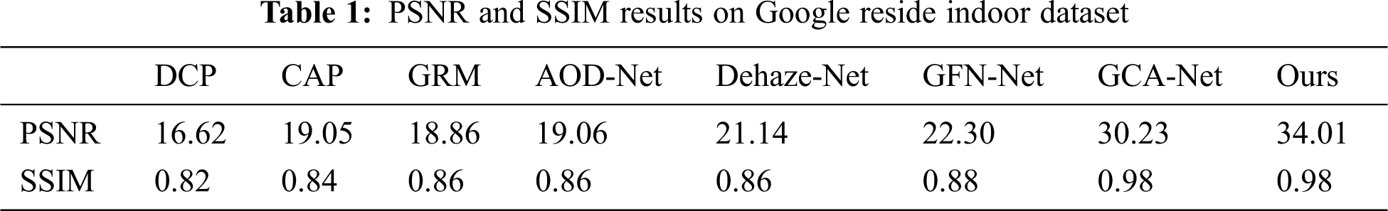
In this part, we compare FPD-Net with the previous dehaze methods from the quantitative and qualitative parts. We choose three traditional prior-based methods: DCP, CAP, and GRM, and four other deep learning-based dehazing methods: AOD-Net, Dehaze-Net, GFN-Net [49], and GCA-Net. Li et al. [47] proposed various evaluation indicators, but this paper still chooses PSNR and SSIM, the two most widely used indicators. For the convenience of comparison, other than GCA-Net, other experimental structures are directly quoted from Li et al. [47]. As shown in Tab. 1, FPD-Net is superior to the other seven methods in PSNR and SSIM. We show the dehazing effects on indoor hazy images, outdoor hazy images, and real hazy images datasets in Figs. 3–5, respectively, and compare them stereotypically. We can observe that the DCP and CAP dehazing images are relatively darker and have different degrees of colour distortion, and the AOD-Net cannot completely remove the haze from the images. GCA-Net can achieve a relatively good effect under normal circumstances, but compared with FPD-Net, FPN still performs slightly worse. We can see in Fig. 6 that FPD-Net is better than GCA-Net in detail. FPD-Net dehazing performance is the best. In Figs. 7–9, we can find that FPD-Net performs equally well in other situations. While maintaining the original brightness, it can maintain the original outline of the object and eliminate as much haze as possible in the picture.

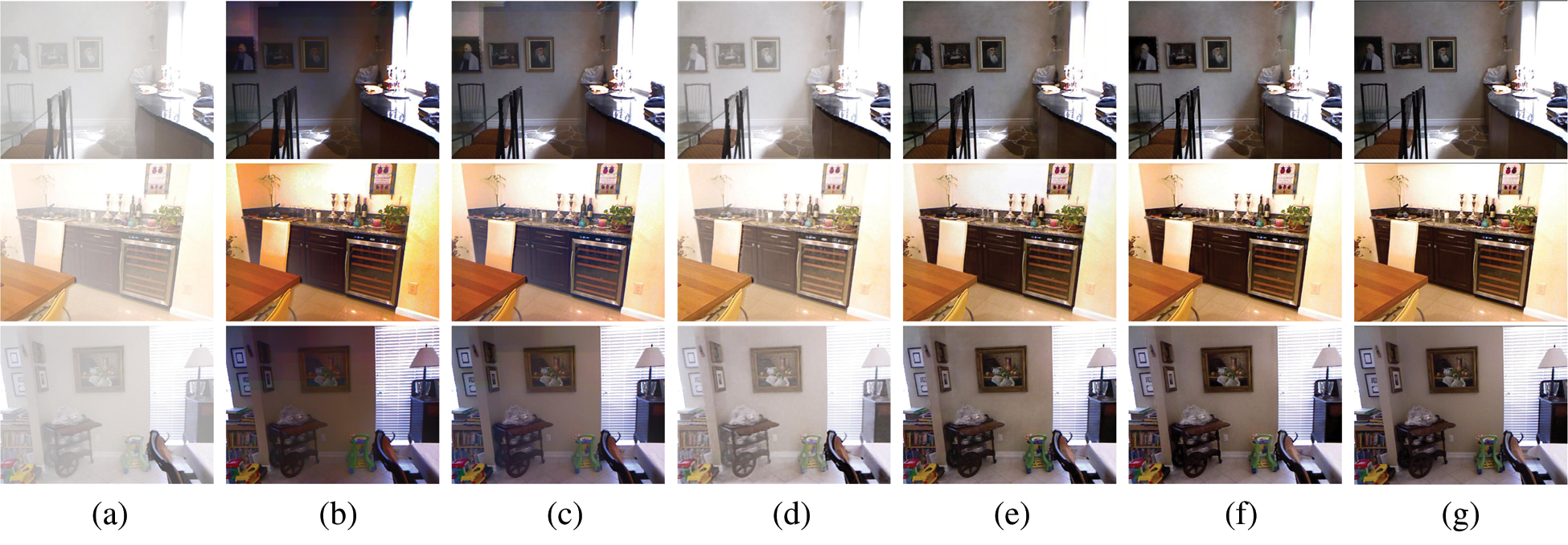
Figure 3: Indoor hazy images results. (a) Hazy, (b) DCP, (c) CAP, (d) AOD Net, (e) GCA Net, (f) Ours, (g) GT

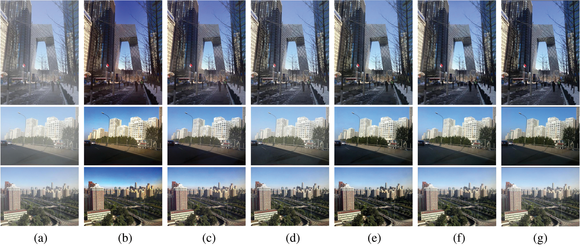
Figure 4: Outdoor hazy images results. (a) Hazy, (b) DCP, (c) CAP, (d) AOD Net, (e) GCA Net, (f) Ours, (g) GT

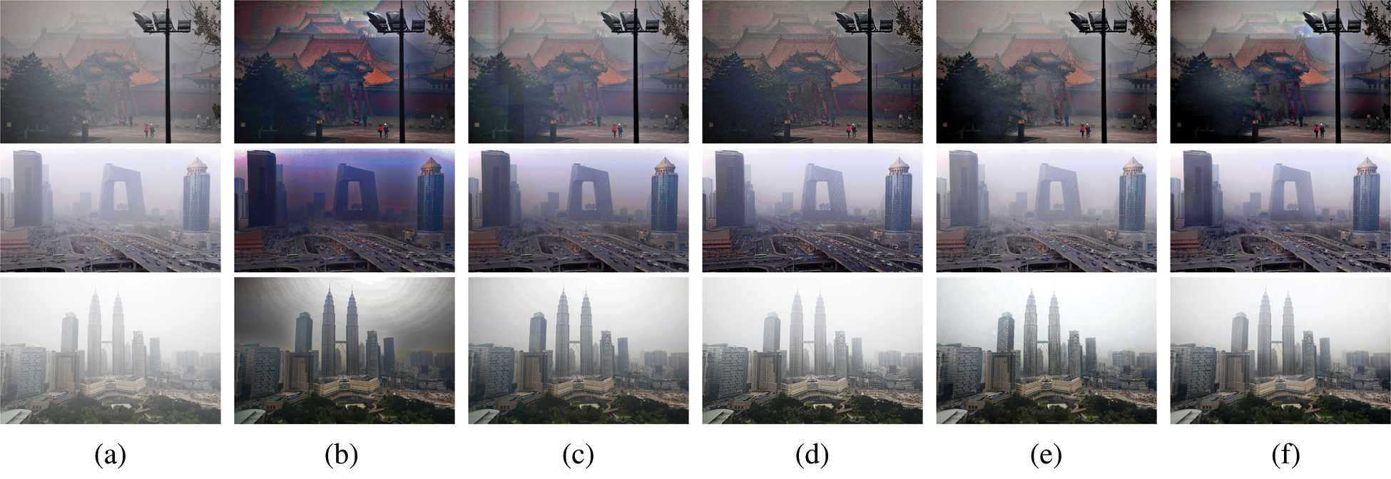
Figure 5: Real hazy images results. (a) Hazy, (b) DCP, (c) CAP, (d) AOD Net, (e) GCA Net, (f) Ours

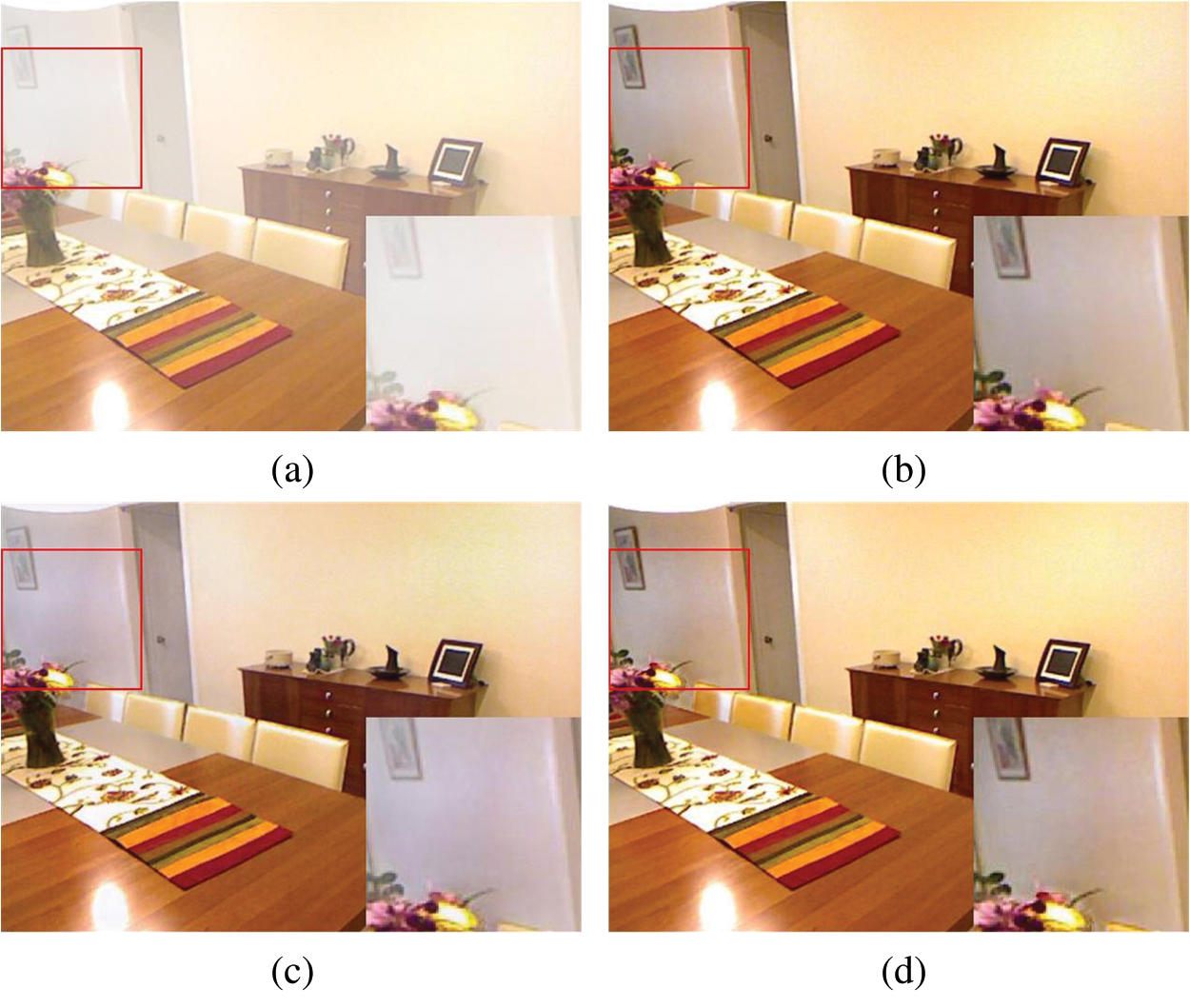
Figure 6: An example of image dehazing. (a) Hazy, (b) GT, (c) GCA Net, (d) Ours

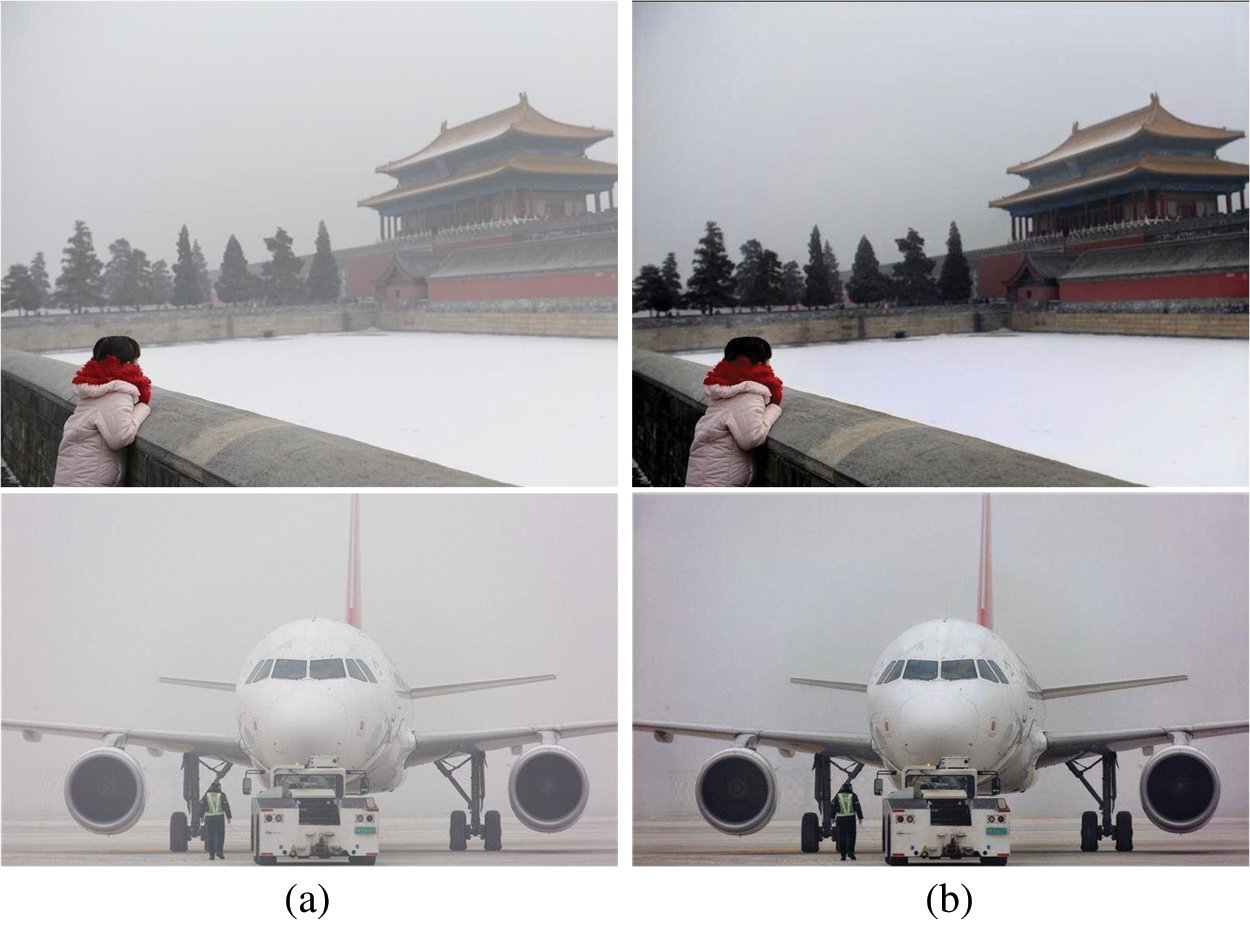
Figure 7: White scenery image dehazing results. (a) Hazy, (b) Ours

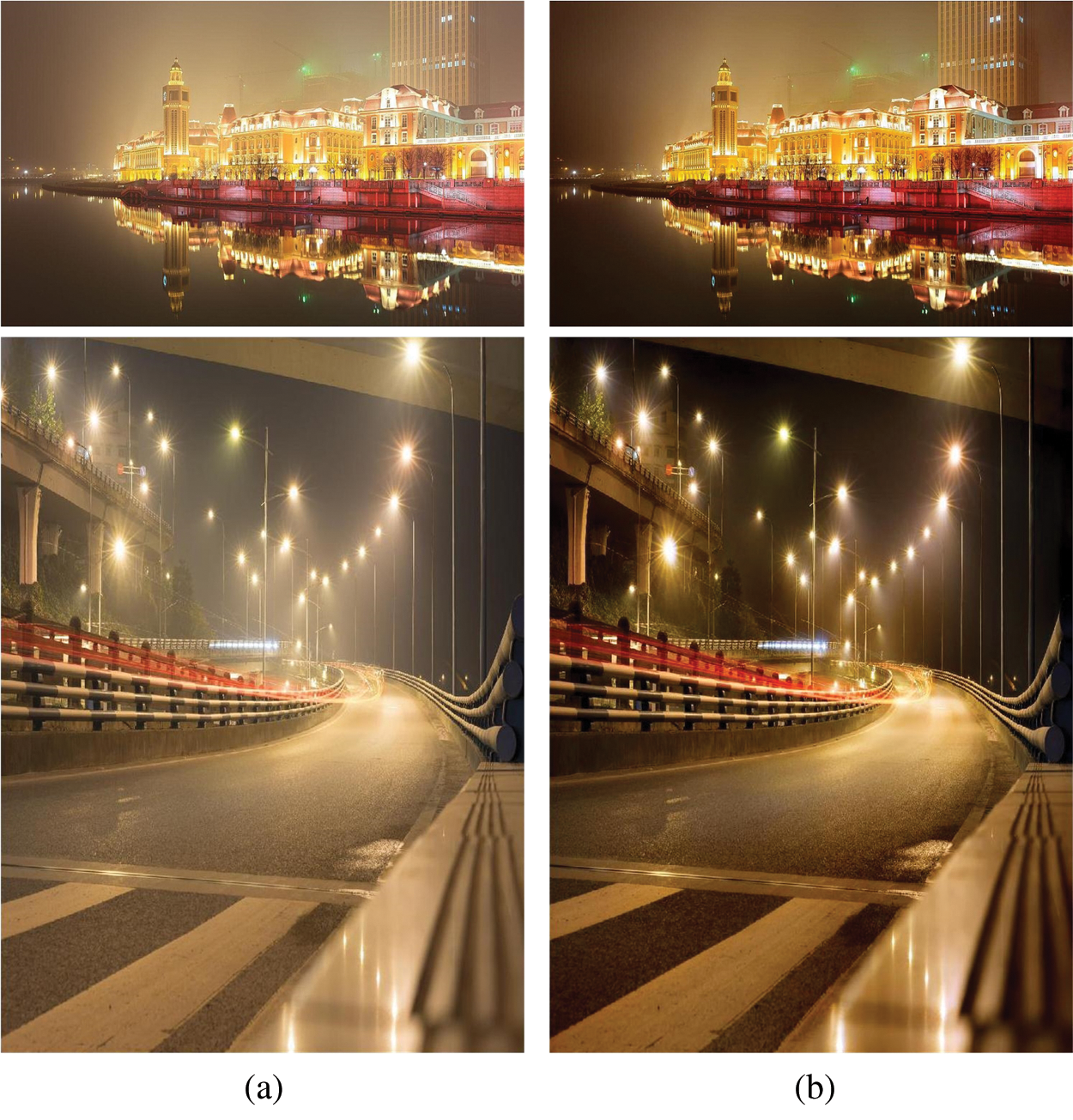
Figure 8: Examples for complex light source at night. (a) Hazy, (b) Ours

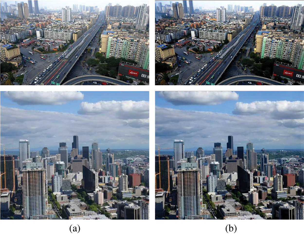
Figure 9: Examples on impacts over haze-free images, (a) Hazy, (b) Ours

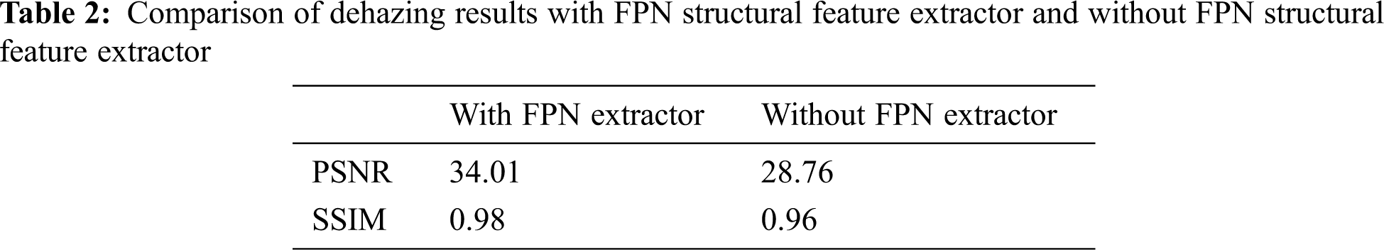
4.4 Effectiveness of FPN Structure

To verify the effectiveness of the FPN structure in dehaze, we conducted another set of comparative experiments. We directly use EfficientNet-B0 to perform feature extraction on the haze image and obtain k(x) through decoding and fusion through the decoding layer. Finally, use the dehazing model in Eq. (3) to dehaze and get a clear image. The experimental results are shown in Tab. 2. FPD-Net using the FPN structure for feature extraction has a better effect than the network directly using EfficientNet-B0 for feature extraction. Therefore, we can prove that the feature extractor of the FPN structure can more effectively extract the features of the hazy image, thereby obtaining better dehazing results.

4.5 Comparison of Running Time

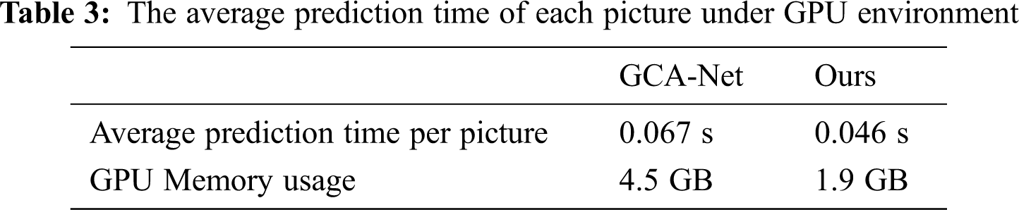
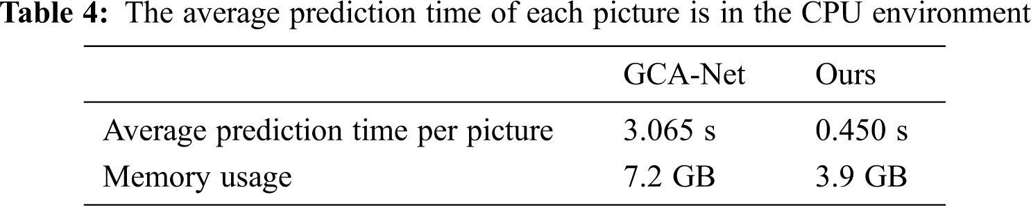
We selected 500 images from the Google RESIDE test set for testing. All dehazing methods were run on the same computer, and the average dehazing time for each image was calculated. The CPU of our experimental computer is AMD Ryzen 5 1600, the graphics card is GTX 1080ti, the memory is 16 GB, the docker environment is used for testing, and the batch size is set to 2. The average dehaze time of each picture is shown in Tab. 3. It can be seen that the speed of FPD-Net is much better than GCA-Net. And GCA-Net needs to occupy 4.5 GB of video memory during prediction, FPD-Net only needs to occupy 1.9GB of video memory. As shown in Tab. 4, the advantages of FPD-Net are more obvious when running in a CPU environment. GCA-Net takes more than 6.8 times of FPD-Net. FPD-Net has very good performance in the dehazing effect and running speed.

5  Conclusions

In this article, we propose FPD-Net. To improve the feature extraction capability of the FPD-Net, we adopted the feature extractor of FPN structure. Experiments have proved that FPD-Net has advantages over other dehaze methods in terms of PSNR, SSIM, and subjective vision. The dehaze model proposed by AOD-Net can also better reduce the loss caused by the two unknowns of the atmospheric scattering model. Besides, FPD-Net also has a considerable advantage in speed, while maintaining efficient dehaze, it also increases speed. In the future, we will try to improve the dehaze model currently used by FPD-Net to reduce the loss to even smaller. And add FPD-Net to a haze level output module to have an accurate judgment on the haze level in the picture. At the same time, we hope to use incremental learning, compressing learning and experience learning [50] to improve the speed and accuracy of the model and increase the practical value of the model.

Funding Statement: This work is supported by the Key Research and Development Program of Hunan Province (No.2019SK2161) and the Key Research and Development Program of Hunan Province (No.2016SK2017).

Conflicts of Interest: The authors declare that they have no conflicts of interest to report regarding the present study.

References

 1.  K. He, J. Sun and X. Tang, “Single image haze removal using dark channel prior,” IEEE Transactions on Pattern Analysis and Machine Intelligence, vol. 33, no. 12, pp. 2341–2353, 2010. [Google Scholar]

 2.  Q. Zhu, J. Mai and L. Shao, “A fast single image haze removal algorithm using color attenuation prior,” IEEE Transactions on Image Processing, vol. 24, no. 11, pp. 3522–3533, 2015. [Google Scholar]

 3.  D. Berman and S. Avidan, “Non-local image dehazing,” in Proc. of the IEEE Conf. on Computer Vision and Pattern Recognition, Las Vegas, NV, USA, pp. 1674–1682, 2016. [Google Scholar]

 4.  N. Hautière, J. P. Tarel and D. Aubert, “Towards fog-free in-vehicle vision systems through contrast restoration,” in 2007 IEEE Conf. on Computer Vision and Pattern Recognition, Minneapolis, MN, USA, pp. 1–8, 2007. [Google Scholar]

 5.  G. Meng, Y. Wang, J. Duan, S. Xiang and C. Pan, “Efficient image dehazing with boundary constraint and contextual regularization,” in Proc. of the IEEE Int. Conf. on Computer Vision, Sydney, Australia, pp. 617–624, 2013. [Google Scholar]

 6.  S. C. Pei and T. Y. Lee, “Nighttime haze removal using color transfer pre-processing and dark channel prior,” in 19th IEEE Int. Conf. on Image Processing, Orland, FL, USA, pp. 957–960, 2012. [Google Scholar]

 7.  B. Li, X. Peng, Z. Wang, J. Xu and D. Feng, “Aod-net: All-in-one dehazing network,” in Proc. of the IEEE Int. Conf. on Computer Vision, Venice, Italy, pp. 4770–4778, 2017. [Google Scholar]

 8.  B. Cai, X. Xu, K. Jia, C. Qing and D. Tao, “Dehazenet: An end-to-end system for single image haze removal,” IEEE Transactions on Image Processing, vol. 25, no. 11, pp. 5187–5198, 2016. [Google Scholar]

 9.  D. Chen, M. He, Q. Fan, J. Liao and L. Zhang, “Gated context aggregation network for image dehazing and deraining,” in 2019 IEEE Winter Conf. on Applications of Computer Vision (WACVWaikoloa Village, HI, USA, pp. 1375–1383, 2019. [Google Scholar]

10. C. O. Ancuti and C. Ancuti, “Single image dehazing by multi-scale fusion,” IEEE Transactions on Image Processing, vol. 22, no. 8, pp. 3271–3282, 2013. [Google Scholar]

11. T. Treibitz and Y. Y. Schechner, “Polarization: Beneficial for visibility enhancement?,” in 2009 IEEE Conf. on Computer Vision and Pattern Recognition, Miami, FL, USA, pp. 525–532, 2009. [Google Scholar]

12. Z. Wang, A. C. Bovik, H. R. Sheikh and E. P. Simoncelli, “Image quality assessment: From error visibility to structural similarity,” IEEE Transactions on Image Processing, vol. 13, no. 4, pp. 600–612, 2004. [Google Scholar]

13. A. Krizhevsky, I. Sutskever and G. E. Hinton, “Imagenet classification with deep convolutional neural networks,” Communications of the ACM, vol. 60, no. 6, pp. 84–90, 2017. [Google Scholar]

14. R. Girshick, J. Donahue, T. Darrell and J. Malik, “Rich feature hierarchies for accurate object detection and semantic segmentation,” in Proc. of the IEEE Conf. on Computer Vision and Pattern Recognition, Columbus, OH, USA, pp. 580–587, 2014. [Google Scholar]

15. K. He, G. Gkioxari, P. Dollár and R. Girshick, “Mask R-CNN,” in Proc. of the IEEE Int. Conf. on Computer Vision, Venice, Italy, pp. 2961–2969, 2017. [Google Scholar]

16. J. Ouyang, Y. He, H. Tang and Z. Fu, “Research on denoising of Cryo-em images based on deep learning,” Journal of Information Hiding and Privacy Protection, vol. 2, no. 1, pp. 1–9, 2020. [Google Scholar]

17. V. Nair and G. E. Hinton, “Rectified linear units improve restricted Boltzmann machines,” in ICML, Haifa, Israel, 2010. [Google Scholar]

18. S. Lazebnik, C. Schmid and J. Ponce, “Beyond bags of features: Spatial pyramid matching for recognizing natural scene categories,” 2006 IEEE Computer Society Conf. on Computer Vision and Pattern Recognition (CVPR’06New York, NY, USA, vol. 2, pp. 2169–2178, 2006. [Google Scholar]

19. K. Grauman and T. Darrell, “The pyramid match kernel: Discriminative classification with sets of image features,” Tenth IEEE Int. Conf. on Computer Vision, (ICCV'05) Volume 1, Beijing, China, vol. 2, pp. 1458–1465, 2005. [Google Scholar]

20. J. Yang, K. Yu, Y. Gong and T. Huang, “Linear spatial pyramid matching using sparse coding for image classification,” in 2009 IEEE Conf. on Computer Vision and Pattern Recognition, Miami, FL, USA, pp. 1794–1801, 2009. [Google Scholar]

21. K. He, X. Zhang, S. Ren and J. Sun, “Spatial pyramid pooling in deep convolutional networks for visual recognition,” IEEE Transactions on Pattern Analysis and Machine Intelligence, vol. 37, no. 9, pp. 1904–1916, 2015. [Google Scholar]

22. H. Zhao, J. Shi, X. Qi and X. Wang, “Pyramid scene parsing network,” in Proc. of the IEEE Conf. on Computer Vision and Pattern Recognition, Honolulu, HI, USA, pp. 2881–2890, 2017. [Google Scholar]

23. T. Y. Lin, P. Dollár, R. Girshick, K. He, B. Hariharan et al., “Feature pyramid networks for object detection,” in Proc. of the IEEE Conf. on Computer Vision and Pattern Recognition, Honolulu, HI, USA, pp. 2117–2125, 2017. [Google Scholar]

24. C. Song, X. Cheng, Y. X. Gu, B. J. Chen and Z. J. Fu, “A review of object detectors in deep learning,” Journal on Artificial Intelligence, vol. 2, no. 2, pp. 59–77, 2020. [Google Scholar]

25. R. Chen, L. Pan, C. Li, Y. Zhou, A. Chen et al., “An improved deep fusion CNN for image recognition,” Computers Materials & Continua, vol. 65, no. 2, pp. 1691–1706, 2020. [Google Scholar]

26. W. Wang, X. Yuan, X. Wu, Y. Liu and S. Ghanbarzadeh, “An efficient method for image dehazing,” in 2016 IEEE Int. Conf. on Image Processing (ICIPPhoenix, AZ, USA, pp. 2241–2245, 2016. [Google Scholar]

27. E. J. McCartney, “Optics of the atmosphere: Scattering by molecules and particles,” in NYJW, New York, NY, USA, pp. 698–699, 1976. [Google Scholar]

28. S. G. Narasimhan and S. K. Nayar, “Chromatic framework for vision in bad weather,” Proc. IEEE Conf. on Computer Vision and Pattern Recognition. CVPR 2000 (Cat. No. PR00662Hilton Head, SC, USA, pp. 598–605, 2000. [Google Scholar]

29. S. G. Narasimhan and S. K. Nayar, “Vision and the atmosphere,” International Journal of Computer Vision, vol. 48, no. 3, pp. 233–254, 2002. [Google Scholar]

30. M. Tan and Q. Le, “Efficientnet: Rethinking model scaling for convolutional neural networks,” in arXiv preprint arXiv:1905.11946, 2019. [Google Scholar]

31. K. He, X. Zhang, S. Ren and J. Sun, “Deep residual learning for image recognition,” in Proc. of the IEEE Conf. on Computer Vision and Pattern Recognition, Las Vegas, NV, USA, pp. 770–778, 2016. [Google Scholar]

32. G. Huang, Z. Liu, L. V. D. Maaten and K. Q. Weinberger, “Densely connected convolutional networks,” in Proc. of the IEEE Conf. on Computer Vision and Pattern Recognition, Honolulu, HI, USA, pp. 4700–4708, 2017. [Google Scholar]

33. S. Xie, R. Girshick, P. Dollár, Z. Tu and K. He, “Aggregated residual transformations for deep neural networks,” in Proc. of the IEEE Conf. on Computer Vision and Pattern Recognition, Honolulu, HI, USA, pp. 1492–1500, 2017. [Google Scholar]

34. J. Hu, L. Shen and G. Sun, “Squeeze-and-excitation networks,” in Proc. of the IEEE Conf. on Computer Vision and Pattern Recognition, Salt Lake City, UT, USA, pp. 7132–7141, 2018. [Google Scholar]

35. M. Tan, R. Pang and Q. V. Le, “Efficientdet: Scalable and efficient object detection,” in Proc. of the IEEE/CVF Conf. on Computer Vision and Pattern Recognition, Seattle, WA, USA, pp. 10781–10790, 2020. [Google Scholar]

36. S. Liu, L. Qi, H. Qin, J. Shi and J. Jia, “Path aggregation network for instance segmentation,” in Proc. of the IEEE Conf. on Computer Vision and Pattern Recognition, Salt Lake City, UT, USA, pp. 8759–8768, 2018. [Google Scholar]

37. G. Ghiasi, T. Y. Lin and Q. V. Le, “NAS-FPN: Learning scalable feature pyramid architecture for object detection,” in Proc. of the IEEE Conf. on Computer Vision and Pattern Recognition, Long Beach, CA, USA, pp. 7036–7045, 2019. [Google Scholar]

38. R. Pascanu, T. Mikolov and Y. Bengio, “On the difficulty of training recurrent neural networks,” in Int. Conf. on Machine Learning, Atlanta, GA, USA, pp. 1310–1318, 2013. [Google Scholar]

39. H. Zhang, V. Sindagi and V. M. Patel, “Multi-scale single image dehazing using perceptual pyramid deep network,” in Proc. of the IEEE Conf. on Computer Vision and Pattern Recognition Workshops, Salt Lake City, UT, USA, pp. 902–911, 2018. [Google Scholar]

40. Q. Fan, D. Chen, L. Yuan, G. Hua, N. Yu et al., “Decouple learning for parameterized image operators,” in Proc. of the European Conf. on Computer Vision (ECCVMunich, Germany, pp. 442–458, 2018. [Google Scholar]

41. Q. Fan, J. Yang, G. Hua, B. Chen and D. Wipf, “A generic deep architecture for single image reflection removal and image smoothing,” in Proc. of the IEEE Int. Conf. on Computer Vision, Venice, Italy, pp. 3238–3247, 2017. [Google Scholar]

42. Y. Li, R. T. Tan, X. Guo, J. Lu and M. S. Brown, “Rain streak removal using layer priors,” in Proc. of the IEEE Conf. on Computer Vision and Pattern Recognition, Las Vegas, NV, USA, pp. 2736–2744, 2016. [Google Scholar]

43. H. Li, C. Pan, Z. Chen, A. Wulamu and A. Yang, “Ore image segmentation method based on u-net and watershed,” Computers Materials & Continua, vol. 65, no. 1, pp. 563–578, 2020. [Google Scholar]

44. R. Li, J. Pan, Z. Li and J. Tang, “Single image dehazing via conditional generative adversarial network,” in Proc. of the IEEE Conf. on Computer Vision and Pattern Recognition, Salt Lake City, UT, USA, pp. 8202–8211, 2018. [Google Scholar]

45. H. Zhang and V. M. Patel, “Densely connected pyramid dehazing network,” in Proc. of the IEEE Conf. on Computer Vision and Pattern Recognition, pp. 3194–3203, 2018. [Google Scholar]

46. A. Paszke, S. Gross, S. Chintala, G. Chanan, E. Yang et al., “Automatic differentiation in pytorch,” 2017. [Google Scholar]

47. B. Li, W. Ren, D. Fu, D. Tao, D. Feng et al., “Reside: A benchmark for single image dehazing,” in arXiv preprint arXiv:1712.04143, 2017. [Google Scholar]

48. H. Wu, Q. Liu and X. Liu, “A review on deep learning approaches to Image classification And object segmentation,” Computers Materials & Continua, vol. 60, no. 2, pp. 575–597, 2019. [Google Scholar]

49. W. Ren, L. Ma, J. Zhang, J. Pan, X. Cao et al., “Gated fusion network for single image dehazing,” in Proc. of the IEEE Conf. on Computer Vision and Pattern Recognition, Salt Lake City, UT, USA, pp. 3253–3261, 2018. [Google Scholar]

50. F. Jiang, K. Wang, L. Dong, C. Pan, W. Xu et al., “AI driven heterogeneous MEC System with UAV assistance for dynamic environment: challenges and solutions,” IEEE Network, vol. 35, no. 1, pp. 400–408, 2021. [Google Scholar]

This work is licensed under a Creative Commons Attribution 4.0 International License, which permits unrestricted use, distribution, and reproduction in any medium, provided the original work is properly cited.