DOI:10.32604/csse.2022.020175
| Computer Systems Science & Engineering DOI:10.32604/csse.2022.020175 | |
| Article |
Solvability of the Nonlocal Inverse Parabolic Problem and Numerical Results
1Department of Mathematics, College of Science, Jazan University, Jazan, Saudi Arabia
2Department of Mathematics and Informatics, Larbi Ben M’hidi University, Oum El Bouaghi, Algeria
*Corresponding Author: M. J. Huntul. Email: mhantool@jazanu.edu.sa
Received: 11 May 2021; Accepted: 12 June 2021
Abstract: In this paper, we consider the unique solvability of the inverse problem of determining the right-hand side of a parabolic equation whose leading coefficient depends on time variable under nonlocal integral overdetermination condition. We obtain sufficient conditions for the unique solvability of the inverse problem. The existence and uniqueness of the solution of the inverse parabolic problem upon the data are established using the fixed point theorem. This inverse problem appears extensively in the modelling of various phenomena in engineering and physics. For example, seismology, medicine, fusion welding, continuous casting, metallurgy, aircraft, oil and gas production during drilling and operation of wells. In addition, the numerical solution of the inverse problem is studied by using the Crank-Nicolson finite difference method together with the Tikhonov regularization to find a stable and accurate approximate solution of finite differences. The resulting nonlinear system of parabolic equation is solved computationally using the MATLAB subroutine lsqnonlin. Both analytical and numerically simulated noisy input data are inverted. The root mean square error values for various noise levels for both continuous and discontinuous time-dependent heat source term are compared. Numerical results presented for two examples show the efficiency of the computational method and the accuracy and stability of the numerical solution even in the presence of noise in the input data. Furthermore, the choice of the regularization parameter is also discussed based on the trial and error technique.
Keywords: Inverse problem; nonlocal integral condition; fixed point theorem; Tikhonov regularization; nonlinear optimization
Inverse boundary value problems arise in various areas of human activity such as mineral exploration, seismology, medicine, biology, quality control in industry, etc., which makes them an active field of contemporary mathematics and physics. Inverse problems for parabolic equations satisfying nonlocal integral overdetermination conditions were first studied in [1–8] for equations with coefficients independent of time and boundary conditions of the first and third kind. These papers contain the proof of theorems on the equivalence of the original inverse problem to an operator equation of the second kind with a totally continuous operator. Moreover, Cannon et al. [9,10] investigated the inverse problem of identifying the perfusion, and source control coefficients and the temperature, respectively. Kamynin [11] proved the unique solvability of the inverse problem of finding the right-hand side of a parabolic equation with the leading coefficient depending on time and space variables under a final overdetermination condition while Kamynin [12] discussed the existence of the solution to the initial-boundary problem for the parabolic equation.
In this paper, we study the existence and uniqueness of the inverse problem of determining a pair of functions {u(x, t), f(t)} satisfying the parabolic equation
where Ω is a bounded domain in ℝn with smooth boundary ∂Ω. The functions g(x, t), φ(x), v(x), θ(t) are known and β is a given positive constant.
Nonclonal integral specifications condition of the form Eq. (4) arises from many important applications in heat transfer, mass/energy, thermoelasticity, control theory, life science, etc. [13–17]. For instance, for heat propagation in a thin rod in which the law of variation θ(t) of the total quantit of heat in the rod is given in [18]. In addition, the inverse problem of determining the time-dependent coefficient in a one and two-dimensional parabolic equation from nonlocal integral over-specification condition has been investigated widely by many researchers in the past, see [19–23] to mention only a few.
In the present paper, the existence and uniqueness of the inverse problem Eqs. (1)–(4) are established using the fixed point theorem. We have also investigated the numerical solution of the inverse problem. Moreover, the novelty consists in the development of a convergent numerical optimization method for solving this nonlinear inverse coefficient problem for the parabolic equation. Numerically, the implementation is realised using the MATLAB subroutine lsqnonlin.
The rest of the paper is organized as follows. Section 2 illustrates the preliminaries. The unique solvability of the inverse problem is given in Section 3. The numerical solution of the direct (forward) problem based on the finite difference method with a Crank-Nicolson scheme is given in Section 4. In Section 5, the numerical solution to solve the inverse problem based on a minimization of the Tikhonov objective functional is given. Numerical results are presented and discussed in Section 6. Finally, conclusions are stated in Section 7.
We begin with certain notations and definition as:
Definition 2. We denote the space L2(Ω) by
3 Unique Solvability of the Inverse Problem
Definition 3. By a generalized solution of problem Eqs. (1)–(4), we mean a pair of functions {u(x, t), f(t)},
We seek a solution of the original inverse problem as
where y(x, t) is the solution (in QT) of the original problem
where
where
Remark. As {u, f} = {z, f} + {y, 0}, where y is the solution of the direct problem Eqs. (7)–(9). It is clear that the solution y exists and is unique by the previous section. So instead of studying the main inverse problem Eqs. (1)–(4), it is enough to study the inverse problem Eqs. (10)–(14).
Theorem 1. Suppose that the input data of the inverse problem Eqs. (10)–(14) satisfies the conditions (A1) and (A2). Then we have the equivalent between the following assumptions:
(i)if the inverse problem Eqs. (10)–(14) has a unique solution, then so is Eq. (17), and
(ii)if the Eq. (17) possesses a solution and verify the compatibility conditionE(0) = 0, then there exists a solution of the inverse problem Eqs. (10)–(14).
Proof. (i) Suppose that the problem Eqs. (10)–(14) is solvable. Let {z, f} be the solution of the inverse problem Eqs. (10)–(14). Now, multiplying equation Eq. (10) by the function v and integrating over Ω, we obtain
(ii) Now, we suppose that the Eq. (17) has a solution in the space L2(0, T), and so be f. If inserting the function f in Eq. (10), then resulting relations Eqs. (10)–(13) can be considered as a direct problem with a unique solution
It remains to show that the function z verifies the condition Eq. (13). Form the using of the Eq. (19), it yields that
By subtracting the Eq. (20) from the Eq. (21), we obtain
Integrating the previous differential equation and taking into account the compatibility condition E(0) = 0 into account, we conclude that z satisfies Eq. (13), and finally, we find that the pair of functions {z, f} is a solution of the original inverse problem Eqs. (10)–(14). This completes the proof of Theorem 1.
Lemma 1. Suppose that the conditions (A1) and (A2) be fulfilled. Then, for which A is a contracting operator in L2(0, T).
Proof. Definitely, Eq. (16) gives the estimate
where
where
Theorem 2. Let the conditions (A1), (A2), and the compatibility condition E(0) = 0 be satisfied. Then the assertions:
(i)a solution {z, f} of the inverse problem Eqs. (10)–(14) exists and is unique, and
(ii)with any initial iteration f0 ∈ L2(0, T), the successive approximations
Proof. (ii) We use the following operator
where the operator A and the function
This shows that, Eqs. (33) and (17) have a unique solution f in L2(0, T). Hence, according to the Theorem 1, this validates the existence of solution to the inverse problem Eqs. (10)–(14). Now, it remains to show the uniqueness of this solution. Using the proof by the contrary, for this we a ssume that there are two distinct solutions {z1, f1} and {z2, f2} of the main inverse problem. Firstly, we start by the case f1 ≠ f2 almost everywhere on (0, T). Since, if f1 = f2, then the theorem of the uniqueness or the direct problem of Eqs. (7)–(9) gives z1 = z2 almost everywhere in QT. Thus, as both pairs verify Eq. (20), we obtain that the two f1 and f2 functions are different solutions of Eq. (34), which contradicts the uniqueness of the solution of Eq. (34). This completes the proof of Theorem 2. ◼
Corollary 1. Let the assumptions of Theorem 2 be fulfilled, and then the solution f depends continuously with respect to the data W of the Eq. (17).
Proof. Suppose W and V are two sets of data satisfying the assumptions of Theorem 2. Let f and g be two solutions of Eq. (17) corresponding to W and V, respectively. According to Eq. (17), we have
This completes the proof of Corollary 1. ◼
4 Numerical Solution of the Direct Problem
The numerical scheme of the one-dimensional (n = 1) initial-boundary value problem Eqs. (1)–(3) can be established using the Crank-Nicolson FDM, see e.g., [24], which is unconditionally stable and second-order accurate in space x and time t, when f(t) and g(x, t) are known and the solution u(x, t) is to be determined together with the quantity of interest θ(t). Set the domain Ω = (0, 1), and QT = (0, 1) × (0, T). For numerical discretization, a rectangular network is constructed by subdividing the domain QT into M and N subintervals of equal lengths Δx and Δt, where Δx = 1/M and Δt = T/N, respectively. At the node (i, j) we denote u(xi, tj) = ui,j, where xi = iΔx, tj = jΔt, f(tj) = fj, and g(xi, tj) = gi,j for
where
5 Numerical Solution of the Inverse Problem
Our aim is to obtain stable and accurate identification for the heat source f(t) along with the temperature u(x, t) satisfing Eqs. (1)–(4). The inverse problem is formulated as minimizing the regularized nonlinear Tikhonov function
where u solves numerically using the Crank-Nicolson FDM [24] the forward problem Eqs. (1)–(3) for given f(t), and λ ≥ 0 is regularization parameter which is initiated for stabilizing the numerical results. In discrete form, Eq (43) becomes
The unregularized case, i.e., λ = 0, yields the ordinary nonlinear least-squares method which is usually producing unstable solutions when noisy data are inverted. The minimization of the objective function (44) is carried out utilizing the MATLAB subroutine lsqnonlin [25]. This iterative routine attempts to solve a nonlinear least-squares minimization problem, starting from an initial guess, subject to constraints, and this generally is referred to as a constrained nonlinear optimization. We use the Trust-Region-Reflective (TRR) optimization algorithm from lsqnonlin based on the interior-reflective Newton method, and some details about how this is implemented for the minimization of a least-squares functional Eq. (44) has recently been given in [26].
The noisy data is numerically simulated as
where εj are random variables generated from a Gaussian normal distribution with mean zero and standard deviation σ given by
where p denotes the percentage of noise.
6 Numerical Results and Discussion
In this section, the numerical methods for reconstructing the time-dependent source term f(t) alonge with the temperature u(x, t) are illustrated, and two numerical experiments based on the FDM with the Crank-Nicolson established in the previous section are shown. We measure the accuracy by rmse [27–29]:
We take T = 1, for simplicity. The lower and upper bounds for the heat source f(t) are taken as − 102 and 102, respectively.
First, we consider the inverse problem Eqs. (1)–(4) with a smooth unknown heat source term f(t), with the following input data:
where Ω is a bounded domain in [0, 1]. The exact solution to this inverse problem is given by
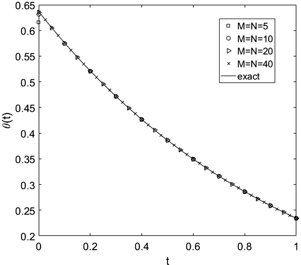
Figure 1: The exact Eq. (49) and numerical solutions for θ(t), with various mesh sizes M = N ∈ {5, 10, 20, 40}, for direct problem
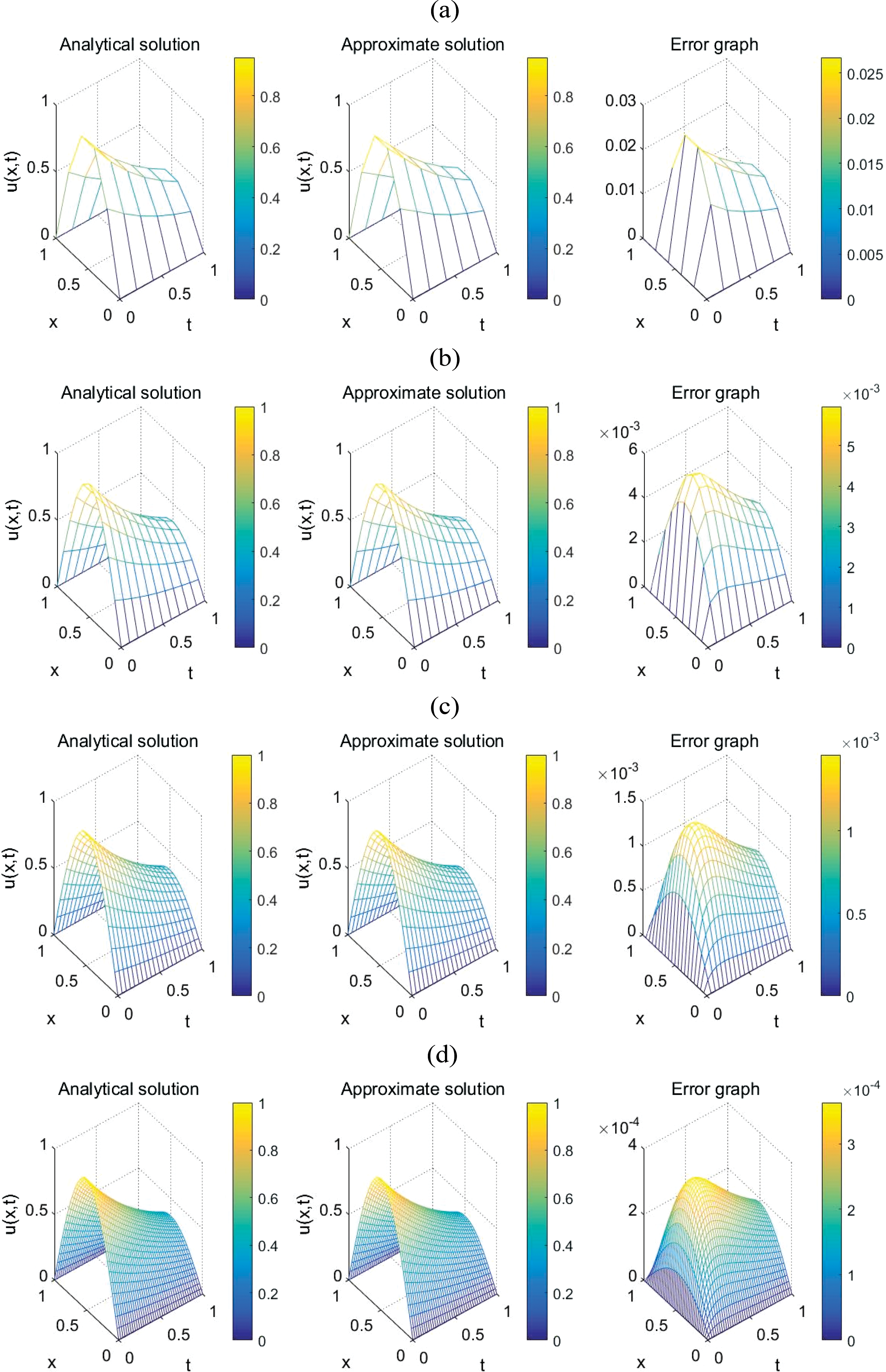
Figure 2: The exact Eq. (50) and numerical temperature u(x, t), for direct problem with vaiuous grid sizes for: (a) M = N = 5, (b) M = N = 10, (c) M = N = 20 and (d) M = N = 40. The absolute errors between them are also included
Next, let us fix Δx = Δt = 0.025 and start the investigation of determining the coefficient f(t), where there is no noise, i.e., p = 0, in the measured data θ(t), as in Eq. (46). The objective function J, as a function of the number of iterations, is depicted in Fig. 3a. From this figure it can be seen that a fast convergence is achieved in 4 iterations to reach a very low value of O(10−30). Fig. 3b illustrates the numerical solutions for the heat source f(t). From Fig. 3b it can be seen that there is an excellent agreement between the exact Eq. (51) and numerical solutions with rmse(f) =5.4E − 5.
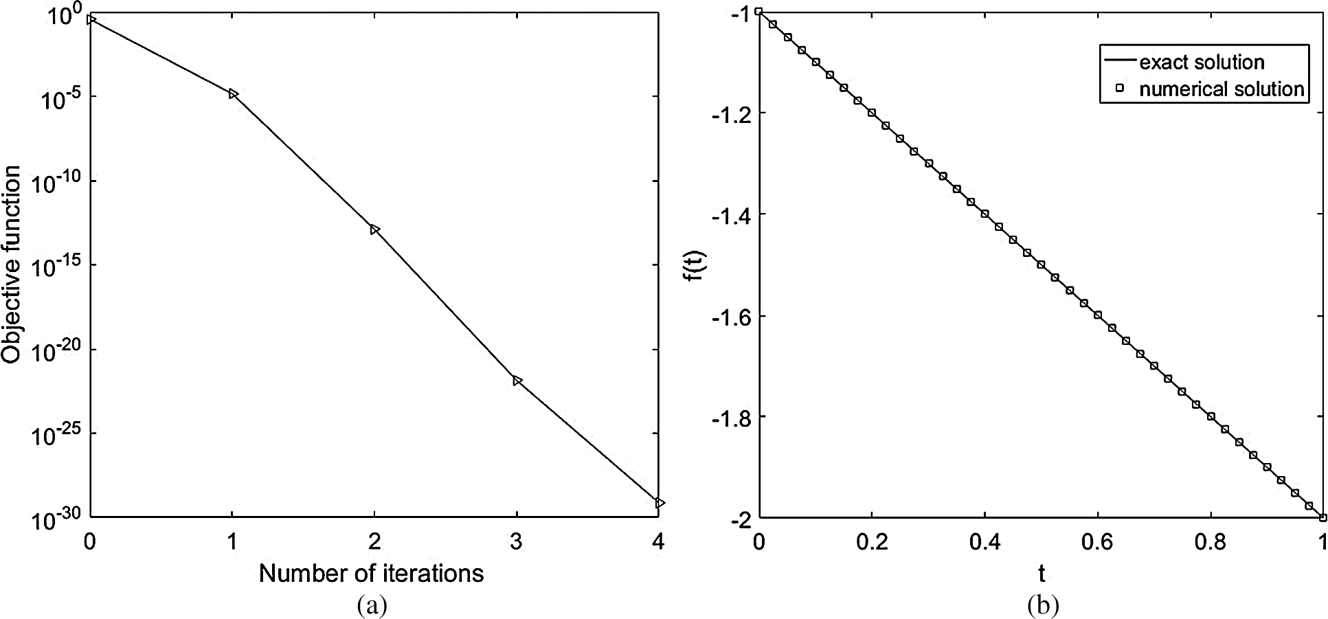
Figure 3: (a) The objective function J Eq. (44), as a function of the number of iterations, and (b) the exact Eq. (51) and numerical solutions for the heat source f(t), with no noise and no regularization, for Example 1
Now, the stability of the approximate solution is examined with respect to the perturbed (noisy measured) data Eq. (45). We include various noise levels p ∈ {1%, 3%} to the input data Eq. (48). Figs. 4 and 5 show the reconstruction of the estimated f(t). The heat source f(t) is depicted in Figs. 4a and 5a, where the unstable and inaccurate results are obtained, if no regularization, i.e., λ = 0, is imposed with rmse(f) = 0.7134 for p = 1%, and ..)=2.1384 for
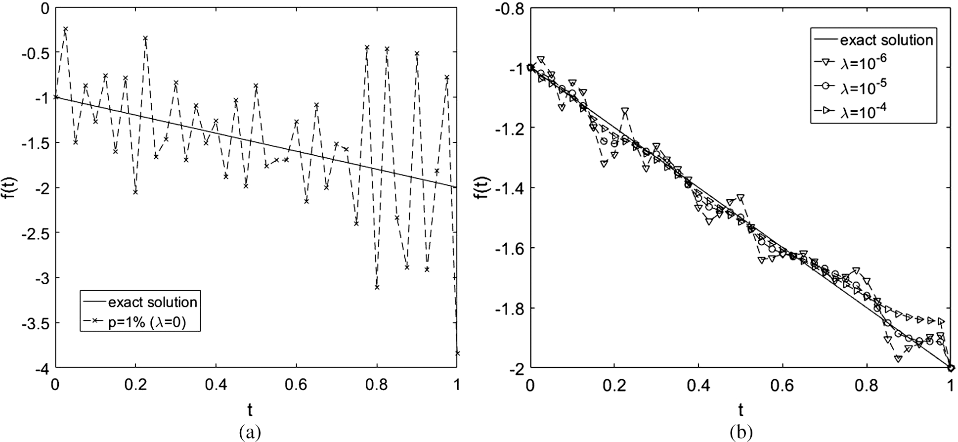
Figure 4: The exact Eq. (51) and numerical solutions for the heat source f(t), with p = 1% noise and with and without regularization, for Example 1
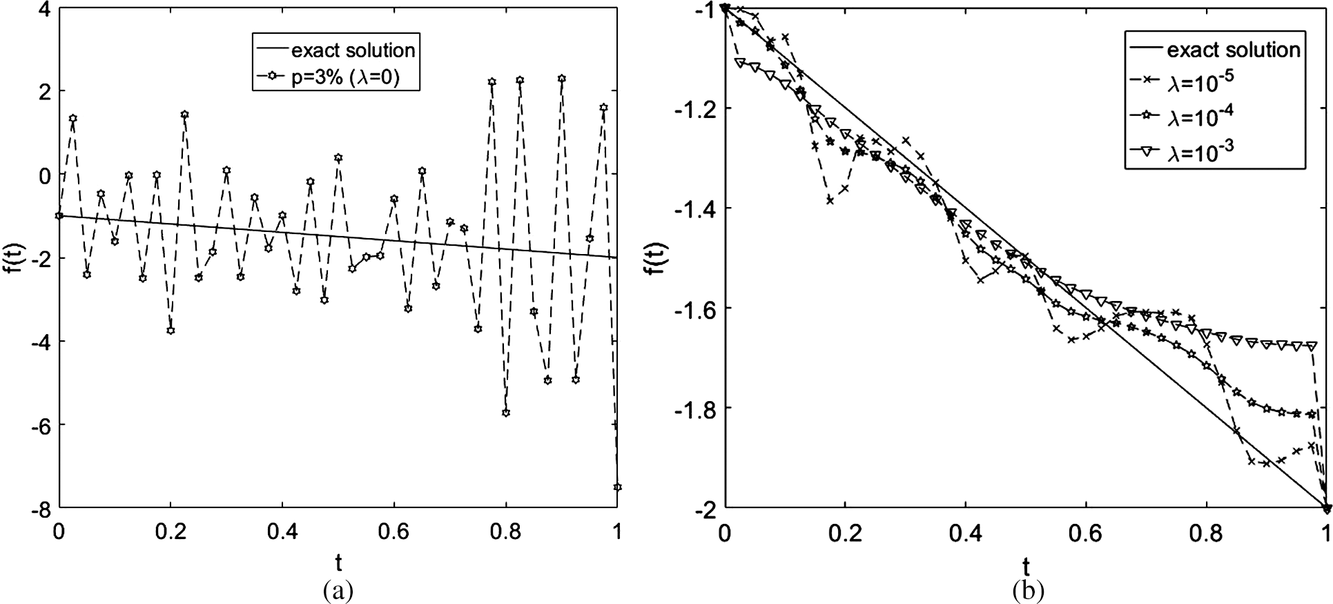
Figure 5: The exact Eq. (51) and numerical solutions for the heat source f(t), with p = 3% noise and with and without regularization, for Example 1
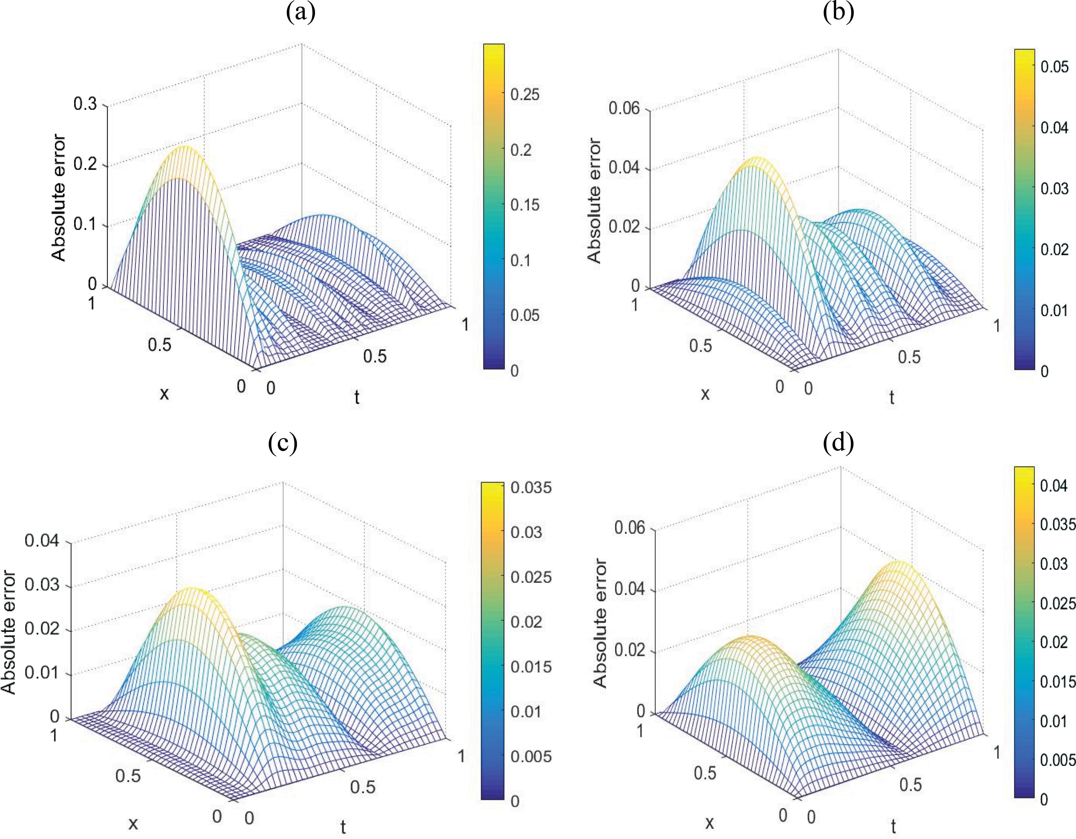
Figure 6: The absolute errors between the exact Eq. (50) and numerical temperature u(x, t), for Example 1 with p = 3% noise: (a) λ = 0, (b) λ = 10−5, (c) λ = 10−4, and (d) λ = 10−3
In the previous example we have inverted a smooth coefficient given by Eq. (51). In this example, we consider the recovery of a non-smooth (discontinuous) function for the heat source f(t) for the inverse problem given by Eqs. (1)–(4) with the following input data:
We investigate the inverse problem as we did in Example 1. We take and determining the unknown force coefficient f(t) along with the temperature u(x, t) for exact measured input data Eq. (45), i.e., p = 0, in Eq. (46). Although not illustrated, it is reported that a rapid monotonic decreasing convergence of the objective function Eq. (44) to a very small minimum value of O(10−30) is achieved in about 6 iterations. The exact Eq. (53) and numerical results for f(t) are depicted in Fig. 7. From this figure, it can be seen that the recovered coefficient is in very good agreement with their corresponding analytical solutions with rmse(f)= 6.2E − 4.
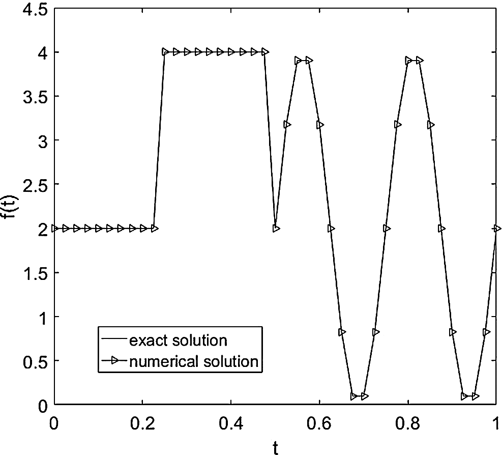
Figure 7: The exact Eq. (53) and numerical solutions for the heat source f(t), with no noise and no regularization, for Example 2
In order to investigate the stability of the solution we add p ∈ {0.5%, 1%} noise to the input data Eq. (4), as in Eq. (46). We have also investigated higher amounts of noise p in Eq. (46), but the results obtained were less accurate and therefore, they are not presented. The corresponding numerical results for the unknown coefficient are presented in Figs. 8 and 9. From Figs. 8a and 9a it can be seen that unstable results are obtained for f(t) (compare with the results for exact data in Fig. 7) with rmse(f) = 0.5625 and 1.1192, respectively. This is expected since the problem under investigation is ill-posed and very sensitive to noise. Consequently, regularization should be applied to restore the stability of the solution in the component f(t). We selected the regularization parameter λ ∈ {10−8, 10−7} for p = 0.5% noise (see Fig. 8b), and λ ∈ {10−7, 10−6} for p = 1% noise (see Fig. 9b), which give stable and reasonablly accurate solutions for the heat source coefficient f(t), obtaining rmse(f) ∈ {0.2070, 0.1899} and rmse(f) ∈ {0.2203, 0.3648}. One of the main difficulties when we solve inverse and ill-posed problems is how to choose an appropriate regularization parameter λ which must compromise between accuracy and stability. Nevertheless, one can use techniques such as the L-curve method [30] or, Morozov’s discrepancy principle [31] to find such a parameter, but in our work we have used trial and error. As mentioned in [32], the regularization parameter λ is selected based on experience by first choosing a small value and gradually increasing it until any numerical oscillations in the unknown coefficient are removed. Overall, the numerical results obtained by using the methods established in this paper, i.e., the FDM with a Crank-Nicolson combined with the minimization of the nonlinear Tikhonov regularization functional using the MATLAB optimization toolbox routine lsqnonlin illustrate that accurate and stable solutions can be obtained for reconstructing the time-dependent coefficient f(t) in parabolic PDE.
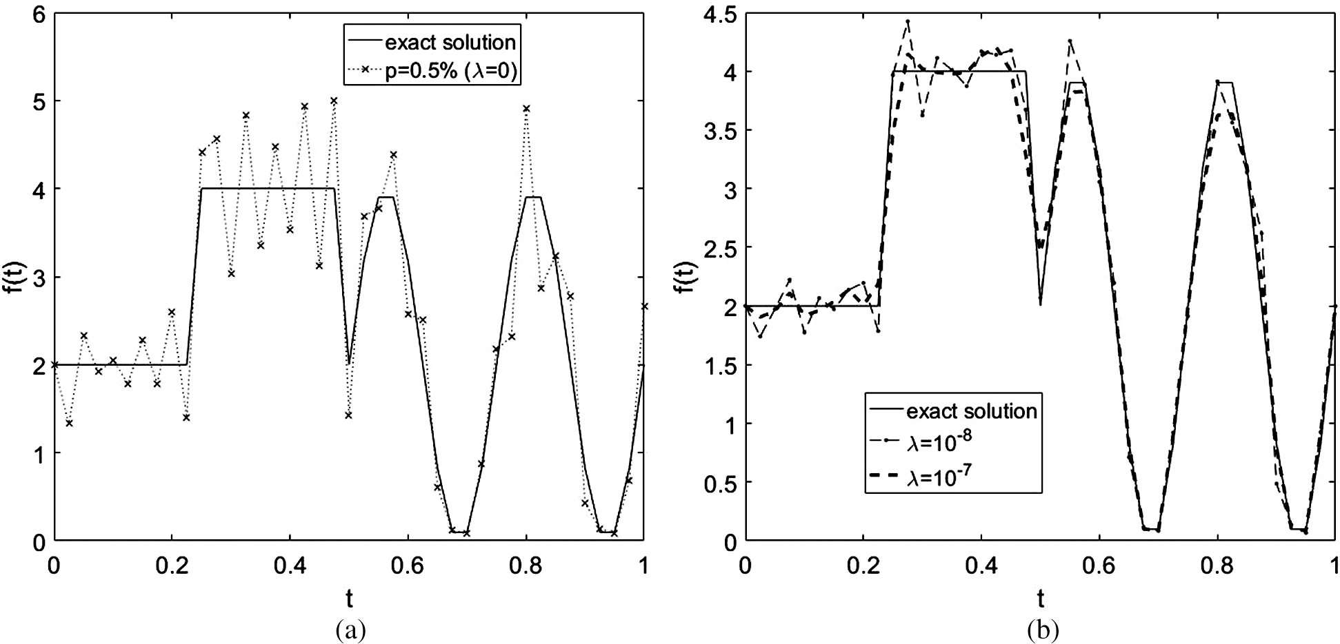
Figure 8: The exact Eq. (53) and numerical solutions for the heat source f(t), with p = 0.5% noise and with and without regularization, for Example 2
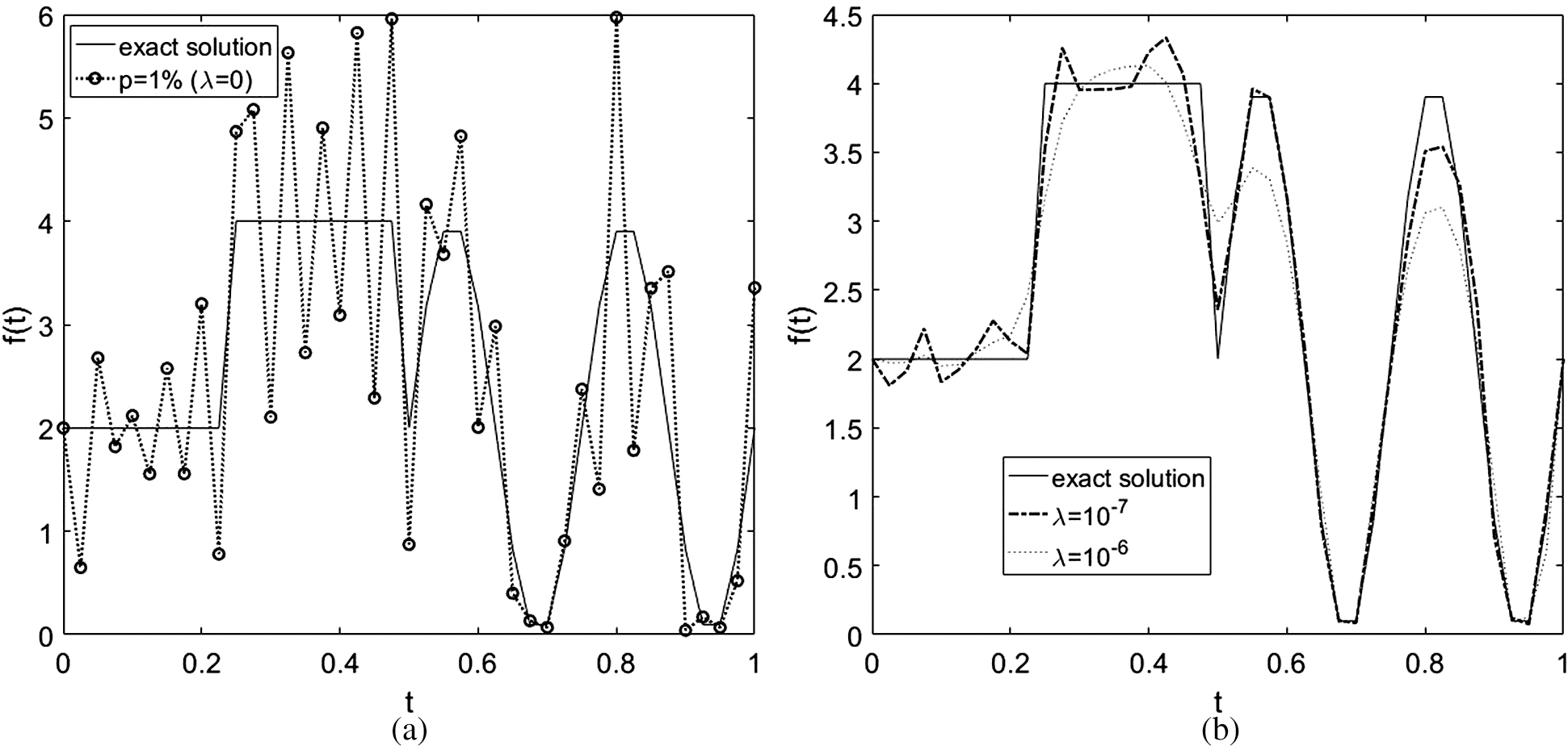
Figure 9: The exact Eq. (53) and numerical solutions for the heat source f(t), with p = 1% noise and with and without regularization, for Example 2.
In this paper, the inverse problem involving the determination of the time-dependent component and the temperature in the parabolic heat Eq. (1) from the nonlocal integral over-specification condition (4) has been investigated theoretically as well as numerically. Sufficient conditions which ensure the unique solvability of a local solution are provided and proved. The direct solver based on the Crank-Nicolson FDM has been employed. The inverse problem solution based on a nonlinear least-squares minimization problem has been solved using the MATLAB optimisation toolbox routine lsqnonlin. The Tikhonov regularization has been applied in order to obtain stable and accurate solutions since the inverse problem is ill-posed (small errors in the nonlocal integral input data cause large errors in the output force) and sensitive to noise. Two numerical examples for one-dimensional inverse problem have been illustrated for continuous and discontinuous heat source coefficient. Numerical results presented and discussed for both exact and noisy data show that accurate and stable solutions have been obtained. Finally, the generalization of the proposed numerical method for determining the time-dependent coefficient in a two-dimensional parabolic equation is an interesting topic for future research.
Acknowledgement: The authors are indebted to the anonymous referees for their valuable comments and suggestions that helped improve the paper.
Funding Statement: The authors received no specific funding for this study.
Conflicts of Interest: No potential conflict of interest was reported by the authors.
1. V. L. Kamynin, “On the solvability of the inverse problem for determining the right-hand side of a degenerate parabolic equation with integral observation,” Matematicheskie Zametki, vol. 98, pp. 710–724, 2015. [Google Scholar]
2. M. Ivanchov, “I nverse Problems for Equations of Parabolic Type,” VNTL Publishers, Lviv, Ukraine, 2003. [Google Scholar]
3. F. Kanca and M. Ismailov, “Inverse problem of finding the time-dependent coefficient of heat equation from integral overdetermination condition data,” Inverse Problems in Science and Engineering, vol. 20, pp. 463–476, 2012. [Google Scholar]
4. A. B. Kostin, “Inverse problem for the heat equation with integral overdetermination,” Moscow Institute of Engineering Physics, Moscow, vol. 1991, pp. 45–49, 1991. [Google Scholar]
5. A. I. Prilepko and A. B. Kostin, “On inverse problems for parabolic equations with final and integral overdetermination,” Matematicheskii Sbornik, vol. 183, pp. 49–68, 1992. [Google Scholar]
6. A. I. Prilepko and A. B. Kostin, “On inverse problems of determining a coefficient in a parabolic equation, II,” Sibirskii Matematicheskii Zhurnal, vol. 34, pp. 147–162, 1993. [Google Scholar]
7. A. I. Prilepko and I. V. Tikhonov, “Reconstruction of an inhomogeneous summand in an abstract evolution equation,” Izv. Ross. Akad. Nauk Ser. Mat, vol. 58, pp. 167–188, 1994. [Google Scholar]
8. O. Taki-Eddine and B. Abdelfatah, “On determining the coefficient in a parabolic equation with nonlocal boundary and integral condition,” Electronic Journal of Mathematical Analysis and Applications, vol. 6, pp. 94–102, 2018. [Google Scholar]
9. J. R. Cannon and S. Wang, “Determination of a control parameter in a parabolic partial differential equation,” Journal of the Australian Mathematical Society Series B-Applied Mathematics, vol. 33, pp. 149–163, 1991. [Google Scholar]
10. J. R. Cannon and S. Wang, “Determination of source parameter in a parabolic equations,” Meccanica, vol. 27, pp. 85–94, 1992. [Google Scholar]
11. V. L. Kamynin, “On the unique solvability of an inverse problem for parabolic equations under a final overdetermination condition,” Mathematical Notes, vol. 73, pp. 202–211, 2003. [Google Scholar]
12. V. L. Kamynin, “On the inverse problem of determining the leading coefficient in a parabolic equation,” Matematicheskie Zametki, vol. 84, pp. 48–58, 2008. [Google Scholar]
13. J. R. Cannon and J. van der Hoek, “The one phase stefan problem subject to the specification of energy,” Journal of Mathematical Analysis and Applications, vol. 86, pp. 281–291, 1982. [Google Scholar]
14. J. R. Cannon and J. van der Hoek, “Diffusion subject to the specification of mass,” Journal of Mathematical Analysis and Applications, vol. 115, pp. 517–529, 1986. [Google Scholar]
15. A. Fatullayev, N. Gasilov and I. Yusubov, “Simultaneous determination of unknown coefficients in a parabolic equation,” Applicable Analysis, vol. 86, pp. 1167–1177, 2008. [Google Scholar]
16. M. Ivanchov and N. Pabyrivska, “Simultaneous determination of two coefficients of a parabolic equation in the case of nonlocal and integral conditions,” Ukrainian Mathematical Journal, vol. 53, pp. 674–684, 2001. [Google Scholar]
17. M. Ismailov and F. Kanca, “An inverse coefficient problem for a parabolic equation in the case of nonlocal boundary and overdetermination conditions,” Mathematical Methods in the Applied Sciences, vol. 34, pp. 692–702, 2011. [Google Scholar]
18. N. I. Ionkin, “Solution of a boundary-value problem in heat conduction with a non-classical boundary condition,” Differential Equations, vol. 13, pp. 204–211, 1977. [Google Scholar]
19. M. J. Huntul and D. Lesnic, “An inverse problem of finding the time-dependent thermal conductivity from boundary data,” International Communications in Heat and Mass Transfer, vol. 85, pp. 147–154, 2017. [Google Scholar]
20. M. J. Huntul, D. Lesnic and M. S. Hussein “Reconstruction of time-dependent coefficients from heat moments,” Applied Mathematics and Computation, vol. 301, pp. 233–253, 2017. [Google Scholar]
21. M. J. Huntul, D. Lesnic and B. T. Johansson “Determination of an additive time- and space-dependent coefficient in the heat equation,” International Journal of Numerical Methods for Heat and Fluid Flow, vol. 28, no. 6, pp. 1352–1373, 2018. [Google Scholar]
22. M. J. Huntul, “Reconstructing the time-dependent thermal coefficient in 2D free boundary problems,” CMC-Computers, Materials & Continua, vol. 67, no. 3, pp. 3681–3699, 2021. [Google Scholar]
23. M. J. Huntul, “Finding the time-dependent term in 2D heat equation from nonlocal integral conditions,” Computer Systems Science and Engineering, accepted, 2021. [Google Scholar]
24. G. D. Smith, “N umerical Solution of Partial Differential Equations: Finite Difference Methods,” Clarendon Press, Oxford, Third edition, 1985. [Google Scholar]
25. Mathworks, “Documentation optimization toolbox-least squares (Model fitting) algorithms,” 2019. [Online]. Available: https://www.mathworks.com. [Google Scholar]
26. K. Ito and J. C. Liu, “Recovery of inclusions in 2D and 3D domains for poisson’s equation,” Inverse Problems, vol. 29, pp. 20pages, 2013. [Google Scholar]
27. N. Khalid, M. Abbas, M. K. Iqbal, J. Singh and A. I. M. Ismail, “A computational approach for solving time fractional differential equation via spline functions,” Alexandria Engineering Journal, vol. 59, no. 5, pp. 3061–3078, 2020. [Google Scholar]
28. T. Akram, M. Abbas, M. B. Riaz, A. I. Ismail and N. M. Ali, “An efficient numerical technique for solving time fractional burgers equation,” Alexandria Engineering Journal, vol. 59, no. 4, pp. 2201–2220, 2020. [Google Scholar]
29. M. Amin, M. Abbas, D. Baleanu, M. K. Iqbal and M. B. Riaz, “Redefined extended cubic B-spline functions for numerical solution of time-fractional telegraph equation,” Computer Modeling in Engineering & Sciences, vol. 127, no. 1, pp. 361–384, 2021. [Google Scholar]
30. P. C. Hansen, “Analysis of discrete ill-posed problems by means of the L-curve,” SIAM Review, vol. 34, no. 4, pp. 561–580, 1992. [Google Scholar]
31. V. A. Morozov, “On the solution of functional equations by the method of regularization,” Soviet Mathematics Doklady, vol. 7, pp. 414–417, 1966. [Google Scholar]
32. B. H. Dennis, G. S. Dulikravich and S. Yoshimura, “A finte element formulation for the determination of unknown boundary conditions for three-dimensional steady thermoelastic problems,” Journal of Heat Transfer, vol. 126, pp. 110–118, 2004. [Google Scholar]
 | This work is licensed under a Creative Commons Attribution 4.0 International License, which permits unrestricted use, distribution, and reproduction in any medium, provided the original work is properly cited. |