Computer Systems Science & Engineering DOI:10.32604/csse.2022.017739
Article

Nonlinear Identification and Control of Laser Welding Based on RBF Neural Networks

Hongfei Wei1,*, Hui Zhao2, Xinlong Shi1 and Shuang Liang3

1Henan Polytechnic Institute, Nanyang, 473000, China
2Zhengzhou Railway Vocational & Technical College, Zhengzhou, 450000, China
3University of Florence, Firenze, 50041, Italy
*Corresponding Author: Hongfei Wei. Email: whfpp@126.com
Received: 09 February 2021; Accepted: 11 April 2021

Abstract: A laser beam is a heat source with a high energy density; this technology has been rapidly developed and applied in the field of welding owing to its potential advantages, and supplements traditional welding techniques. An in-depth analysis of its operating process could establish a good foundation for its application in China. It is widely understood that the welding process is a highly nonlinear and multi-variable coupling process; it comprises a significant number of complex processes with random uncertain factors. Because of their nonlinear mapping and self-learning characteristics, artificial neural networks (ANNs) have certain advantages in comparison to traditional methods in the field of welding. Laser welding is a nonlinear dynamic process; these processes still pose a major challenge in the field of control. Therefore, establishing a stable model is a prerequisite for achieving accurate control. In this study, the identification and control of radial basis function neural networks in laser welding processes and self-tuning PID control methods are proposed to improve weld quality. Using a MATLAB simulation, it is shown that the proposed method can obtain a good description of the level of nonlinear dynamic control, and that the algorithm identification accuracy is high, practical, and effective. Using this method, the weld width quickly reaches the expected value and the system remains stable, with good robustness. Further, it ensures the stability and dynamic performance of the welding process and improves weld quality.

Keywords: Laser welding; radial basis function neural networks; self-tuning; nonlinear; identification

1  Introduction

The ‘Made in China 2025’ initiative put forth two strategic development demands, namely, ‘green manufacturing’ and ‘smart manufacturing’. Consequently, ‘green’ and ‘smart’ welding technologies must be developed in the near future. Laser welding technology has many advantages, including the minimal deformation of welding artifacts, high depth and width ratios, small heat-affected zones, non-magnetization of the workpiece, and less stringent requirements regarding the working environment. Consequently, this technology has gained widespread applicability in various fields [1–3]. Zhang et al. [4] presented an identification and control method based on instrumental variables and the self-tuning controller of the indirect adaptive pole placement for laser welding, while Jian et al. [5] presented a nonlinear system regression modelling method based on support vector machines, using an improved kernel for the identification of typical nonlinear welding processes. Liu [6] described the nonlinear identification and minimum variance adaptive control based on correlation analysis in the laser welding process; however, correlation analysis suffers from the disadvantages of extensive computational requirements and zero cancellation process steps, which requires careful trial-and-error to determine the control-factor parameters, leading to system lag time. Kwabena [7] proposed a remote laser welding process and system identification process for plasma signals based on the sliding-mode observer, which could update the dynamic matrix coefficients. The variation in model parameters due to process disturbances in the laser-fusion phenomenon could be captured by recursively updating the matrix parameters, using the matrix-forgetting factor approach. Na [8] introduced the discrete Hammerstein model identification of the nonlinear laser welding processes using the least-squares method [9]. Shen et al. [10] established a bilinear model for laser welding systems that uses the correlation-based least-squares method and also designed a minimum-variance adaptive controller for the system based on feedback linearization to obtain acceptable unbiased estimates for the unknown parameters. Su et al. [11] presented the feed-forward neural network prediction model and support vector machine classification model to guarantee the accurate estimation of welding status and the effective identification of the weld defects.

This paper presents an RBF neural network and self-tuning PID nonlinear identification and control method for laser welding. This technique helps eliminate welding uncertainties and improves weld quality. It also helps to enhance the smart-control level in the welding process and increases the reliability of the product. Further, it provides the basis for adjusting the welding parameters online and controlling the weld-seam quality in real-time.

2  Basic Control Principle for Laser Welding

Laser welding is a modern, high-efficiency, precision-welding method, whose basic working principle involves a high-energy-density laser beam as the heat source. The light energy is transformed into heat energy when the laser radiation impinges a metal surface, heating the welding artifacts, which form a hot melt pool [3,7,10–13]. The heat then rapidly diffuses into the metal, so it ensures fast melting of the metal and cooling crystallization within a short time [14–16]. In the welding process, the different parameters of laser pulses can be adjusted (such as width, energy, frequency, and power) to ensure optimal welding in a short time along with high weld quality. The schematic of the control system for an actual welding process is shown in Fig. 1. The system consists of a computer, motor drive system, laser driving device, laser head, operating platform, signal control system, and power supply system. During the welding process, the power requirements of the system vary according to the materials and their physical characteristics [17–18]. To guarantee that the welding-seam widths meet the production requirements, the speed of the laser head must be strictly controlled. The sampling input u is the welding speed of the designed system and the output y is the weld width. Therefore, we design the nonlinear identification and control based on RBF neural networks and the self-tuning PID control based on these two variables.

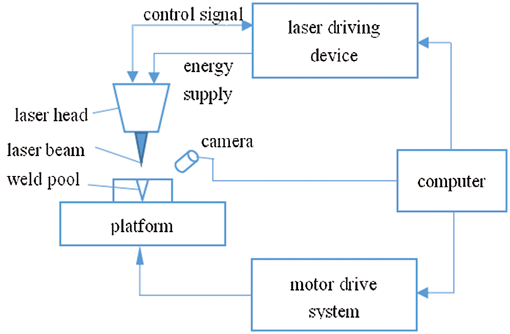
Figure 1: Schematic of the laser welding control system

3  Nonlinear System Identification of Welding Process Based on RBF Neural Networks

The radial basis function (RBF) neural network is a class of artificial neural networks with good nonlinear approximation ability and global optimization capability. Further, it can handle difficult analytical solutions in complex systems, so it has good potential for generalization. The typical RBF network structure comprises a three-layer feed-forward network (with an input layer, hidden layer, and output layer), wherein the activation function of the hidden layer is the RBF, which can easily transform the input variable into the output variable [19–24]. The input layer can cause nonlinear changes in the hidden layer, which are then transferred to the output layer, with each layer having connecting weight variables. This allows the network to be trained rapidly, avoiding the local optimum, and achieving a good nonlinear approximation.

3.1 Basic Hypothesis

The description of the nonlinear SISO system utilizes the nonlinear extended auto-regressive moving average model (NARMAX).

y(k)=f(y(k−1),...,y(k−ny);u(k−d),...,u(k−nu)) (1)

In Eq. (1), u(.) indicates the input of the model, y(.) represents the output of the system, f(.) shows the nonlinear relationship between the input and the output. The pure delay of the system is d, which usually takes the value d ≥ 1.

To establish the above-mentioned nonlinear system model, an RBF neural network was selected to apply the NARMAX model, namely

ym(k)=fm(y(k−1),...,y(k−ny);u(k−d),...,u(k−nu)) (2)

The structure of the RBF neural network system based on the nonlinear SISO system is shown in Fig. 2.

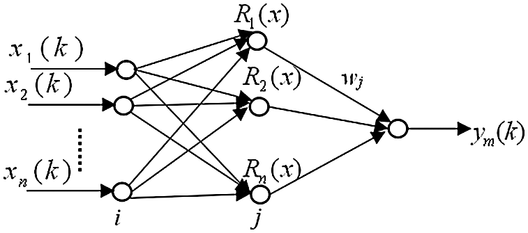
Figure 2: RBF neural network structure

In Fig. 2, the RBF neural network is Rj(x), j = 1,2,…, m.

It is assumed that the system can be represented by the following relations:

x=[x1(k),x2(k),...,xn(k)]T=[y(k−1),...,y(k−ny);u(k−d),...,u(k−nu)]T (3)

where n represents the number of input layer nodes, n = ny+nu-d+1; ym(k) represents the system output. The high-Gaussian function is the activating function of the hidden layer in the RBF neural network system.

Rj(x)=exp⁡(−‖x−cj‖22bj2), j=1,2,...,m (4)

In Eq. (4), cj is the jth activation function centre of the hidden layer, cj=[cj1,cj2,...,cjn]T ; bj determines the width deviation of the centre-point function, which can be freely selected within a limited range; and m is the node number of the hidden layer of the system.

The derivative of the basic function is given:

∂Rj(x)∂bj=Rj(x)‖x−cj‖22bj3 (5)

∂Rj(x)∂cji=Rj(x)(xi−cji)bj2 (6)

3.2 Output Calculation of RBF Network

The output of the neurons of the hidden layer can be derived from x(k)=[x1(k),x2(k),...,xn(k)]T and Eq. (3):

Rj(x(k))=exp⁡(−‖x(k)−cj(k−1)‖2bj2(k−1)), j=1,2,...,m (7)

Thus, the system output can be obtained based on the RBF neural network structure and the above analysis:

e(k)=y(k)−ym(k) (8)

wj(k−1) denotes the neuronal connection weights between the j th hidden layer and the j th output layer in Eq. (7), when the system is at k−1 time.

The error of the training RBF network can be represented as

e(k)=y(k)−ym(k) (9)

where y(k) is the desired actual output of the neural network and ym(k) is the ideal output of the system model.

The index function of the system is

E(k)=12e2(k) (10)

3.3 Adjustment of the Connection Weights of the RBF Network Layers based on the Learning Algorithm

The detailed derivation of the weight learning algorithm is based on the gradient-descent method, and is shown in previous studies [25–27].

Combining Eqs. (8) and (9), the connection weights between the hidden layer and the output layer of the RBF system can be obtained as follows:

δ(2)=∂E(k)∂ym(k)=∂E(k)∂e(k)∂e(k)∂ym(k)=−e(k) (11)

Modifying Eqs. (8) and (11), we can obtain the following formula:

∂E(k)∂wj(k−1)=∂E(k)∂ym(k)∂ym(k)∂wj(k−1)=δ(2)Rj(x(k))=−e(k)Rj(x(k)) (12)

The weight-learning algorithm between the hidden layer and the output layer can be represented by

Δwj(k−1)=−η∂E(k)∂wj(k−1)=ηe(k)Rj(x(k)) (13)

wj(k)=wj(k−1)+Δwj(k)+α(wj(k−1)−wj(k−2)) (14)

where η is the learning ratio and α is the inertia factor.

Combining Eqs. (7) and (10), the learning algorithm of the parameters bj(k) and cji(k) in the hidden-layer Gaussian function can be derived as follows:

δ(1)=∂E(k)∂Rj(x(k))=∂E(k)∂ym(k)∂ym(k)∂Rj(x(k))=δ(2)wj(k−1) (15)

On the basis of Eqs. (4), (5), and (14), the following can be derived:

∂E(k)∂bj(k−1)=∂E(k)∂Rj(x(k))∂Rj(x(k))∂bj(k−1)=−e(k)wj(k−1)Rj(x(k))‖x(k)−cj(k−1)‖2bj3(k−1) (16)

∂E(k)∂cji(k−1)=∂E(k)∂Rj(x(k))∂Rj(x(k))∂cji(k−1)=−e(k)wj(k−1)Rj(x(k))x(k)−cj(k−1)bj2(k−1) (17)

Then, the learning algorithms of bj(k) and cji(k) are

Δbj(k)=−η∂E(k)∂bj(k−1)=ηe(k)wj(k−1)Rj(x(k))‖x(k)−cj(k−1)‖2bj3(k−1) (18)

bj(k)=bj(k−1)+Δbj(k)+α(bj(k−1)−bj(k−2)) (19)

Δcji(k)=−η∂E(k)∂cji(k−1)=ηe(k)wj(k−1)Rj(x(k))x(k)−cj(k−1)bj2(k−1) (20)

cji(k)=cji(k−1)+Δcji(k)+α(cji(k−1)−cji(k−2)) (21)

3.4 Simulation

Here, a nonlinear model is designed that considers the various factors relevant to the welding process. u represents the welding speed of the neural network input and y is the weld width of the neural network output [27–29].

y(k)=u3(k−2)+u4(k−3)+0.8+y2(k−1)1+y2(k−1)+y3(k−2) (22)

The input signal is u(k)=0.8sin⁡(0.01πk) and the input is {y(k−1),y(k−2);u(k−2),u(k−3)} , the output is ym(k) , the learning ratio is η=0.5 , and the inertia factor is α=0.05 . The fitting process of the network output and the actual output in the RBF neural system are shown in Figs. 3–7.

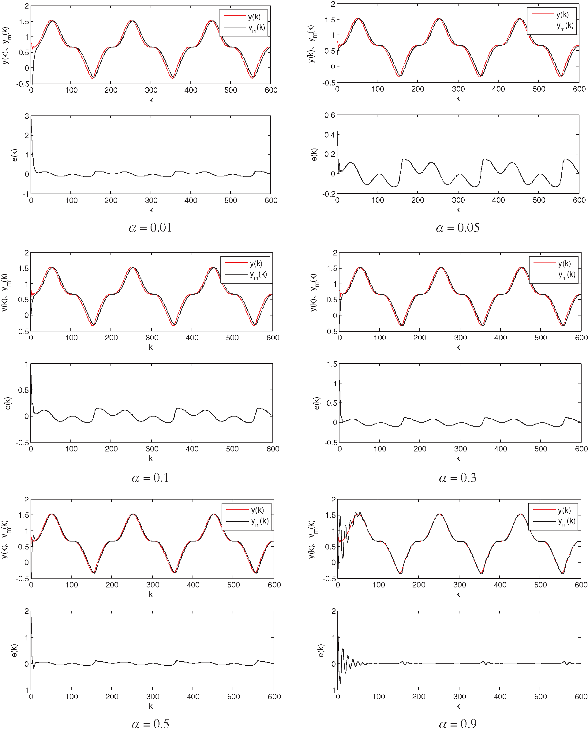
Figure 3: Recognition results for the RBF neural network ( η=0.1 )

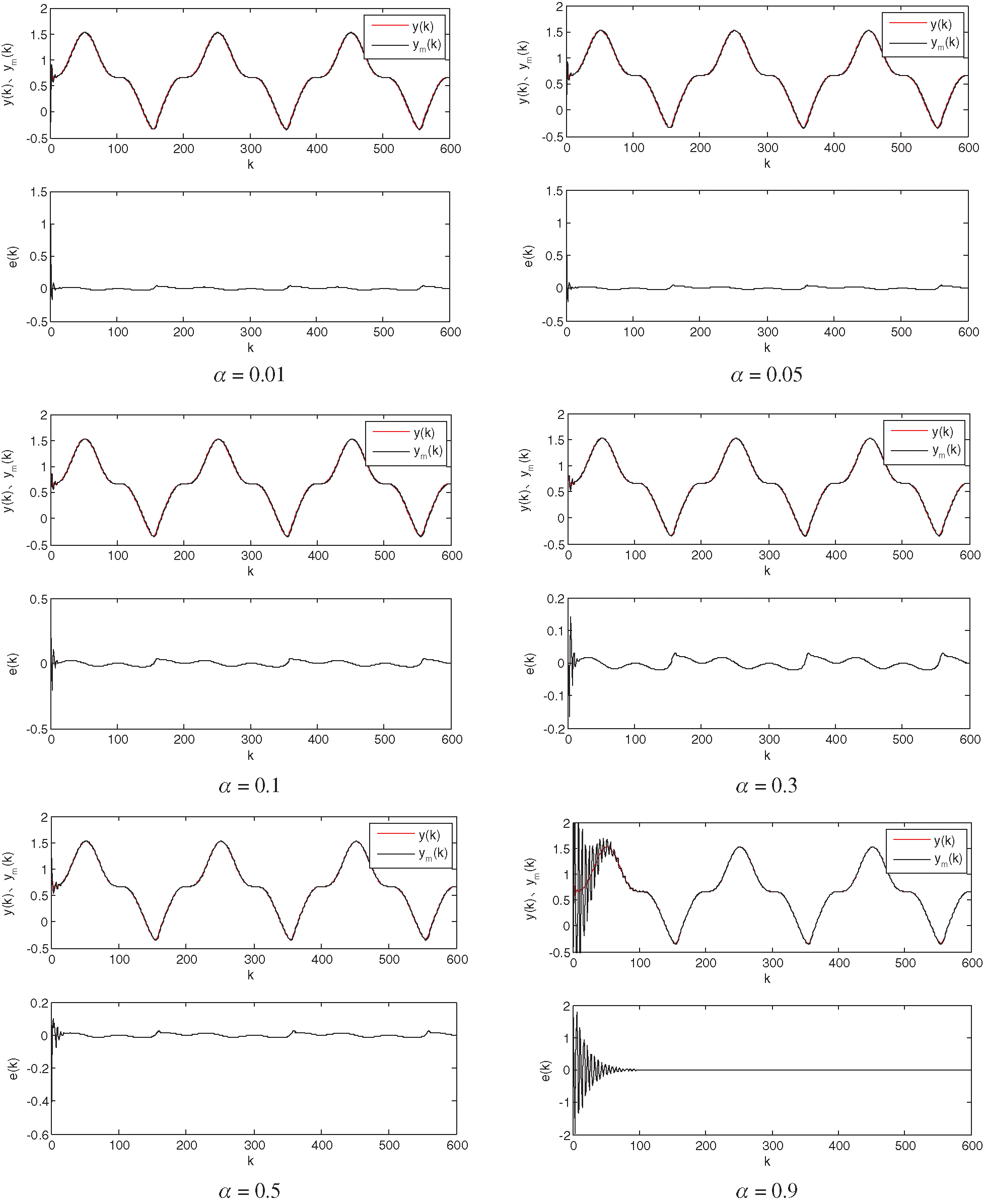
Figure 4: Recognition results for the RBF neural network ( η=0.5 )

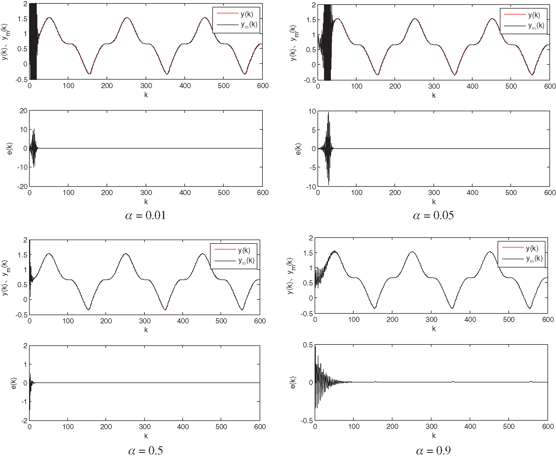
Figure 5: Recognition results for the RBF neural network ( η=1 )

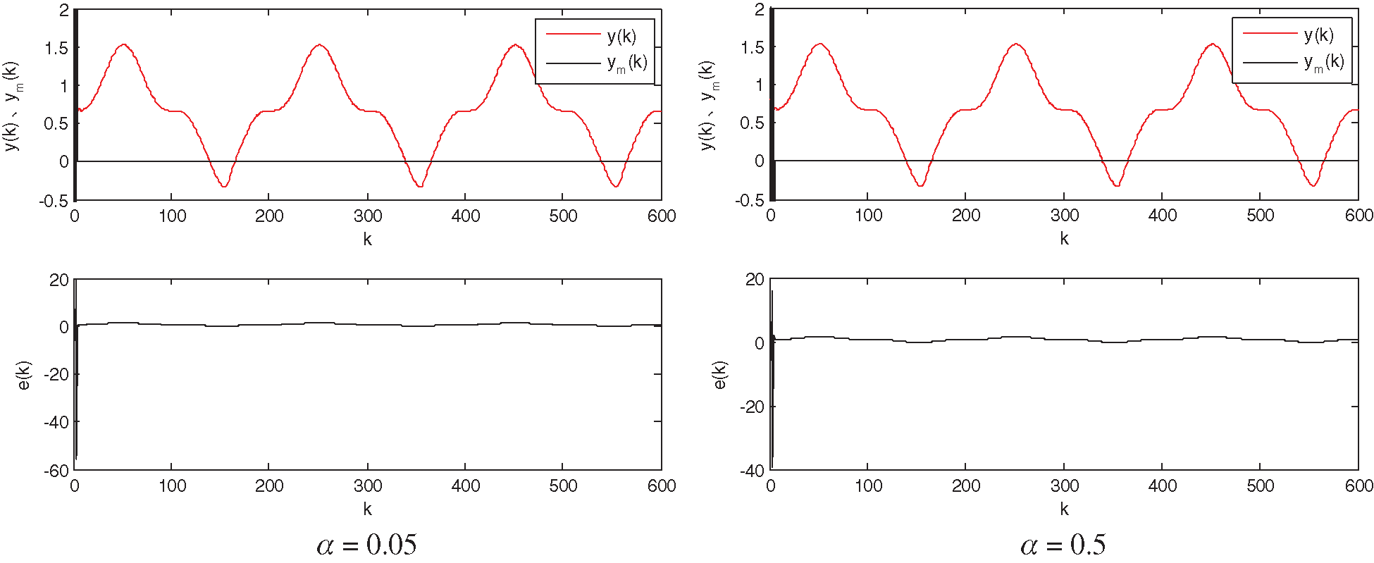
Figure 6: Recognition results for the RBF neural network ( η=2 )

It can be seen from Figs. 3–6 that the learning ratio η and the inertia factor α have an important influence on the training of the RBF neural network. If η and α are too small, the convergence speed of the system will reduce, the training process will become longer, and errors will increase, resulting in low identification accuracy. If η and α are too large, the network convergence speed will increase, the training time is shorter, and the training process will oscillate and diverge. Therefore, optimum values for the learning ratio η and inertia factor α exist, which can provide both good identification speed and accuracy for the training model. Through experimentation, we select the learning ratio η=0.5 and the inertia factor α=0.05 .

As can be seen in Fig. 7, when the learning ratio and the inertia factor are determined, changing the node number of the hidden layer will have a greater impact on the network. When the number of hidden-layer nodes is small, the desired output and actual output will not be well fitted; when the number of hidden-layer nodes is large, the training process will be prone to oscillation and does not achieve good identification results. Therefore, we choose a 4–6–1 structure for the RBF neural network.

Through the above analysis, when identifying the system based on the RBF neural network, the network parameters of the learning ratio η , inertia factor α , initial bj(0) and cji(0) values of the Gaussian basis functions, initial value wj(0) of the weights, and hidden-layer nodes m will have different degrees of impact on the network’s training processes.

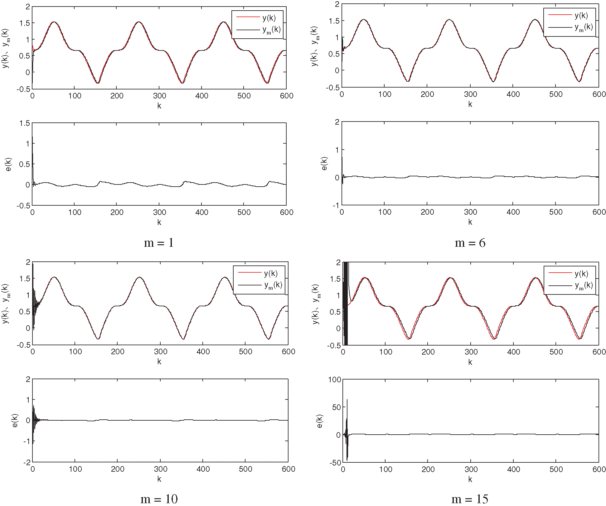
Figure 7: Recognition results for the RBF neural network ( η=0.5 , α=0.05 )

4  Application of RBF Neural Network PID Self-Tuning Control to Laser Welding Control

The structure of the self-tuning PID control based on RBF neural networks is shown in Fig. 8.

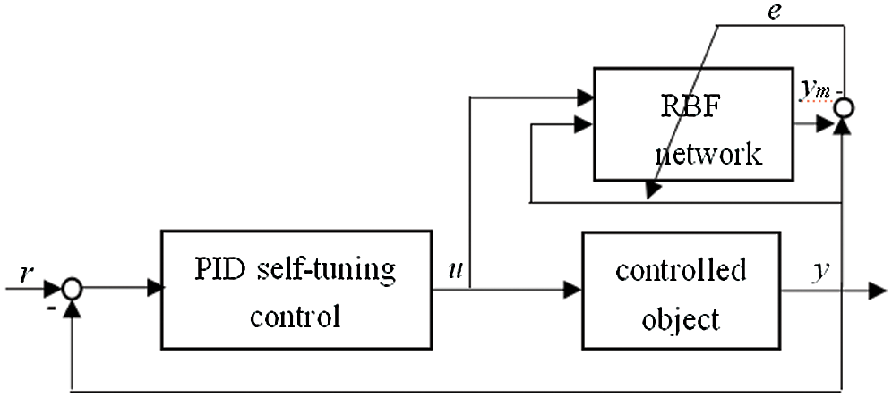
Figure 8: Structure of the self-tuning PID control-based method on the RBF neural network

The incremental PID control algorithm is used in this system. If ec(k)=r(k)−y(k) , the following relations can be obtained:

Δu(k)=Kp(k−1)[ec(k)−ec(k−1)]+Ki(k−1)e(k)+Kd(k−1)[ec(k)−2ec(k−1)+ec(k−2)] (23)

where Kp , Ki , and Kd are PID tuning parameters,

{xc1(k)=ec(k)−ec(k−1)xc2(k)=ec(k)xc3(k)=ec(k)−2ec(k−1)+ec(k−2) (24)

Therefore, the control law is

u(k)=u(k−1)+Δu(k) (25)

and the index function is

Ec(k)=12ec2(k) (26)

By adjusting the PID parameters using the gradient-descent method, the following results can be obtained:

{ΔKp(k)=−ηc∂Ec(k)∂Kp(k−1)=−ηc∂Ec(k)∂y(k)∂u(k)∂y(k)∂u(k)∂Kp(k−1)=ηcec(k)∂y(k)∂u(k)[ec(k)−ec(k−1)]ΔKi(k)=−ηc∂Ec(k)∂Ki(k−1)=−ηc∂Ec(k)∂y(k)∂u(k)∂y(k)∂u(k)∂Ki(k−1)=ηcec(k)∂y(k)∂u(k)ec(k)ΔKd(k)=−ηc∂Ec(k)∂Kd(k−1)=−ηc∂Ec(k)∂y(k)∂u(k)∂y(k)∂u(k)∂Kd(k−1)=ηcec(k)∂y(k)∂u(k)[ec(k)−2ec(k−1)+ec(k−2)] (27)

The learning algorithm of the PID parameters is as follows:

{Kp(k)=Kp(k−1)+ΔKp(k)+αc(Kp(k−1)−Kp(k−2))Ki(k)=Ki(k−1)+ΔKi(k)+αc(Ki(k−1)−Ki(k−2))Kd(k)=Kd(k−1)+ΔKd(k)+αc(Kd(k−1)−Kd(k−2)) (28)

When calculating the PID parameters using Eqs. (27) and (28), we need information regarding the Jacobian ∂y(k)∂u(k) . However, as the controlled object model is unknown and the Jacobian information cannot be obtained directly, the following approximation is made:

∂y(k)∂u(k)≈∂ym(k)∂u(k) (29)

The RBF network input is represented by

x=[x1(k),x2(k),...,xn(k)]T=[y(k−1),...,y(k−ny);u(k−d),...,u(k−nu)]T (30)

Therefore, xny+1(k+1)=u(k) , and the following result can be obtained by combining Eqs. (7) and (8):

∂ym(k)∂u(k)=∑j=1m∂Rj(x(k))∂u(k)=∑j=1mwj(k−1)Rj(x(k))cj(ny+1)(k−1)−u(k)bj2(k−1) (31)

If the ny , nu , and d values of the nonlinear structural system are known, the steps for self-tuning PID identification and control based on the RBF neural network will be as follows:

(1) Input the initial data of the system, and set the initial parameters bj(0) , cji(0) , and wj(0) of the RBF network and system-related parameters of the hidden layer neuron number m , the learning ratio η , and the inertia factor α . Set the initial value of the PID parameters Kp(0) , Ki(0) , and Kd(0) , along with the training parameters of the learning ratio ηc and inertia factor αc .

(2) Sample the actual system output y(k) and the reference input yr(k) , and calculate u(k) using Eqs. (22)–(24).

(3) Calculate the system output ym(k) using Eqs. (7) and (8). The Jacobian information can be derived using Eq. (29) and (30).

(4) Use Eqs. (26) and (27) to calculate the PID parameters Kp(k) , Ki(k) , and Kd(k) .

(5) Use Eqs. (13), (18), and (20) to compute the network parameters wj(k) , bj(k) , and cji(k) , respectively.

(6) Return to Step (2) and continue the loop.

If the welding speed u is the system input, and the weld width y is the system output [29,30]; therefore, the nonlinear system of the laser welding control follows the given relation:

y(k)=u3(k−2)+u4(k−3)+0.8+y2(k−1)1+y2(k−1)+y3(k−2) (32)

The input signal is a square wave signal yr(k)=0.25sign(sin⁡(0.002πk))+0.75 , the structure of the RBF neural network is 6–10–1, the input is {y(k−1),y(k−2);u(k),u(k−1),u(k−2),u(k−3)} , and the output is ym(k) . The network learning ratio is η=0.5 and the inertia factor is α=0.05 . Assuming that the PID parameters’ initial values are 0, the PID parameter of the learning ratio is ηc=1 and that of the inertia factor is αc=0.1 .

With changes in the data length L, various indicators will change in different ways if the structural parameters remain unchanged. If L < 3500, the control results and network fitting results are improved, the Jacobian information is relatively stable, and the PID parameters change with periodic variations in the data length L. When L ≥ 3500, the entire system begins to oscillate and diverge; if the system based on the RBF network does not adjust the stable PID parameters, the proportional parameters and integral parameters will continue to increase, all of which will exacerbate the system divergence.

If the learning ratio ηc and the inertia factor αc of the PID parameters are adjusted at this time, the system results will become stable, as shown in Fig. 9. However, the proportional parameters and integral parameters still continue to increase, affecting the stability and measurement accuracy of the system.

If the various parameters are set to reasonable values, the results will be accurate. The results regarding system identification based on the RBF neural network and self-tuning PID control based on the RBF neural network perform well.

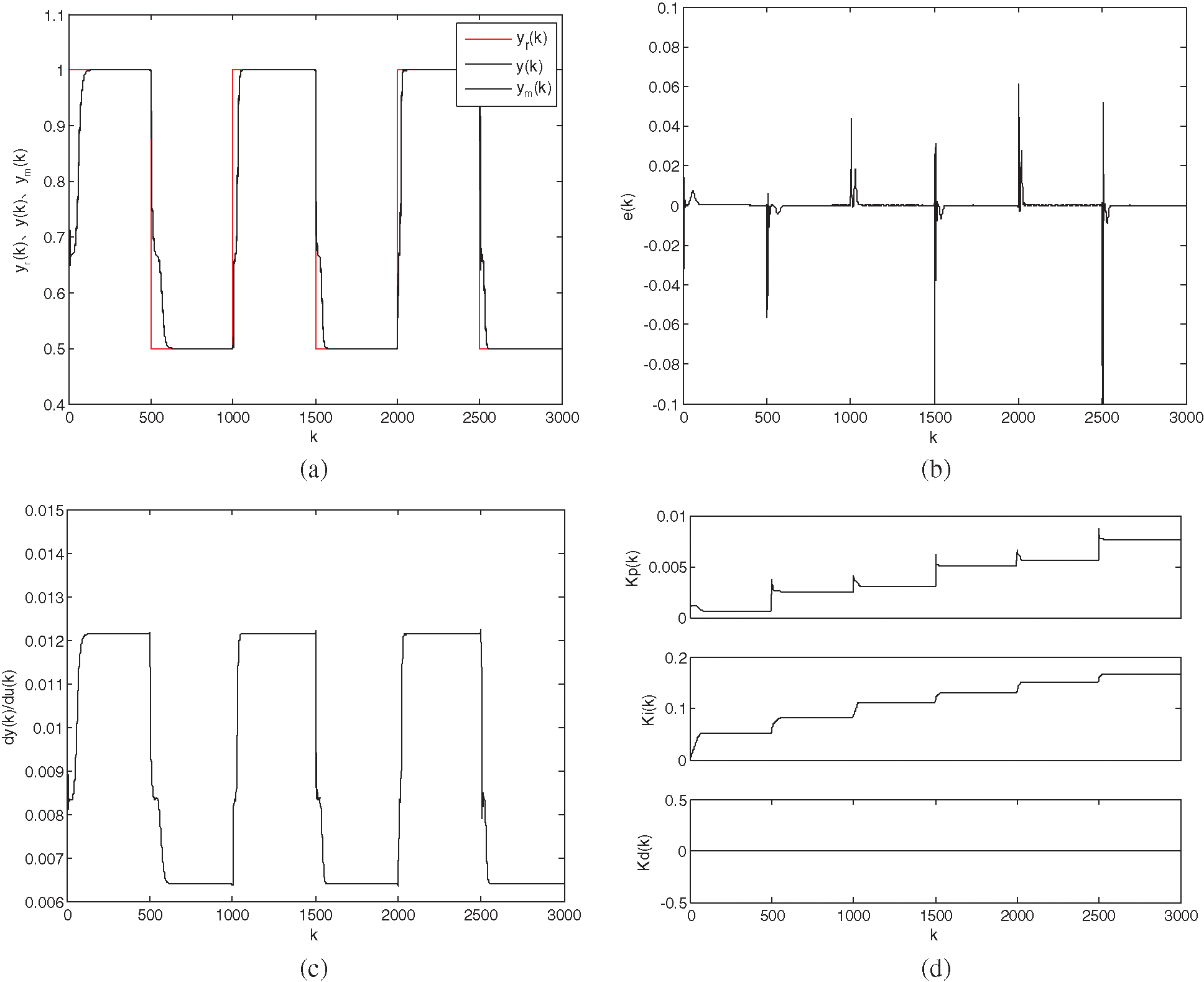
Figure 9: Variations in the plots with the learning ratio ηc and the inertia factor αc of PID parameters when the system diverges ( η=1 , α=0.1 ) (a) Control results and network-fitting result curves (b) Fitting-error curves (c) Jacobian-information curves (d) Adaptive-adjustment curves of PID parameters

5  Conclusion

In this study, self-tuning PID control based on the RBF neural network is used to identify and control a nonlinear laser welding system with unknown parameters. The simulation results show that the control algorithm has high identification accuracy, and is practical and effective. The weld width quickly reached expected values, the system remains stable and robust. We expect the results of this study to provide relevant information for the establishment of a new, smart green welding manufacturing protocol for modern equipment.

The laser welding control technology investigated in this study can improve the applicability of laser technology, and can greatly improve the efficiency and accuracy of welding. Furthermore, it is advantageous in terms of its high power density and fast energy release, improving operation efficiency. The focus of laser technology is smaller, making the adhesion between welded materials better without causing much damage and material deformation. These systems can meet the welding requirements of different materials—both metals and non-metals—and because of the penetration and refractivity of the laser itself, an arbitrary focus within 360° can be realized according to the trajectory of the light itself.

Acknowledgement: I would like to thank the members of my team for their hard work, the University for its equipment and research space, and the government for its ample funding.

Funding Statement: This work was supported by the Youth Backbone Teacher’s training program for Henan colleges and universities under Grant No. 2016ggjs-287; the Science and Technology Project of Henan province, under Grant Nos. 172102210124 and 202102210269; and the Key Scientific Research Projects in Colleges and Universities in Henan, Grant No. 18B460003.

Conflicts of Interest: The authors declare that they have no conflicts of interest to report regarding the present study.

This work is licensed under a Creative Commons Attribution 4.0 International License, which permits unrestricted use, distribution, and reproduction in any medium, provided the original work is properly cited.